Constraint-based Pattern Mining in Multi-Relational Databases
Siegfried Nijssen∗ ∗Departement Computerwetenschappen
Katholieke Universiteit Leuven Celestijnenlaan 200A, 3000 Leuven, Belgium
A´ıda Jim´enez† Tias Guns∗
†Department of Computer Science and Articial Intelligence ETSIIT–University of Granada
18071 Granada, Spain
Abstract—We propose a new framework for constraint-based pattern mining in multi-relational databases. Distinguishing features of the framework are that (1) it allows finding patterns not only under anti-monotonic constraints, but also under monotonic constraints and closedness constraints, among oth-ers, expressed over complex aggregates over multiple relations; (2) it builds on a declarative graphical representation of constraints that links closely to data models of multi-relational databases and constraint networks in constraint programming; (3) it maps multi-relational pattern mining tasks into constraint programs. Our framework builds on a unifying perspective of multi-relational pattern mining, relational database tech-nology and constraint networks in constraint programming. We demonstrate our framework on IMDB and Finance multi-relational databases.
Keywords-pattern mining; multi-relational databases I. INTRODUCTION
Traditional itemset mining is a popular pattern mining task in the field of data mining. It consists of finding sets of items that occur frequently together in a binary database [1]. The binary database typically consists of one binary relation relating items to transactions. In several publications it has already been observed that this single-relational setting is too limiting when dealing with multi-relational databases [2], [3], [4], [5]: in multi-relational databases one typically finds multiple relations, of which the transformation into one relation can be hard or undesirable. Hence, specialized algorithms were developed that operate on multi-relational data directly.
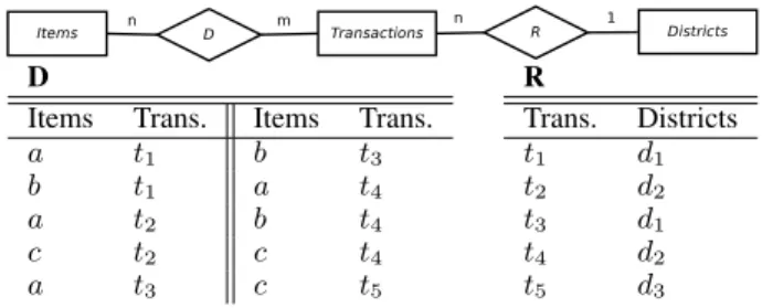
Consider a multi-relational database in the financial do-main, in which items describe transactions and transactions belong to a district. Figure 1 describes the entity-relationship diagram and provides an example instance of this diagram.
Most algorithms for multi-relational pattern mining fo-cus on finding frequent patterns expressed as conjunctive queries. A conjunctive query is a conjunctive first-order logic formula with only existential quantifiers. An example pattern, in conjunctive query form, for the above data is:
∃Y :R(X, Y)∧D(Y, a)∧D(Y, b). (1) This formula can be satisfied by districts (variableX) having a transaction (variableY) that has both itemsaandb. In our †This research was performed while visiting the DTAI group in Leuven.
D
Items Trans. Items Trans.
a t1 b t3 b t1 a t4 a t2 b t4 c t2 c t4 a t3 c t5 R Trans. Districts t1 d1 t2 d2 t3 d1 t4 d2 t5 d3
Figure 1: Running example of a relational database
example, districts d1 andd2 would satisfy the formula. In these conjunctive query mining algorithms, thefrequencyor support of the query is determined by the number of districts X for which the formula is true. In the example above, the support would be 2. The typical task is to find all conjunctive queries that are frequent, i.e. queries for which the support exceeds a predefined threshold.
A task that has received considerably less attention is that of finding multi-relational patterns adhering to more com-plex constraints. Imposing additional constraints in multi-relational pattern mining could be useful in many appli-cations. Consider our financial example again. In the con-junctive query mining setting, a district is already counted in the support of the example query even if it has only one transaction containing both items a and b. If one is looking for patterns that clarify common behavior accross a large number of districts, this pattern is not very useful. Instead, one should be able to impose that a certain number of transactions (more than one) within a district should contain the set of items. Similarly, one could wish to define constraints on otheraggregates, such as the maximum number of transactions of a certain kind, or on the average value of transactions in a number of districts.
In this paper we propose an approach for formalizing a number of constraint-based multi-relational pattern mining problems that have not yet been addressed by any other system. In addition to aggregation and complex counting constraints expressed over multiple relations, it also supports expressingcondensed representationsconstraints. Typically, a very large number of patterns is found when only a minimum support constraint is employed. Condensed
repre-sentations can help in overcoming this problem by restricting the search to non-redundant patterns. Examples in the single-relation case areclosedormaximalpatterns [6]. Again, these condensed representations have not received much attention in the multi-relational pattern mining literature.
The distinguishing feature of our approach is that it treats multi-relational pattern mining as a constraint satisfaction problem. This extends the work of [6] that addresses tradi-tional constraint-based mining in a single-relatradi-tional setting. Studying pattern mining as a constraint satisfaction problem has several advantages. The most important is that the approach is general and does not require the implementation of new solver algorithms. We can exploit existing solver technology and the efficient search algorithms they provide. We can build on concepts and principles that have been stud-ied for many years in the artificial intelligence community already, but for which the applicability in multi-relational data mining has not been recognized yet.
A feature that is of particular interest in our framework is that it allows for declarative data mining by means of visual primitives. The visual representation makes the link to the underlying database model explicit, while it also clarifies the link with constraint networks in the constraint satisfaction literature [7].
The paper is organized as follows. We start with a more detailed discussion of the literature on multi-relational pattern mining. In Section III we give a high level overview of our approach for modeling multi-relational pattern mining problems. Section IV illustrates it on several examples. Section V shows how the high level modeling primitives can be transformed into low-level database and constraint programming primitives. After demonstrating the capabili-ties in a number of experiments we conclude.
II. RELATEDWORK
Many algorithms for finding frequent conjunctive queries in multi-relational databases exist [2], [3], [4], [8]. An advantage of the frequent conjunctive query mining task is that search procedures can exploit the anti-monotonicity property of the minimum support constraint. Essentially, search can proceed from general to specific queries, where specialization takes place by adding literals. The query of equation (1) is for instance a specialization of this query:
∃Y :R(X, Y)∧D(Y, a) (2) If the support of this more general query is too low, then more specific queries such as the one in equation (1) can not be frequent either. In this way, the anti-monotonicity property can be used to prune large parts of the search space. The addition of aggregation constraints to the mining pro-cess was previously studied by Knobbe et al. [5]. Building on a visual representation of patterns as selection graphs, aggregates were added to patterns. In our running example
the following is a selection graph which only selects districts with multiple transactions related to both itemaandb:
Note that a selection graph is a representation of a pattern. The free variable, used to define support, is indicated by a black node. Nodes correspond to entities while edges repre-sent relationships that need to be prerepre-sent between objects in the entities. If one would represent the data as graphs too, the discovery of multi-relational patterns could be seen as a type of graph or tree mining [9], with the distinguishing feature that edges in the pattern can be labeled with aggregates; however, current graph and tree mining algorithms do not currently support the constraints we considered in this paper. A problem of the approach of Knobbe et al. is that it is limited by its enumeration of selection graphs by adding nodes in the graph. For instance, the following extension of a selection graph would lead to a selection graph with highersupport:
To deal with this, Knobbe et al. do not allow extensions that lead to generalizations instead of specializations. As a result, this method is incapable of discovering certain patterns, such as the patterns in the figure above. To find such patterns, a fundamentally different search procedure is needed.
Additionally, the approach of Knobbe et al. focuses on aggregates and is not capable of finding closed or maximal patterns in multi-relational databases. Closed and maximal patterns are often used as condensed representations, but have rarely been studied in the context of multi-relational databases [10].
In this paper, we propose an approach that is comple-mentary to these earlier approaches. Instead of focusing on the enumeration of conjunctive queries or selection graphs under a support constraint, we propose an approach in which the structure of the patterns is more rigid, but in which a richer class of constraints can be imposed. In our approach the user fixes the variables in the mining task in advance, and defines constraints on these variables. Having a fixed set of variables allows for different search procedures, and hence for solving tasks which are not supported by current conjunctive query mining systems.
We are aware of several earlier approaches that also take a constraint satisfaction approach to multi-relational pattern mining: in the framework of compositional data mining (CDM) [11] traditional mining algorithms are run on
separate tables; the individual results are then post-processed into solutions over multiple relations. Clearly, this approach is only feasible in case sufficient constraints can be imposed on the tables individually. Mining chains of relations over 2 relations has been studied as well [12]. Algorithms for finding patterns in tensors [13] focus on data with a single table of high arity, while our work focuses on a setting with multiple tables.
Our approach is building on the constraint programming for itemset mining framework [6]. Constraint programming provides a general methodology for solving constraint satis-faction problems (CSP) [7]. By using the CP methodology, it was already found in [6] that it is possible to perform an effective pattern search when constraints are not anti-monotonic, in single relational databases. In this paper we extend that approach to the multi-relational setting.
III. MODELINGMULTI-RELATIONALPATTERNMINING The main idea behind our approach is to model multi-relational pattern mining tasks as constraint satisfaction problems, by means of a high-level modeling language. In this section we discuss this modeling language formally, including the high-level primitives that are used to model multi-relational pattern mining tasks. We will visualize these primitives subsequently.
We assume given a multi-relational database consisting of a number of entities E = {E1, . . . , En}, and a set of relations R={R1, . . . , Rm}. Each entity consists of a set of objects, i.e.Ei={o1, o2, . . . , oℓ}, which can be thought of as tuples in the entity. For reasons of simplicity, we here assume that relations are binary and relate two entities e1(Ri)ande2(Ri), i.e. Ri⊆e1(Ri)×e2(Ri).
We model the multi-relational pattern mining task on this database by means of a fixed set of variables and a set of constraints between the variables. Each assignment to these variables that satisfies all constraints reflects one pattern that is found by the algorithm. The model can contain one or more variables for each entity; the entity to which a variable belongs is identified by e(V). The domain of a variableV consists of asetof objects, i.e.D(V) = 2Ee(V). For each set variable V the task is to find a subset of objects of Ee(V) that satisfies all given constraints.
The basic constraints that we consider in this paper are: Object Constraints: An object constraint is expressed byobject(V, p), wherepis a predicate that can be evaluated on each object ine(V)individually. It is satisfied when
object(V, p)⇔(∀o∈V :p(o)).
Object constraints allow to filter and select certain objects of an entity.
Size Constraints: A size constraint is expressed by
minsize(V, θ) or maxsize(V, θ), where θ is a threshold. Constraint minsize(V, θ)is defined by:
minsize(V, θ)⇔(|V| ≥θ).
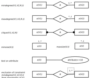
Figure 2: Visualization of constraints
Degree Constraints: A degree constraint on a relation R is expressed by mindegree1(V1, V2, R, θ),
maxdegree1(V1, V2, R, θ), mindegree2(V1, V2, R, θ) or
maxdegree2(V1, V2, R, θ). mindegree1(V1, V2, R, θ) constrains every element of V1 to be related to at least θ elements inV2 through R and is defined by:
mindegree1(V1, V2, R, θ)⇔
(∀o1∈V1:|{o2∈V2|(o1, o2)∈R}| ≥θ), where it is assumed thate(V1) =e1(R)ande(V2) =e2(R). Other constraints are defined similarly.
Biclique Constraints: A biclique constraint on a rela-tionR is expressed bybiclique(V1, V2, R)and defined by
biclique(V1, V2, R)⇔(∀o1∈V1, o2∈V2: (o1, o2)∈R). The problem that we study is to findallassignments to all set variables such that all constraints in a set of constraints C={C1, . . . , Cs} are satisfied.
A useful feature of our primitives is that we can visualize them in diagrams which are similar to entity-relationship di-agrams. The mapping of basic constraints to visual building blocks is given in Figure 2. Even though similar to entity-relationship diagrams, these building blocks do not represent properties of the data model, but constraints that patterns should fulfill. In contrast to selection graphs and conjunctive queries the nodes do not represent logical variables in a pattern set variables in a CSP. The constraint visualisation is close toconstraint networksin CP: every entity represents a variable, while every relation defines a constraint. Maximality.Without further restrictions, there can be many solutions to problems specified by the above constraints. For instance, any subset of objects that are part of a biclique, also constitute a biclique. This results in large numbers of syntac-tically less interesting patterns. To avoid such patterns, we introducemaximality constraintson set variables. Intuitively, a set variable has a maximal value if it is impossible to
Figure 3: Visualizations of Itemset Mining
add an object to it, without violating at least one constraint. To provide the user with modeling freedom, the user can specify for every variableV the constraints with respect to which it needs to be maximal, i.e. a set maxC(V) ⊆ C. Every constraint in maxC(V) should involve the variable V. A constraint only involves a variable if a situation can exist in which adding an object to the variable falsifies a satisfied constraint (keeping other variables unmodified). For instance, the constraint mindegree1(V1, V2, R, θ) does not involve variableV2, as adding an object toV2 will increase the degree and can thus never have a negative effect on the satisfaction of the constraint.
Hence, a solution satisfies the maximality constraints for a variableV iff for allo∈e(V)\V, if we add oto V, but keep all other variables unmodified, the conjunction of all constraints inmaxC(V)is no longer satisfied.
In our visualisation we assume maximality with respect to all involved constraints by default. Constraints that are excludedare marked by a dashed line.
Overall, a model in our language is specified by a tuple hE,R,V,C,maxC, ei, with: a set of entities E; a set of relations R, each linking two entities; a set of variables V; a mapping from variables to entities e; a set of basic constraints C; a set of maximality constraints for each variableV.
Given a (multi-)relational database, and its corresponding ER diagram, the intended methodology is that the user spec-ifies a model using the primitives specified in this section. The system subsequently discovers all patterns satisfying the constraints on the multi-relational database. We will now first illustrate this approach on several example instances; subsequently, we will discuss how solutions are calculated.
IV. EXAMPLE INSTANCES
The visualizations of our examples are given in Figure 3 and Figure 4; the first three settings model single-relational mining settings and are based on [6].
Frequent Itemset Mining: Our first example is tra-ditional frequent itemset mining (Figure 3(a)). Let I =
{1, . . . , m} be a set of items, and T = {1, . . . , n} a set
of transactions. An itemset database Dcan be seen as a set of tuples in I × T. The traditional formalization is to find all sets for which freq(I, D)≥ minsup, where freq(I, D)
is defined as follows:
freq(I, D) =|{t∈ T |∀i∈I: (t, i)∈D}|.
Assuming two entities, items and transactions, and set variables I andT over these entities, we can now express this problem in our framework as:
minsize(T,minsup)∧biclique(I, T, D), withmaxC(T) ={biclique(I, T, D)}. Or, equivalently:
mindegree1(I, T, D,minsup)∧biclique(I, T, D), withmaxC(T) ={biclique(I, T, D)}.
Closed Frequent Itemset Mining: Closed itemsets are a popular condensed representation for the set of all frequent itemsets and their frequencies. Closed itemset mining is similar to frequent itemset mining except that also the itemset is required to be maximal with respect to the set of transactions. This is enforced by choosing as maxi-mality constraints: maxC(T) = {biclique(I, T, D)} and
maxC(I) ={biclique(I, T, D)} (Figure 3(b)).
Maximal Frequent Itemset Mining: Maximal frequent itemsets are another condensed representation for the set of frequent itemsets, in which it is required that any superset of a frequent itemset is infrequent. This is enforced by changing the maximality constraints as follows:
maxC(T) = {biclique(I, T, D)} and maxC(I) =
{mindegree1(I, T, D,minsup),biclique(I, T, D)}
(Figure 3(c)). The net effect is that if items can be added without violating the degree or other maximality constraints, then this must be done.
Multi-Relational Itemset Mining: This setting (Fig-ure 3(d)) reflects a simplified version of the running example of the introduction, consisting of 2 relations, representing relationships between items and transactions and between transactions and districts. The crucial element in it is that selected districts are required to have a number of trans-actions mintran > 1, each of which containing all items selected in Items.
In the example database of the introduction a solu-tion is for instance Items = {a, b};Transactions =
{t1, t3, t4};Districts = {d1, d2}. Note that in contrast to conjunctive queries, which only list items, solutions in our setting also contain sets of transactions and districts. The apriori defined constraints express the relationships between these objects.
Closed Multi-Relational Itemset Mining: Closed pat-tern mining in multi-relational databases is a problem which has been studied rarely [10]. We can straightforwardly re-strict the search to closed patterns in the running example by enforcing maximality with respect to the items (Figure 3(e)).
Figure 4: Visualizations of Discriminative Itemset Mining
Static Discriminative Itemset Mining: This setting re-flects a more traditional approach to discriminative pattern mining, in which essentially we partition the transactions in positive and negative examples and we are interested in find-ing itemsets distfind-inguishfind-ing these two classes of transactions. Figure 4(a) provides the model.
Note that we could evaluate this query in two steps: we could first use traditional database queries to generate a dataset with positive and negative examples; subsequently, we could perform pattern mining on this data. However, from a declarative perspective, we can formalize the entire task in one language; the solver will have the task to find an effective way of evaluating this query.
Dynamic Discriminative Itemset Mining: Whereas in the previous setting the classes were defined in advance, a more dynamic setting can also be formalized. Assume that for each pair of districts we have a relation encoding which districts are considered to be close to each other. Then we could be looking for a pair of districts, which, even though close to each other, can be distinguished from each other based on the descriptors of transactions. The model is given in Figure 4(b).
V. EVALUATIONSTRATEGY
Our strategy for finding patterns for a given high-level model consists of two steps. In the the first step, all the necessary information for the CSP is collected from the database. Ideally, many constraints will already be factored out using the database management system, as this would reduce the size of the CSP that will be solved in the second stage. In the second step, an existing constraint satisfaction solver is used to find patterns. Before doing this, we transform the high-level modeling primitives to low-level primitives provided by the CP system.
A. Step 1: Pre-Processing
The aim of this step is the extraction of the necessary variable domains and binary relationships from a database.
Figure 5: Visualization of Model Simplification
The main idea is that we maintain a table for each variable in the model; each such table stores the primary keys of the objects that should be part of the domain of the set variable. All these post-processing steps can be performed automatically starting from a specification by means of the primitives in Section III.
1) Selecting objects based on object constraints: The first stage is the processing of object constraints, which are turned into select statements of relational databases; for instance, for the income≥10 object constraint only tuples are retrieved from the database which fulfill this constraint. 2) Selecting objects based on relations to other objects: Subsequently, mindegree constraints between entities are taken into account in an attempt to reduce the domains of variables further. This step resembles the propagation step that takes place in CP systems, but implements this propa-gation using database queries for one type of constraint.
The propagation for mindegree1(V1, V2, R,1) corresponds to removing from V1 all objects not in πR.id1(R ⋊⋉R.id2=V2.id V2). By using aggregates available in most database systems, we generalize this to minimum degree constraints for other thresholds than 1. This removal of objects from the domain of V1 may trigger the propagation for another constraint
mindegree1(V3, V1, R′, θ′); propagation continues till a fixed point is reached.
To ensure that this propagation also occurs in case the user did not explicitly specify a minimum degree constraint, minimum degree constraints are also inferred. If the follow-ing combination of constraints is part of the CP model:
minsize(V1, θ)∧biclique(V1, V2, R)
an implied mindegree2(V1, V2, R, θ)is added to the model to ensure propagation.
Once the propagation through querying reaches a fixed point, the high-level model is simplified where possible. The idea is to remove variables for which no search needs to be performed, as the above procedure has fixed their outcome. This is illustrated in Figure 5 (top): assuming that V2 does not occur in any other constraint, its value is determined entirely after the evaluation of the object constraint; the influence entailed by this variable on the V1 variable is entirely calculated in the above database querying steps. Hence, variable V2 and the constraints it occurs in can be removed.
The simplification of the model is calculated inductively as follows.
Base step.: We mark all variables for whichmaxC(V)
consists only of object constraints asevaluated.
Induction step.: For every variable V1 we define its neighbors V2 to be those variables which are included in a minimum degree constraint mindegree(V1, V2, R, θ). If all neighbors are marked as evaluated, while on V1 only minimum degree constraints or object constraints are specified, then we mark V1 as evaluated.
This process repeats till a fixed point is reached, after which all variables marked as evaluated are removed.
3) Exploiting integrity constraints: The high-level model can be simplified further by relating the constraints in our model to the integrity constraints in the database. The goal is to join two relations into a new relation without affecting the result of the mining task. We search whether the following set of constraints is present in the specified model:
mindegree1(V1, V2, R1,1)∧biclique(V2, V3, R3)∧. . . ∧biclique(V2, Vn, Rn). These constraints are simplified as illustrated in Figure 5 (bottom) in case (1) all the constraints are part ofmaxC(V2), (2) there are no other constraints on V2, and (3) R1 is a many-to-one relationship. In the simplification we remove the constraints and replace them by:
biclique(V1, V3, R1⋊⋉R3)∧. . .∧biclique(V1, Vn, R1⋊⋉Rn). Here the join is calculated by means of a database query. This simplification yields an equivalent model; each solution for the reduced model can be transformed back into a solution of the original model by selecting the maximal set of objects forV2that satisfies all biclique constraints. It does remove a set variable from the CSP model, thereby possibly avoiding search over it and reducing the memory use of the CSP solver.
B. Step 2: Mapping to Constraint Programming
Once we have obtained the domains of the set variables and the binary relations between the entities, as well as a concise set of high-level constraints, we transform these high-level constraints into low-level constraints available in existing solver technology. The type of solver that we use here is a constraint programming solver, such as Gecode1
or Choco2. The approach is inspired by the constraint
pro-gramming for itemset mining approach proposed in [6]. The mapping is such that the size, degree and biclique constraints are translated into low-level constraints that were already shown in [6] to be effective on single-relational databases. We verified that this is also the case for the multi-relational setting proposed here.
1http://www.gecode.org/
2http://www.emn.fr/z-info/choco-solver/
The transformation starts by creating a vector of boolean variables for each set variable in the model. Although set variables exist in some CP solvers, we need to include the set variables in degree constraints that are not readily supported by most CP solvers. By using boolean variables we can map all high-level primitives, including the degree constraint, to low-level primitives that are present in many CP solvers. The basic primitives are translated as follows:
Size Constraints: A size constraint minsize(V, θ) is mapped to P|ei=1(V)|Vi ≥ θ, hence exploiting a standard summation constraint.
Degree Constraints: A degree constraint
mindegree1(V, W, R, θ)is mapped to ∀i∈ {1, . . . ,|e(V)|}:Vi= 1 =⇒
|eX(W)|
j=1
RijWj ≥θ. This constraint is a reified summation constraint; it couples a constraint on a summation to the truth value of a boolean variable (Vi representing object i in e(V)). Note that we here use the convention that Rij = 1 iff tuple (i, j) is in relationR.
Biclique Constraint: A biclique constraint
biclique(V, W, R)is defined by ∀i∈ {1, . . . ,|e(V)|}:Vi= 1⇒
|eX(W)|
j=1
(1−Rij)Wj= 0.
Maximality. Next we need to take into account the max-imality constraints for set variables. Essentially, we need to define a constraint that each binary variable in a binary vector needs to satisfy in case its value is false, i.e. when the corresponding object is not part of the set represented by the binary vector. By definition of maximality, if the binary variable is false one constraint inmaxC(V)would have to be violated once we would put its value at 1. In other words,
Vi= 0⇒ ∨C∈maxC(V)¬ViC,
where variable ViC represents the truth value of the Cth constraint for object i in the domain of set variable V. Depending on the constraints in maxC(V), we define the variableViC as follows:
Degree Constraints: Maximality on a degree constraint
mindegree1(V, W, R, θ) is formalized by ViC = 1 ⇐
P|e(W)|
j=1 RijWj ≥θ.
Size Constraints: A size constraint minsize(V, θ) is formalized byVC
i = 1⇐
P|e((V)|
j=1 Vj−Vi≤θ.
Biclique Constraint: A biclique constraint
biclique(V, W, R) is defined by ViC = 1 ⇐
P|e(W)|
j=1 (1−Rij)Wj = 0.
VI. EXPERIMENTS
We perform our experiments on 2 multi-relational datasets.
Figure 6: Constraints in the IMDB experiments
Figure 7: Constraints in the Finance experiments
Figure 8: Runtimes for several parameters and algorithms on the setting of Figure 6
IMDB: The Internet movie database contains entities reflecting actors, directors, movies and genres of these movies. Based on these entities we formalized the mining setting in Figure 6, where essentially a subset of movies is selected in the first step of our approach, as the full dataset is too large to use in a CP solver. We created our dataset by collecting data from the IMDB website using IMDbPY.3The
dataset contains 16233 actors, 3043 movies and 24 genres after the initial data query stage. The pattern mining task is similar to that of the introduction, where genres correspond to items, movies to transactions and actors to districts.
Finance: The multi-relational financial dataset was part of the PKDD 1999 discovery challenge.4 This dataset re-flects the examples in Figure 4: it contains 33 descriptors of transactions (items), 52904 transactions, and 77 districts; in addition, there are also 73 descriptors for districts (Figure 7). Note that all these models have a mintran parameter, indicating the minimum number of transactions per district or per actor, respectively. Our models are an extension of the CP4IM Gecode models5 and were run on computers with
Intel Q9550 processors and 8GB RAM. In our experiments we answer the following questions.
Q1: How efficient is the approach: Though the focus of this work is on expressivity rather than efficiency, we compare the runtime efficiency of our system and Farmer [3]. Farmer is an efficient conjunctive query miner. Similar to Gecode, it is implemented in C++ and is not
disk-3http://imdbpy.sourceforge.net 4http://lisp.vse.cz/pkdd99/Challenge/berka.htm 5http://dtai.cs.kuleuven.be/CP4IM/ mintran minsup 1 5 9 Farmer 200 2.78s 2.30s 2.30s 0.56s 160 2.80s 2.31s 2.29s 0.56s 120 2.84s 2.32s 2.27s 0.59s 80 2.91s 2.32s 2.28s 0.58s 40 2.99s 2.35s 2.27s 0.60s 1 3.24s 2.41s 2.34s 0.63s
Table I: Runtimes for several parameters and algorithms on the setting of Figure 7; average runtime over 10 runs
Figure 9: Number of solutions when enforcing maximality on entities abbreviated by their first letter
based. After the initial preprocessing, Farmer can solve the corresponding problems in Figure 6 and Figure 7 for a mintran value of 1. Figure 8 compares Farmer with our system for different mintran values on Finance; Table I shows a similar comparison for IMDB. Farmer and Gecode find the exact same patterns for mintran = 1. Although the more optimized Farmer system finds the patterns faster, the behaviour for decreasing minsup values is comparable, and shows that Gecode effectively prunes the search space. When tightening the constraints of the model, our system becomes more efficient. In fact, for lowminsup thresholds withmintran= 1Farmer is unable to list the 100+ million patterns of the Finance data, as it attempts to store the patterns in main memory. This demonstrates that adding further constraints is useful here.
Q2: What is the importance of closedness: A distinguish-ing feature of our approach is that it allows for closed pattern mining multi-relational databases. Here we show that this feature is in fact also useful in practice. Figure 9 shows experimental results for both datasets, where we vary the mintran threshold on the x-axis. On IMDB we toggle maximality on the genre entity; on Finance we toggle maximality both on transaction and district descriptors.
We can observe on the Finance dataset that toggling maximality on the district descriptors has a large impact on the number of patterns, while the impact of maximality on genre and transaction descriptors is much smaller; the reason for this is that the number of descriptors for districts is larger than for transactions. In any case, imposing maximality is clearly useful to reduce the number of patterns, while the CP system can also effectively find patters in both cases: similar to [6], we also found here that closedness constraints effectively prune the search space (not shown).
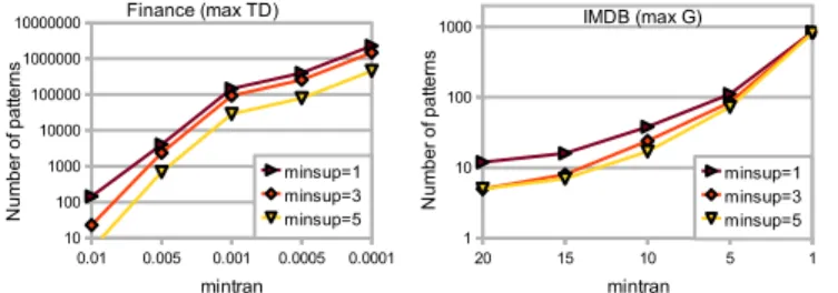
Figure 10:Number of solutions when enforcing different support constraints
Q3: What is the importance of thresholds: Figure 10 shows the number of solutions for different thresholds on the minimum number of actors (IMDB) and districts (Finance), which corresponds to a minimum support threshold as common in traditional conjunctive query mining. Increasing this threshold results in the expected behavior of reducing the number of patterns found. However, more importantly, these results show that the impact of themintranthreshold is much larger than that of the minsup threshold, again showing the usefulness of this additional constraint.
Q4: Do we find interesting patterns: We validated the patterns found for the highest minstran thresholds. For the running example setting applied on the IMDB data, the best scoring pattern consists of Charlie Chaplin and Charley Chase, each having over 50 movies of type Short and Comedy. These actors are well-known in these genres. To demonstrate the generality of our approach, we also analyzed the results for the dynamic discriminative pattern mining setting (Figure 3) on the Finance data. We define two districts to be close if they are part of the same region; we uniformly sample an equal number of transactions per district to avoid finding patterns that compare large dis-tricts with small disdis-tricts. The approach found all patterns under a minsup = maxsup = 141 constraint in 257 seconds. Example patterns found include that over 15% of transactions in the Plzeˇn-sever district performed a credit transaction with a balance over 54500, while in the nearby Karlovy Vary district this was only the case for less than 5% of the transactions; as well as that in the South Moravia region the ˇZ´ar nad S´azavou district has only half as many credit transactions as the Znojmo district, while having more than triple the amount of cash withdrawals compared to the Hodonin district.
VII. CONCLUSIONS ANDFUTUREWORK
In this paper we introduced a setting for constraint-based pattern mining in multi-relational databases. Compared to earlier approaches, it does not search for conjunctive queries but treats the pattern mining problem as a constraint satis-faction problem. The benefit of this is that it allows the integration of constraints over multiple relations, including closedness and maximality constraints. We verified exper-imentally that the proposed approach allows to find new types of patterns and can be used to find smaller numbers
of patterns effectively.
Many possibilities for future work remain. First, we re-stricted ourselves to binary relations. Higher order relations, which correspond to tensorsin the data mining community, could also be of interest in some applications; a further question of interest is here how propagators for higher order relational consistency [14] relate to those used in a data mining context [13]. A second question of interest is how to bridge the gap between conjunctive query mining systems and our approach. As at a high level the constrains in our approach correspond to atoms in conjunctive queries, a possibility is to perform a search over sets of constraints, similar to the search procedures used by conjunctive query mining systems to construct queries. Finally, extensions of the framework towards more complex constraints should be relatively easy, such as degree constraints relative to the number of selected objects, correlation constraints and other aggregates than count aggregates.
Acknowledgements. This work was supported by a Postdoc and project “Principles of Patternset Mining” from the Research Foundation—Flanders, as well as a grant from the Agency for Inno-vation by Science and Technology in Flanders (IWT-Vlaanderen).
REFERENCES
[1] R. Agrawal, H. Mannila, R. Srikant, H. Toivonen, and A. I. Verkamo, “Fast discovery of association rules,” inAdvances in Knowledge Discovery and Data Mining, 1996, pp. 307– 328.
[2] L. Dehaspe and H. Toivonen, “Discovery of frequent Datalog patterns,” in Data Mining and Knowledge Discovery, vol. 3. Kluwer Acadamic Publishers, 1999, pp. 7–36.
[3] S. Nijssen and J. N. Kok, “Efficient frequent query discovery in FARMER,” inPKDD, 2003, pp. 350–362.
[4] B. Goethals and J. Van den Bussche, “Relational association rules: Getting warmer,” inPattern Detection and Discovery, 2002, pp. 125–139.
[5] A. J. Knobbe, A. Siebes, and B. Marseille, “Involving ag-gregate functions in multi-relational search,” inPKDD, 2002, pp. 287–298.
[6] L. De Raedt, T. Guns, and S. Nijssen, “Constraint program-ming for itemset mining,” inKDD, 2008, pp. 204–212. [7] F. Rossi, P. Van Beek, and T. Walsh,Handbook of Constraint
Programming. Elsevier, 2006.
[8] F. A. Lisi and D. Malerba, “Efficient discovery of multiple-level patterns,” in SEBD, 2002, pp. 237–250.
[9] A. Jim´enez, F. Berzal, and J.-C. Cubero, “Using trees to mine multirelational databases,”Data Mining and Knowledge Discovery, pp. 1–39, 2011.
[10] G. Garriga, R. Khardon, and L. De Raedt, “On mining closed sets in multi-relational data,” inIJCAI, 2007, pp. 804–809. [11] Y. Jin, T. M. Murali, and N. Ramakrishnan, “Compositional
mining of multirelational biological datasets,” ACM Trans. Knowl. Discov. Data, vol. 2, pp. 2:1–2:35, April 2008. [12] F. Afrati, G. Das, A. Gionis, H. Mannila, T. Mielikainen, and
P. Tsaparas, “Mining chains of relations,” inICDM. IEEE, 2005, pp. 553–556.
[13] L. Cerf, J. Besson, C. Robardet, and J.-F. Boulicaut, “Closed patterns meet n-ary relations,” ACM Trans. Knowl. Discov. Data, vol. 3, pp. 3:1–3:36, March 2009.
[14] C. Bessiere, “Constraint propagation,” in Handbook of con-straint programming. Elsevier, 2006.