Essays on persistent management skill

(1)

c

(2)

ESSAYS ON PERSISTENT MANAGEMENT SKILL

BY XIN LI

DISSERTATION

Submitted in partial fulfillment of the requirements

for the degree of Doctor of Philosophy in Agricultural and Applied Economics in the Graduate College of the

University of Illinois at Urbana-Champaign, 2016

Urbana, Illinois

Doctoral Committee:

Associate Professor Nicholas Paulson, Chair, Co-director of Research Professor Gary Schnitkey, Co-director of Research

Associate Professor Mindy Mallory Professor Nolan Miller

(3)

Abstract

This is a comprehensive study of farm management performance. The rapid growth of farm income and production costs has raised both new questions and warranted revising old questions; these in-clude the existence of persistent management skill, the management strategies and profitability, farm growth and the land investing behavior associated with farm wealth. To address these ques-tions, farm management performance is analyzed based on yearly Illinois Farm Business Farm Management (FBFM) panel data across 9,831 farms from 1996 through 2014.

Agricultural producers operate in a volatile environment, facing a number of sources of risk. A key question is whether farmers who are more highly skilled can better mitigate these risks and consistently earn higher returns than their lower skilled peers. Two out-of-sample tests of skill persistence are used to analyze the ability of farm managers that consistently perform well over yearly and longer time horizons. The results suggest that the most skilled managers often generate better financial results and that management skills are consistent and predictable. Furthermore, the top 10% of farmers have substantial ability to persistently perform.

The alpha scores (or skill estimates) for farm managers are analyzed to determine if most prof-itable farmers possess specific skills or knowledge against adverse events in a volatile environment. This study emphasizes the strategic and operations aspects of managing a farm. Farms are eval-uated under different scenarios of management skill portfolios. Fundamental farm management basics are discussed in this study, including budgeting, production planning, financial analysis, financial management, investment analysis, and control management. Farm managers will want to consult it to improve the effectiveness, objectivity, and success of their decisions.

(4)

concentration. The study analyzes the factors underpinning this prominent trend. It has crucial policy implications because theory would suggest high profit farms should capture the resources over time. Two important hypotheses are derived and tested using dynamic growth model and choice behavior model: 1) farms that expand the most are more profitable; 2) returns have systemic influence on the rental and accumulation decision and hence upon the land tenure. Results suggest that high profit is often touted as a motivation factor for land investing. An innovative aspect of this study is that it brings together qualitative, quantitative, and institutional sources of information to paint a more complete picture of farm growth in the United States.

(5)

(6)

Acknowledgements

It is a pleasure to take a few moments and remember all of the support and assistance that I received as I worked on this dissertation. Friends, family, teachers, and many others have sustained me through the process.

This is a great opportunity to express my respect and gratitude to my advisor, Dr. Nicholas Paulson, who has provided me with support and guidance throughout my graduate career. I espe-cially thank him for the abundance of patience he possesses and continues to show for my educa-tion, professional growth, and advancement in writing skill. Also, I would like to express a special thanks to Dr. Gary Schnitkey who helped me learn how to really “think”. He provided countless hours of support to make these essays possible and contributed substantially to my professional growth. I am pleased to thank Dr. Mindy Mallory and Dr. Nolan Miller for providing thoughtful comments and agreeing to actively participate as part of my dissertation committee. I also would like to acknowledge all those in my personal life who supported me through this process. Special thanks are granted to my parents who have shown unwavering support of my educational pursuits. Lastly and most importantly, I offer my thanks to all my dear friends, for without them none of this would be possible.

(7)

List of Tables

2.1 Descriptive Statistics . . . 30

2.2 Spearman Rank Correlations . . . 31

2.3 Contingency Table . . . 32

2.4 Spearman Rank Correlations . . . 33

2.5 Contingency Table . . . 34

2.6 Farm manager performance evaluation, 1996-2014 . . . 35

2.7 Transition table, 1996-2014 . . . 36

3.1 Summary Statistics, 1996 through 2014 . . . 59

3.2 Alpha estimates for farms with 10 more years of data available . . . 60

3.3 Short-term (Cross-sectional Regression) Profitability Evaluation, 1996-2014 . . . . 61

3.4 Long-term (Time-series Regression) Profitability Evaluation, 1996-2014 . . . 62

3.5 Short-term (Cross-sectional Regression) Crop Yields, 1996-2014 . . . 63

3.6 Long-term (Time-series Regression) Crop Yields, 1996-2014 . . . 64

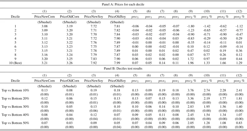
3.7 Short-term (Cross-sectional Regression) Prices Received, 1996-2014 . . . 65

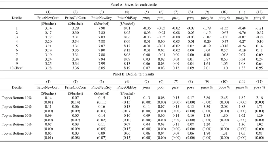
3.8 Long-term (Time-series Regression) Prices Received, 1996-2014 . . . 66

3.9 Short-term (Cross-sectional Regression) Non-land Costs Structure, 1996-2014 . . . 67

3.10 Long-term (Time-series Regression) Non-land Costs Structure, 1996-2014 . . . 68

3.11 Short-term (Cross-sectional Regression) Land Costs, 1996-2014 . . . 69

3.12 Long-term (Time-series Regression) Land Costs, 1996-2014 . . . 70

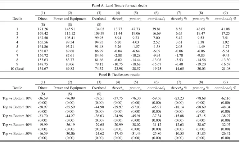
3.13 Short-term (Cross-sectional Regression) Land Tenure, 1996-2014 . . . 71

3.14 Long-term (Time-series Regression) Land Tenure, 1996-2014 . . . 72

3.15 Short-term (Cross-sectional Regression) Farm Characteristics, 1996-2014 . . . 73

3.16 Long-term (Time-series Regression) Farm Characteristics, 1996-2014 . . . 74

3.17 Short-term (Cross-sectional Regression) Liquidity Evaluation, 1996-2014 . . . 75

3.18 Long-term (Time-series Regression) Liquidity Evaluation, 1996-2014 . . . 76

3.19 Short-term (Cross-sectional Regression) Solvency Evaluation, 1996-2014 . . . 77

3.20 Long-term (Time-series Regression) Solvency Evaluation, 1996-2014 . . . 78

3.21 Short-term (Cross-sectional Regression) Asset Turnover Ratio, 1996-2014 . . . 79

3.22 Long-term (Time-series Regression) Asset Turnover Ratio, 1996-2014 . . . 80

3.23 Short-term (Cross-sectional Regression) Operational Expense Ratio, 1996-2014 . . 81

3.24 Long-term (Time-series Regression) Operational Expense Ratio, 1996-2014 . . . . 82

4.1 Summary Statistics, 1996 through 2014 . . . 114

(10)

4.3 Average Profitability Measurement, 1996 through 2014 . . . 116

4.4 Farms with Significant Alpha Estimates . . . 117

4.5 AB Estimates (all variables in first differences), 1996 through 2014 . . . 118

4.6 Probit Model Estimates for Total Farm Size, 1996 through 2014 . . . 119

4.7 Probit Model Estimates for Cash Rented Land Size, 1996 through 2014 . . . 120

4.8 Probit Model Estimates for Owned Land Size, 1996 through 2014 . . . 121

4.9 Multinomial Probit Estimates, 1996 through 2014 . . . 122

4.10 AB Estimates (farms present for more than 10 years), 1996 through 2014 . . . 123

4.11 Probit Model Estimates (farms present for more than 10 years), 1996 through 2014 124 4.12 Probit Model Estimates (farms present for all years), 1996 through 2014 . . . 125

4.13 AB Estimates, 1996 through 2005 . . . 126

4.14 Probit Model Estimates, 1996 through 2005 . . . 127

4.15 AB Estimates, 2006 through 2014 . . . 128

4.16 Probit Model Estimates, 2006 through 2014 . . . 129

A1 One-year Spearman Rank Correlations . . . 142

A2 One-year Contingency Table . . . 143

A3 Four-year Spearman Rank Correlations . . . 144

A4 Four-year Contingency Table . . . 145

(11)

List of Figures

2.1 Probabilities of subsequent annual skill rankings given initial rankings for farm

managers, 1996-2014 . . . 37

3.1 Number of Farms Participating in FBFM Records for Different Time Horizons . . 83

3.2 Plots of key variables, 1996-2014 . . . 84

3.3 Economic efficiency of various land tenure systems . . . 85

3.4 Economic efficiency of various farm characteristics . . . 86

4.1 Plots of key variables per region, 1996-2014 . . . 130

4.2 Distributions of net farm income, 1996-2014 . . . 131

4.3 Distributions of farm size, 1996-2014 . . . 131

4.4 County average ratios . . . 132

4.5 Density plots for two groups of farms, 1996-2014 . . . 133

4.6 Land tenure changes for two groups of farms, 1996-2014 . . . 134

D.1 Total Land Size Growth Rates, 1996-2014 . . . 169

D.2 Total Cash Rented Land Size Growth Rates, 1996-2014 . . . 170

(12)

Chapter 1 Introduction

Good management is a crucial factor in the success of any business. Farms are no exception. To be successful, farm managers will make and execute the accurate decisions. The long-term di-rection of a farm is determined through strategic planing. This is because production agriculture in the United States and other countries is changing along the following lines: more mechaniza-tion, increasing farm size, continued adoption of new technologies, growing capital investment per worker, more borrowed or leased capital, new marketing alternatives, and increased business risk. These factors create new management problems, but also present new opportunities for managers with the right skills.

The complex issues agriculture is facing today, such as climate change, food and energy sup-ply, globalisation of markets, population and economic growth and scarcity of natural resources, have drawn much deserved public attention to farm-related behavior and risk factors. For in-stance, after softening in the recent recession, surging farm revenues fueled a sharp rebound in U.S. farmland values. Stronger economic activity in emerging countries, especially China, led to stronger-than-expected global export activity. All of these new issues call for approaches that integrate knowledge of farm management decisions across a wide range of fields, including land allocation, size adjustments and intensity of production subject to available technologies as well as farm resources. These decisions occur regularly and are highly relevant for the overall impact of policies on the agricultural system, because the implied change in the distribution of farm structure not only affects the farm incomes and farm asset values, but also changes aggregate production at market level. Therefore, by taking a closer look at today’s farm performance, an assessment ex-ercise may improve the validity of the calculated social policy impacts from the relevance for

(13)

economic indicators.

For decades, the dominant trend in U.S. agriculture at the farm level has been towards greater concentration. The large farms and contract operations have grown in numbers while the number of mid-sized independent family farms has shrunk. The changing structure of farmland ownership has important consequences for equity within agriculture and thus has been the subject of considerable interest among agricultural economists and policy makers.

In recent years increasing attention has been paid to the rising land values, cash rents, and the other costs of production, which could limit profits and raise risk profiles. With soaring farmland values, questions naturally arise about the capacity of current farm income to support such high land costs. Farmland occupies a uniquely important role in the performance of the agricultural sec-tor. Agricultural uses large areas of land, distinguishing it from most other industries. Specifically, farm real estate accounts for 85% of the total value of all farm assets and serves as the primary source of collateral in production loans. Motivated by this increased role of farmland market and interactions with other existing uncertainties in farm operations, this dissertation considers the im-portant decisions of how much land to control and how to acquire it, in relation to identifying effective and persistent farm management skills.

Two factors driving farm performance can be distinguished: agri-environmental conditions and farm management strategies. The probably implicit choice for adoption of a strategy may be governed by agri-environmental conditions (e.g., soil quality, altitude, climate, rainfall and access to water) beyond the farmer’s skills and objectives. An interesting question is raised whether agri-environmental factors are a curse or a blessing to a farm manager. Environmental factors have been seen as the unobservable variables from assessments of economic efficiency. However, to increase the value of farm output, productive and effective management strategies are still largely required. For instance, regarding soil fertility, farmers need to increase high quality nutrient inputs at low cash and labor costs to the farmer. Although most research determine that natural endowment or weather conditions can have direct influence on farm performance, they do not directly calculate if farm managers successfully profit from their farming skills or natural resource endowment.

(14)

Moreover, while numerous studies have presumed that skill does lead to better performance and higher returns, the measurement of intrinsic skill has been conspicuously absent. The lack of attention in the literature to date is due in part to difficulties in developing suitable data series for farmers’ financial performances in which measures of skill effects could likely be detected, and in controlling for non-operator influences, such as farm characteristics, in farm returns. The aim of this dissertation is to fill this gap in the empirical analysis of persistent management skills by simultaneously investigating management strategies, farm growth, and structural change for a panel of 9,831 farm households in Illinois for the period from 1996 to 2014.

This dissertation is composed of three essays (chapters) and derives its motivation specifically from financial performance and management skills in agricultural sector. The theme of the papers is focused on the examination of farm management skill persistence and critical land accumulation decision related to farm income growth. The relationships among the three essays are as follows. The first essay answers the question “if there are persistently skilled farm managers”, while the second essay studies the means and patterns of how these managers operating the farm by applying alpha scores (skill estimates) to decoding farm management patterns. The third essay sheds light on the implications of the first two essays for the role of land accumulation decisions. Specifically, this essay analyzes farm income concentration that restrain small farm operators from making high incomes and focuses on farmer’s land control and use.

An underlying assumption by many in a number of studies of farm performance is that the best have different management styles and strategies. The goal of the first essay (chapter 2) is to explore if there are farmers who outperform their peer group on a persistent basis. Getting a fundamental understanding of persistence-based management behavior is important because agricultural pro-ducers are crucial to the fundamental economy of the U.S., contributing to major production and employing more than one sixth of the work force in the U.S.1 In addition, production agriculture has certainly not been immune to crises - the farm crisis in the 1920s and later in the 1980s, and 1_{U.S. USDA. National Agricultural Statistics Service.} _{2007 Census of Agriculture.} _{N.p., 15 March}

2011. Web.http://www.agcensus.usda.gov/Publications/2007/Online_Highlights/Fact_

(15)

the most recently 2008 financial crisis among others. Every year, the U.S. government spends billions of dollars on funding to provide safety nets for agricultural producers, since these pro-ducers operate in a volatile environment, facing a number of sources of risk. Some risks, such as commodity and input price volatility, can be more easily managed than others through finan-cial instruments. However, certain supply-and-demand dynamics are truly driven by exogenous forces such as weather, disease, and macroeconomic conditions. It is implausible and impractical to provide a hedge against these types of risk. The above issues underscore the need for a long-run perspective on farm management skills, as managers whose financial performance was superior in one economic environment could experience difficulties in another.

While it is easily accepted that better farm management styles with higher revenue are distinct from those with poor performance, little effort has been made in the empirical literature to incorpo-rate managerial skill persistence into analysis of farm performance. Since little formal research has addressed this crucial issue in terms of skill persistence, the first paper focus on the key question “whether farmers who are more highly skilled can better mitigate multiple risks and consistently earn higher returns than their lower skilled peers”. This paper is the first, among the existing lit-erature on the management skill, to look into this gap. Different than the previous litlit-erature, the sample uses long-term farm-level survey records. Persistence is the key feature, because anyone could have large returns over short horizons only due to luck. A common approach to separate out luck from skill is to test for persistence. Persistent performance over time should be the real measure of whether or not management skills matter in agriculture. The testing approach applies well known methods used in financial literature. Overall results provide compelling evidence that the superior managers survive and are not an artifact of luck.

The second essay is provided in chapter 3 and expands the first essay in management per-sistence by documenting explanations for strategic planing and decisions to generate high farm income. The approach implemented in this chapter provides a standard empirical framework for investigating the systematic relationship between management skills and profit. This study con-tribute to the farm performance literature in two ways. First, to examine the question whether most

(16)

skilled farms have different management strategies and characteristics, the analysis constructs a comparative statistical way to compare individual farm alphas (or skill estimates). Statistical pro-cedures are used to test for strategy difference and economic efficiency in farm performance using individual farm alphas over long-term horizons. Therefore, productive and effective management skills are not an unrevealed innate quality anymore; good management skills can be cultivated, developed and learned through farm performance investigations. Second, the study also provides statistical analysis to address the question of whether the economic efficiency of top managers is on the cost side, the revenue side, or both. Fundamental farm management basics are discussed, including budgeting, production planning, financial analysis, financial management, investment analysis, and control management. Farm managers will want to consult it to improve the effective-ness, objectivity, and success of their decisions.

The third essay (chapter 4) specifically focuses on land accumulation decision. Compared with other production inputs, land is purchased infrequently and usually involves a large, long-term financial obligation. How much land to control and how to acquire it can be two of the most difficult decisions confronting farm operators. Errors made at this point may plague the business for many years. They must evaluate investments and make decisions based on present conditions with appropriate allowances for future anticipation. Land control means undoubtedly relates to farm growth and profit persistence, as rising land values, cash rents, and the other costs of production could limit profits and raise risk profiles. The land control decision is especially critical today, when many are questioning the ability of farm income to support current land values at relatively “normal” commodity prices.

A farmer’s decision model is used to show if the relationship between profits and farm size prevails. Specific case situations are analyzed by comparing profitable farms and their peer group. Since funding issues for major lenders and the emerging regulatory design arise from commod-ity and farm-related credit market activcommod-ity during the recent financial crisis, lenders and investors will be interested in the degree to which farm profitability influence tenure and investment behav-ior. Thus, potential profit growth and land accumulation dynamics need to be recognized in risk

(17)

management activities.

The dissertation contributes to the agricultural literature by providing a unique insight into the management skill and a comprehensive assessment of profitability and skills. The results are interesting to regulators who are concerned about farm leasing systems and farmland market, which helps to determine the ability of farms to invest and grow, with effects on boom/bust cycles in farmland market and total production levels. Understanding the links between farm profitability, management patterns, and land accumulation will help government to better evaluate the effects of its policies on farmland, government programs and economic growth. The theoretical framework, data, methods to be employed, and results for each of the three dissertation essays follow.

(18)

Chapter 2 Is Farm Management Skill Persistent?

2.1 Introduction

Agricultural producers operate in a volatile environment, facing a number of sources of risk. Due to the recent increase of commodity price volatility, U.S. net farm income was estimated to decline 36 percent in 2015 which could be the largest drop since 1983 (USDA, Economic Research Service)1_. In addition, production agriculture has certainly not been immune to crises. The recent financial crisis has had a direct impact on the growth of farm income and farmland values (Paulson & Sherrick, 2009; Ellinger & Tirupattur, 2009). Furthermore, new farmers are in short supply, and this problem constitutes a threat to U.S. agriculture and the food supply (Gale, 2003; Hoppeet al. , 2007). Some risks, such as commodity and input price volatility, can be more easily managed than others through financial instruments. However, certain supply-and-demand dynamics are truly driven by exogenous forces such as weather, disease, and macroeconomic conditions. It is implausible and impractical to provide a hedge against these types of risk. The above issues underscore the need for a long-run perspective on farm management skills, as managers whose financial performance was superior in one economic environment could experience difficulties in another.

A key question is whether farmers who are more highly skilled can better mitigate these risks and consistently earn higher returns than their lower skilled peers. While numerous studies have presumed that skill does lead to better performance and higher returns (Sonkaet al., 1989; Plumley 1_{2015 Farm Sector Income Forecast (USDA, Economic Research Service)}

(19)

& Hornbaker, 1991; Mishra et al., 1999), the measurement of intrinsic skill has been conspicu-ously absent. The lack of attention in the literature to date is due in part to difficulties in developing suitable data series for farmers’ financial performances in which measures of skill effects could likely be detected, and in controlling for non-operator influences, such as farm characteristics, in farm returns. Only Urcola et al. (2004) use corn yield data from McLean County, Illinois to test whether farming skills influence yields with a focus on short-term performance. Their results support the hypothesis that farmer skill influences yields. The prior research’s sample however, is limited to only one county in Illinois, which does not consider different regions of the state.

Since little formal research has addressed this issue in terms of skill persistence, this article explores that if there are farmers who outperform their peer group on a consistent basis. Persistence is the key feature in this study, because anyone could have large returns over short horizons only due to luck. A common approach to separate out luck from skill is to test for persistence. Persistent performance over time should be the real measure of whether or not management skills matter in agriculture. The testing approach for this research applies well known methods used in financial literature (Eltonet al. , 1987; Malkiel, 1995; Carhart, 1997; Aulerichet al., 2013) to see if some managers consistently outperform other managers.

Management skill persistence is well documented in the finance and marketing service litera-ture with mixed results. For instance, Carhart (1997) finds persistence in mutual fund performance does not reflect superior stock-picking skill. Rather, common factors in stock returns and persistent differences in mutual fund expenses and transaction costs explain almost all of the predictability in mutual fund return. Grinblattet al. (1995) find that momentum strategies generate better perfor-mance persistence. This is in contrast to Carhart (1997), who finds that transaction costs consume the gains from following a momentum strategy in stocks. These results are sensitive to model specification. Extensive literature also exists on investment performance in the mutual fund and hedge fund industries (Grinblatt & Titman, 1992; Kosowskiet al., 2006). This literature focuses on the performance of an entire portfolio relative to market benchmarks. Although the results are not easily compared to this analysis, similar methods in measuring performance persistence can

(20)

be used in the agricultural context. The research by Irwin et al. (2006) and Cunningham et al. (2007), suggest that pricing performance of agricultural market advisory services is unpredictable.

While it is easily accepted that better farm management styles with higher revenue are distinct from those with poor performance, little effort has been made in the empirical literature to incor-porate managerial skill persistence into analysis of farm performance. There are two purposes for investigating longer-run farm performance across a large pool of data: first, to find evidence of per-sistent managerial skill explained by readily observable data and proxies for managerial attributes; second, to ascertain if significant differences in performance can be documented for a large group of relatively homogeneous farms by considering performance over time.

This study expands the existing literature in farm management by controlling for survivor bias, and by documenting common-factor explanations for farm performance persistence. Section 2 presents models of performance measurement on the appropriate benchmark. Section 3 discusses the data set corrected for survivor bias. Section 4 documents and explains the persistence in man-agement skill and further examines and explains performance for top and bottom managers. Sec-tion 5 provides summary and conclusions.

2.2 Theoretical Model

2.2.1 Performance Measurement

The first step is to find the absolute dollar value for operating profit. Operator and land returns represent a return to both owning and operating the farmland (Schnitkey, 2010). I define operator and land return as follows:

OpRetit($/acre) = P ×Yit−Cit+LCit Acrtili = Revit−Cit+LCit Acrtili ,

where OpRetit is operator and land return per acre ($/acre) on farm ifor time period t, P is

(21)

gross sales plus net change in inventory and capital accounts);Citis the total cost (all expenses for

items purchased, payments to supplies for feed, seed, fuel, rent to owner for rented land, interest paid, unpaid labor and the value of family labor, annual depreciation, etc.);LCit is the total land

cost;Acrtili is the farm size measured by tillable acre.

Land cost is added back to net farm income from operations to eliminate the effect of land cost on operating profit. This allows the operating profit to focus strictly on the profit made from producing crops without regard to the amount of land cost, which can vary substantially from farm to farm. Eliminating this variable permits a valid comparison of this return across different farms. To recognize the unpaid labor and the value of family labor contributed to earning the profit, their opportunity costs are subtracted. This makes the results comparable to those from business where all labor is hired, as these expenses have already been deducted in the computation of net farm income from operations. Management is therefore considered the residual claimant to net farm income.

Some managers are able to generate more production or use fewer resources than their peers because they use their resource more efficiently. A general definition for efficiency is the quantity or value of production achieved per unit of resource employed. The use of OpRetit as a sole

accounting performance measure, however, is a dollar amount and does not accurately reflect use of inputs. Management on the farm can be measured by the ability of the farmer to optimize the use of natural endowments and inputs to obtain an output. Therefore, the management dimension can be embodied by input expenditures. Farm managers have direct control of these expenses and finding which critical input to manage more effectively is of interest to understanding the persistence of performance. Consequently, input variables are used as determinant variables of persistence. Also, the form of farm business (family owned/enterprise) can cause problems for interpretation of the performance measurement. To take the heterogeneity of the costs of different farms into consideration, I use a ratio to measure the percentage return with respect to the total cost per acre:

(22)

Ratioit(%) =

(Revit−Cit+LCit)/Acrtili

Cit/Acrtili

×100 = OpRetit(per acre) Cit(per acre)

×100.

This ratio of performance measure is used to evaluate the efficiency of managerial skill or to compare the efficiency of a number of different managers. Farms with low ratio should concentrate on improving this ratio before expanding production.

2.2.2 The “Hot Hand” Phenomenon

The key questions in this research are whether some farmers are more skilled at making man-agement decisions than others, and does this result in highly skilled managers financially outper-forming their lower skilled peers consistently? To conduct the persistence test, I apply the same procedure to returns using the models of performance proposed by past literature. These include the simple one-factor model of Jensen (1968), the three-factor model of Fama & French (1993), and the four-factor model of Carhart (1997). In the context of the present study, implementation of the multi-factor model approach involves two steps. The first step is to compute the average benchmark and then subtract the benchmark from each farm performance proxy. The second step is to apply the two-factor model to compute ordinary least square (OLS) estimated alphas (mul-tivariate generalization of Jensen’s alpha). The following theoretical model is derived from the conventional financial theory’s existing framework.

Ratioit=αi+γRatiojt+βZit+µit, (2.1)

ifγ = 1, then

Ratioit−Ratiojt =αi+βZit+µit, (2.2)

where

(23)

Ratiojt= the ratio of return to cost of countyjfor time period

t, which is normalized (assumeγ = 1held constant across time)2; αi= the constant term;

Zit= a vector of the farm characteristics, which contains soil

productivity (Sprit) and farm size (Acrtilit)3;

µit= the regression residual;

i, j, t= subscript indexes for farm, county, and year, respectively.

In this model, the county-level average measureRatiojtwas selected to minimize the impacts

of geography and weather on returns (e.g., good vs. bad weather, superior vs. inferior growing conditions). Also, the use of the county average benchmark is to control for systematic effects that affect all farms within a county in one specific year. Therefore, excess return is a relative performance measure. It removes systemic effects on returns that might impact every farmer peer group in a given year.

(Ratioit−Ratiojt)is the excess ratio;αiis the ratio left unexplained by the benchmark model.

Accounting for the variation in returns associated with farm characteristics (Zit) then allows us to

mainly focus on the effects of farm management, indicated byαi or the constant term. An alpha

greater than zero means a farm manager outperforms the expected performance (Jensen, 1968; Fama & French, 1993; Carhart, 1997; Kosowskiet al., 2006). Managerial capacities (αi) can then

measure cost management or/and profit-making capacities at the farm level.

Profitability is impacted by a number of factors, many of which are controlled to some extent by the management decisions of the farm operator. However, natural endowments, such as soil quality and favorable weather conditions, may disguise the manager’s actual capacities. There-fore, quantifying how much management and natural endowment (e.g., soil productivity) matter

2_County_j_{refers to the county which contains farm}_i_{, so that}_Ratio

jtcan be treated as a benchmark for farmi.

3_{The effects of location, weather, and precipitation on profitability are not taken into consideration similar to most}

research, because this analysis would control for these effects. The variability in temperature, and to a lesser extent in precipitation, are similar within a county. Also, these variables are not exactly linearly related to profitability so it is hard to predict the management skill in terms of functional form. Thus, I follow the method used by Sonka (1989) and control farm characteristics.

(24)

respectively in persistence is of interest. In addition, some dimensions that are not directly related to the production process may be captured by a secondary effect, such as the size of the farm. However, the effect of farm size on profitability is an issue continually analyzed and debated by agricultural economists (Purdyet al., 1997; Garciaet al., 1982; Goodwinet al., 2002). I suggest there may be increasing returns to scale for farms, and a normalized measure of profitability (i.e., net farm income per acre) may be enhanced by expanding the scale of the operation. The above discussion motivates the choice of the variables in the farm characteristic vector. Therefore, in order to gain some insights, I employ a two-factor model to measure performance.

Several financial studies, such as Grinblatt & Titman (1992) and Malkiel (1995), present strong evidence in favor of a “hot hand” phenomenon, which is when mutual funds that achieved above-average returns continue to enjoy superior performance. In order to test if some farmers have persistent performance, I need to identify “αit” for each of the farms over each time period. This

means OLS estimated alphas (using the time series of returns for each farmi) can not accomplish my goal of testing for skill persistence.

To circumvent this problem, ineach year, I estimate across-sectionregression:

Ratioi−Ratioj =β1Spri+β2Acrtili+µi, (2.3)

whereµiis the residual of equation (3), and

αi ≡Excess Ratioi−E[Excess Ratioi] =µi, (2.4)

where

Excess Ratioi =Ratioi−Ratioj,

E[Excess Ratioi] =β1Spri+β2Acrtili.

In this specification, alpha is represented by the residual of equation (3), which is the excess ratio left unexplained by the linear regression model in equation (4). An alpha greater than zero

(25)

means a farm manager outperforms the benchmark. This procedure proposed by Carhart (1997) can allow for the possibility of examining every possible ordering of farm manager in a given year. If some farmers have persistent performance, then it can be explained that they have consis-tently better skills than others. Farmers receiving above-average returns might be using a superior management skill, so finding performance persistence could help identify superior strategies. Two out-of-sample tests of persistence are used in the analysis to analyze the ability of farm man-agers that consistently perform well over yearly and longer time horizons, both of which have been widely applied in studies of market performance (Eltonet al., 1987; Malkiel, 1995; Carhart, 1997; Irwinet al., 2006).

2.2.3 Spearman Ranking Test

The first test is the Spearman ranking test, which is a paired correlation analysis across adjoining periods4_{. Persistence simply means that the actual statistic is correlated from one period to the} next throughout the sample periods. For instance, if financial performance of farm istatistically outperformed the benchmark in 1996, it would be correlated highly with the good performance in 1997. Therefore, for a single farm manager, whether alpha rankings in consecutive periods are positively correlated would be a measure of persistence which means the statistic is indicative of skill. Also, performing the Spearman nonparametric test on the rank ordering of performance mea-sure has some statistical advantages, for instance, it does not assume a linear relationship between variables. Correlations are calculated using pairwise deletion of observations with missing values due to an unbalanced data set. I use casewise deletion, where observations are ignored if any of the variables are missing. Here, the null hypothesis is that the performance measure is randomly ordered.

4_{Spearman (1904) rank correlation is calculated as Pearson’s correlation coefficient computed on the ranks and}

average ranks (Conover, 1980). The significance is calculated using the approximation: p = 2 ×ttail(n−

(26)

2.2.4 Winner and Loser Ranking Test

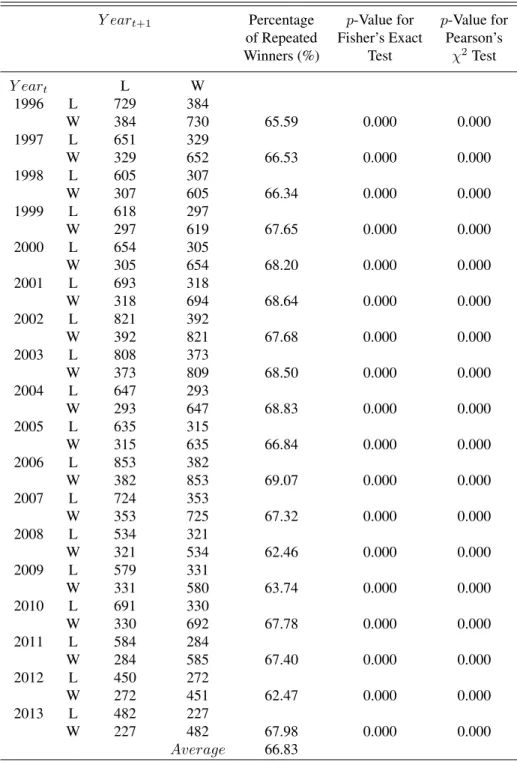
Mirroring the previous discussion, the second test is a winner and loser ranking test that assesses, in a nonparametric context, whether managers in the top half of the alphas distribution in a time period continue in the top half of the distribution in the next period. Farms with high past alphas demonstrate relatively higher alphas and expected returns in subsequent periods. The null hypoth-esis is the past ranking of a farm manager does not help predict the manager’s future ranking.

This test is based on placing farm managers into winner and loser categories across adjacent pairs of years. The first step in this test procedure is to form the sample of all farm managers that are present in the pair of years. The second step is to rank each farm manager in the first year of the pair (e.g., t = 1996) based on alpha estimates. Then, the managers are sorted in descending rank order. The third step is to form two groups of mangers in yeart: a winner is defined as a

manager’s alpha ranking that has achieved above the median; a loser is defined as a manager’s alpha ranking that has achieved below the median. The fourth step is to rank each farm manager in the subsequent yeart+1 of the pair (e.g., 1997) based on alpha estimates and once again form

winner and loser groups of farm managers. The fifth step is to compute the following category counts for the farm managers in the pair of years: winnert−winnert+1, winnert−losert+1,

losert −winnert+1, losert−losert+1. The sixth step is to construct a 2×2contingency table

formed on the basis of winner and loser counts. The appropriate statistical test in this case is Fisher’s exact test, a nonparametric test that is robust to outliers because both row and column totals are predetermined in the contingency table. The null hypothesis is that the relative proportions of yeart are independent of yeart+1. With large samples, a Pearson’s chi-squared test can also be

used.

I also calculate the percentage of winners in the initial year that remain in the upper 50% in the subsequent year. If these conditional probabilities are higher than what would result from flipping a coin (randomness), they can provide predictability. The disadvantage of this repeat winners and losers approach is that it has low power to reject the null hypothesis of no performance persistence

(27)

(Cunningham III et al., 2007). A fuller description of the variables involved follows.

2.3 Data

This research requires a panel of individual and detailed farm-level data. The lack of literature is a direct result of lack of suitable data. My data set contains continuous observations for a sample of 9,831 farms in the state of Illinois over 19 years, from 1996 to 2014, collected from the Illinois Farm Business Farm Management (FBFM) survey.

The FBFM records include a variety of financial and agronomic characteristics for each cooper-ating farm operation. Participation in this farm business analysis program is voluntary; coopercooper-ating farmers pay a fee for the educational services.

The most relevant empirical study addressing individual farm managerial skill is Urcola et al. (2004), which also uses data from the FBFM. FBFM data prior to 1996 is summarized in a different manner. Due to the data change, I focus on the time period from 1996 to 2014 for this analysis. This study extends beyond the 7-year horizon used by Urcola et al. (2004). Instead, I test for persistence using a 19-year horizon. Also, the prior research’s sample is limited to only one county in Illinois, but does not consider different regions of the state. Finally, other prior studies have focused on in-sample estimates of the correlation in performance measure rather than out-of-sample estimates that are the standard in investment studies (e.g. Malkiel, 1995). An out-of-out-of-sample measure is a more stringent test of the persistence of profit in farm management.

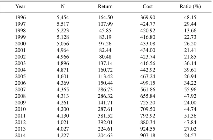
In this research, I restrict the analysis to corn and soybean farmers. Within Illinois, acreage of farms enrolled in FBFM account for approximately 25% of the acres in corn and soybean production. To be selected from a large pool of FBFM cooperator data, each farm record had to have been certified usable by the FBFM field staff representative with 180 or more tillable acres.

In this study, operator and farmland returns are computed to represent average returns to Illinois farmland5. Operator and farmland returns equal gross revenue minus non-land costs, and represent 5_{For comparison and validation, I use management return (subtracting total land costs from operator and farmland}

(28)

a return to both owning and operating the farmland6.

For each of the farms, the farm ID combined with county ID results in a unique farm iden-tification marker and is used to isolate management return ($/acre) on each farm. Ninety-eight counties in total are investigated. All FBFM expenses were adjusted for prepaid expenses, ac-counts payable and cash settlements. The enterprise analysis reports all the costs related to each farm for a given year. Total costs can be further broken down into three categories: 1) direct costs include fertilizer, seed, pesticides, drying, and storage; 2) power costs include machinery repairs, equipment depreciation, machine hire and lease, and fuel; 3) overhead costs include land, hired labor, building repairs and deprecation, insurance, and interest. In the dataset, revenues include crop revenue, livestock revenue, custom revenue and other revenue. Total gross revenue after the total cost is the net farm income7_.

FBFM reports a soil productivity ratio (SPR) based on maps of soil types for each Illinois farm, following Fehrenbacher et al. (1978). The SPR is an average of yield potential on a farm weighted by the soil types within the farm. The SPR ranges from 40 to 100, with 100 being the most productive soil quality, and was calculated at the farm level based on soil structure and quality as well as suitable crops. It directly embodies the potential productivity of the soil for main crops like soybean and corn. Therefore, the expected effect on returns should be positive as better soil should not need more use of chemicals to compensate for deficiencies.

Total tillable acres for each farm are the indicators of farm size. While Purdy et al. (1997) show that larger farms outperformed smaller farms in Kansas, Garcia et al. (1982) do not find any significant relationship between size and success. In this research, it is hypothesized that persistent

very similar (see Appendix).

6_{The return to farmland varies depending on whether the farmland is owned, share rented, or cash rented. If}

farmland is cash rented, subtracting the cash rent from operator and farmland returns yields the return to farming while the cash rent represents the return to the land ownership.

7_{The costs and returns are matched up to the same crop/calendar year. But I also noticed they may not be matched}

up to the same production/marketing year. For instance, corn that is harvested in October of one year may not be sold until the following calendar year or longer. This says that returns may have various components which could include the returns to storage. Similarly, inputs for the next production cycle which begins with planting in May may be purchased immediately after the last harvest (between October and December) rather than in the year that it is going to be used. Since the FBFM data account for the accrual management return within calendar year by recording both old crop and new crop, which means marketing/production year returns are adjusted for each year on an accrual basis.

(29)

high-return farms produce more acres than other farms.

It is possible that farmers with low skills are naturally eliminated from my database as their farms go out of business. This might create substantial survivorship bias, leaving only highly skilled farmers who are able to maintain high returns through time. Survivorship bias would likely cause an overstatement of returns obtained by farmers, a consequence of tracking only farms that remain in business at the end of sample period. Thus, survivorship bias is an important issue in mutual fund research (Brown et al. , 1992; Malkiel, 1995; Carhart, 1997; Carpenter & Lynch, 1999) since it is typical of mutual fund and hedge funds databases. However, my sample is, to my knowledge, the largest and most complete survivorship-bias-free farm database currently available. I find that the comparison of mean returns of farmers present in all years and the whole group of farmers imply that survivorship bias effects have no great differences in returns8_{. The sample is} stable with an average attrition rate of 18.1% and an average entry rate of 20.6%. According to a private conversation with FBFM specialist Bradley Zwilling, “if farms are FBFM cooperators, they are always in the data set, just not always certified useable.” So common reasons for the “attrition rate” would be that their farm has a critical error in the data and it is not certified useable. For instance, this could be due to not turning in their data, not have completing their records, etc. Urcola et al. (2004) use a similar database obtained from FBFM to study the effect of farmer skills on yields. The sample in their study is stable with an average attrition rate of 6.9% and an average entry rate of 5.8%. In addition, the comparison of mean yields of farmers present in all years and the whole group of farmers imply that survivorship bias effects can be considered negligible.

As a check on the representativeness of the sample, a number of previous studies compare the financial characteristics of farm management association members to a random sample of farms (Mueller, 1954; Olson & Tvedt, 1987; Gustafsonet al., 1990; Andersson & Olson, 1996; Kuethe et al., 2014). The earliest published study by Mueller (1954) find that, compared to a random sam-ple, managerial ability is not greatly different on farms in the FBFM service and record-keeping farms given equal basic resources, particularly farm size and soil quality.

(30)

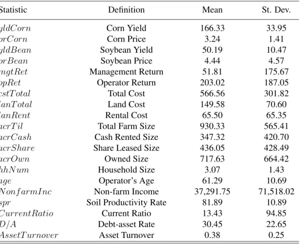
Table 2.1 reports descriptive statistics of the farm data. My sample includes a total of 9,831 diversified farms over 19 years. The data set was cleaned by omitting the outliers. I used a simple rule of thumb, z = 3 guideline (i.e. data points three or more standard deviations from the mean ofReti), as an initial screening tool, and depending on the results of that screening, examined the

data more closely and modified the outlier detection strategy accordingly. The sample includes 50,623 total observations with per acre average return of $26.22 and average expenses of $553.71. Total land costs include interest charge on land, taxes, cash rent and leasing cost. Farms in this report have per acre average land costs of $150.13 and per acre average operator and land return of $176.35. In addition, the county average ratio in the sample is 25.12% (the excess ratio is 0%). Also, over the full sample, average farm size is 984.72 acres and the average soil productivity index value is 79.50.

2.4 Persistence Tests

2.4.1 One-year Persistence Test

The Spearman rank correlations for alphas are shown in table 2.2. Table 2.2 shows the p-values for the null hypothesis that the past ranking of a farm manager’s alpha does not predict the manager’s future ranking (H0 : ρ = 0 versusHa : ρ > 0). Rank correlations are all significant and positive

between adjacent years. In this case, random rank-ordering is rejected. Rank correlations for alphas vary between the adjacent years and have an overall average of 0.47. Thus, results indicate that, even after controlling for soil productivity and farm size, some farmers still have consistently better skill than other farmers. However, since the Spearman test treats the ordering of winner and loser categories equally, it lacks power against the hypothesis of predictability in performance.

Table 2.3 shows the number of winners and losers conditional on the previous year’s perfor-mance based on alpha ranking. On average, the percentage of repeated winners is 66.83% (the conditional probabilities are higher than 25%,i.e.what would result from flipping a coin).

(31)

Results show the p-values for the Fisher’s exact tests of the null hypothesis that the past ranking of a manager’s skill does not predict the manager’s future ranking. The null hypothesis that a winner and loser are randomly determined is rejected in all years. These results are consistent with the conclusions of the correlation analysis shown in the previous table and support the hypothesis that a farm manager’s skill influences financial performance and persists.

2.4.2 Long-term Persistence Test

The predictability results presented so far are based on one-year comparisons. It is possible for performance to be unpredictable over longer time horizons, but predictable over shorter horizons. To reduce the noise in past performance rankings, I repeat my earlier analysis and assess longer-term predictability. The sample is again limited to all 19 crop-years of the Spearman ranking test. The correlations are the rank correlations between a producer’s average alpha in a four-year period and alpha in a subsequent four-year period (Cunningham III et al., 2007). Alpha rankings are averaged for each of the farm managers during the initial four years (e.g., 1996−1999) and the subsequent four years (e.g.,2000−2003). Tests of predictability are then applied to the two sets of long-term averages.

Results are similar for a longer-term period. Table 4 shows skill persistence in the long-term period in terms of positive rank correlation in two consecutive four-year periods. Table 5 shows the percentage of managers whose alpha ranked in the top 50% in two consecutive four-year periods. All the percentages of repeated winners in longer-term tests are higher than in the one-year tests. The Fisher’s exact tests and Pearson’s chi-squared tests results reject the null hypothesis that alpha ranking is by chance. Therefore, table 2.4 and table 2.5 suggest strong skill persistence in the long run.

(32)

2.4.3 Robustness Check

For comparison and validation, I use operator and land return, management return, return-cost-ratio, and management return to land cost ratio to test persistence, and return on farm assets. The results derived from these measurements are very similar (see Appendix).

In these data sets the residuals may be correlated across farms and across time, and OLS standard errors can be biased. Historically, there are two principle approaches to this, some-times called time-series regressions (the Fama-French method) and cross-sectional regressions (the Fama-MacBeth method). This paper also examines the time-series method used in the liter-ature (Fama & MacBeth, 1973). The intent is to provide intuition as to if the different approach gives different answers.

For time-series regressions, time-series data for each farmiare used to estimate the regression intercept αi for that farm. In this case, I estimate equation (2). I obtain an alpha for each farm

and test the significance. The reason I can use time-series regressions in this case is that the management skills are estimated as the time-series average of the excess ratio left unexplained by the factor regression model. The factor model has one implications: An alpha greater than zero means a farm manager outperforms the benchmark. Standard statistical tests can be used to test if these are positive alphas. This is equivalent to testing the intercept in the cross-sectional regressions. For the sake of brevity, I do not include results for the time-series regression results, but these support the existence of management skill and are available from the author upon request.

2.5 Performance Evaluation for Top and Bottom Managers

2.5.1 Performance Evaluation for Out-of-sample Periods

The performance evaluation method is based on placing farm managers into ten deciles across adjacent pairs of years. The first step in this test procedure is to form the sample of all farm managers that are present in the pair of years and exclude any not in both periods. The second

(33)

step is to rank each farm manager in the first year of the pair (e.g., t = 1996) based on alphas with the most skilled manager as the number one. Then, the managers are sorted in descending rank order. The third step is to form deciles of mangers inyeartbased on manager’s skill ranking.

The fourth step is to use the deciles of managers formed in yeart and compute how the same

manager performed in the subsequentyeart+1 of the pair (e.g., 1997) by profits. The fifth step is

to compute the difference in the profits between the top and bottom performing manager groups and test the null hypothesis: the difference between the top and bottom performing groups is zero. If the performance difference between the top and bottom groups is significantly different than zero using an appropriate statistical test, then the null hypothesis can be rejected and the conclusion is reached that top managers do have stellar management skills and stand out amongst their peers.

The appropriate statistical test in this case is Wilcoxon signed-rank test, a nonparametric test that is well-specified and among the most powerful in their comparison of several predictability tests for mutual funds and agricultural futures markets (Carpenter & Lynch, 1999; Aulerichet al. , 2013). The Wilcoxon signed-rank test is used when comparing two related samples, matched samples, or repeated measurements on a single sample to assess whether their population mean ranks differ (Wilcoxon, 1945). It can be used as an alternative to the paired Student’s t-test, t-test for matched pairs, or the t-test for dependent samples when the population cannot be assumed to be normally distributed (Lowry, 2014).

Table 2.6 displays the average returns for the out-of-sample yeart+1 for each decile in Panel

A. For instance, in the skill estimate (α) results the top decile is 10 and is formed based on alpha rankings for an in-sample periodt(e.g., 1996, 1997, ..., or 2013) and summing the skill estimates of those same top decile managers in the out-of-sample period t + 1 (e.g., 1997, 1998, ..., or 2014). Similarly, in the annual profit results the top decile is 10 and is formed by ranking the skill estimates for an in-sampleyeart(e.g., 1996, 1997, ..., or 2013) and summing the profits of those

same top decile managers in the out-of-sampleyeart+1 (e.g., 1997, 1998, ..., or 2014).

The out-of-sample skill estimate results are shown in column (1) in Panel A. The average α values of allyeart+1 is 79.19 for the top 10% and -104.87 for the bottom 10%. The averages for

(34)

top 10%, 20%, ..., 50% managers are significantly greater than zero whereas bottom 10%, 20%, ..., 50% managers find the results are less than zero. Managers’ skill estimates in out-of-sample periodt+ 1correspond with their rankings in the previous period, which is clearly demonstrated in the results where greater skill estimates are generated inyeart+1 among those larger decile (better

skilled managers) groups inyeart.

The out-of-sample profits are presented in columns (2) and (3) in Panel A. The average profits are quite large for top managers. The top 10% of managers show better financial performance with operator and land return (OpRet) and management return (MgtRet) of $257.55 per acre and $76.90 per acre, respectively. The bottom 10% of managers display poor performance with operator and land return and management return of $70.88 per acre and $-83.42 per acre, respectively. Results clearly suggest that superior gains is due to substantial skills of top decile managers not due to factors outside of the manager. The average profits gained in out-of-sample period monotonically increase along with the managers’ skill rankings with much larger profits achieved inyeart+1 if

one shifts from bottom decile (worst) to top decile (best) inyeart.

The profit deviation analysis is also included, which is shown in columns (4) and (5) in Panel A. The deviation is calculated based on the difference between the value ofprof iti,t and its mean

prof ittforyeart, where profit is measured in the form of OpRet or MgtRet. The purpose of

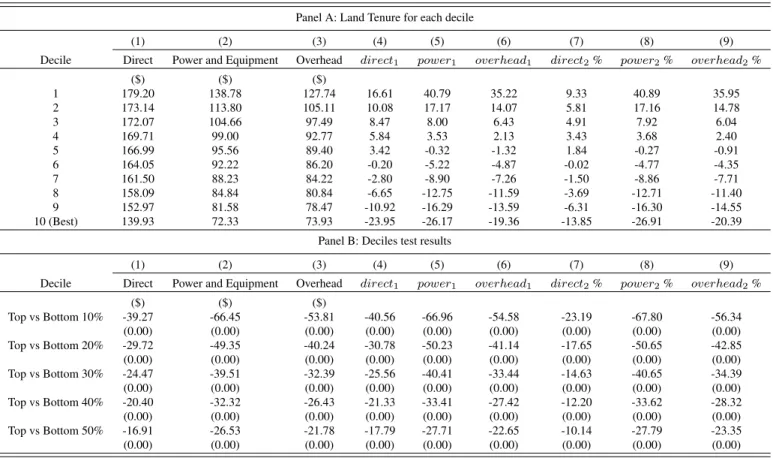
in-cluding the deviation measure is to analyze farm manager’s performance behavior in a different perspective. One may argue that the averages shown in column (2) and (3) do not capture random events happening during each time period. However, if the time effect is “fixed”, then the devia-tions will offer more compelling evidence addressing the skill persistence question. The sign of the deviation reports the direction of that difference (e.g., the deviation is positive when a farm’s return outcome exceeds the benchmark in that year) while the magnitude of the value indicates the size of the difference. For example, large deviations appear in or immediately next to top and bottom deciles with negative values shown in deciles 1-4 and positive values in deciles 5-10.

In Panel B, table 2.6 displays the difference between top and bottom deciles for the differ-ent skill/return measures and deciles test results. The difference of skill estimates between the

(35)

top and bottom decile is 184.07 which is significantly different from zero. Top managers earn $186.68 per acre more than the bottom in terms of operator and land return, and top managers ex-perience $160.33 management gains than the bottom 10%. The statistical significance of the test result that top and bottom managers performances differ prevails in every single scenario among different skill/return measurements. If one expects managers to persist in earning profits then the top/bottom out-of-sample deciles would have greater influence than the intermediate out-of-sample deciles, and this would decline as I expand from the 10% to 50% comparisons. The results are also presented for comparisons of the top and bottom 20%, 30%, 40% and 50%. For example, the difference of skill estimates between the top and bottom 50% decile is 72.10 which is significantly different from zero. Top 50% managers earn $71.49 per acre more than the bottom in terms of operator and land return, and top managers experience $59.85 management gains than the bottom 50%. The findings persist even when I expand the size of the deciles, but the differences in magni-tude decline. In sum, the top 10% of managers tend to show substantial persistence in performance at an annual horizon.

The persistence in the consecutive two years indicates that managers can focus on intermediate periods even though it may be difficult to maintain profitable position in the presence of random events which occur in agricultural markets.

The compelling performance persistence results are due to superior skills in the top decile and high profits gained by them. In sum, the top decile of managers tend to show substantial persistence in performance at an annual horizon which reconcile to the results in winner and loser test.

2.5.2 Transition Table

The second method takes into account the magnitude of skill estimate differences between top and bottom performing groups and allows for the possibility that top deciles of farm managers remain in the same decile when other midrange farm managers switch between skill categories.

The starting of the method is similar to the previous decile test. First, create the pairs of adjacent time periods and rank each farm manager in the first year of the pair based on skill

(36)

ranking. Then, form deciles of mangers in yeart. Next, use the deciles of managers formed in

yeart and compute skill rankings for the same manager in the subsequentyeart+1 of the pair and

once again form deciles of farm managers. For instance, take the most skilled decile, decile 10, in yeart and without resorting or reforming groups of managers, determine how this decile of

managers fromyeartperformed inyeart+1.

Table 2.7 displays transition tables of initial and subsequent annual skill rankings. The transi-tion occurrences and probabilities for all farm managers ranked based on their skill across deciles are presented in Panel A and Panel B respectively and graphically represented in figure 2.1. In a case where all profits are random and no persistence exists, each value in the matrix would be equal with probability 10%. In a case, where managers have persistent skills that are not due to luck and managers always rank exactly the same in every period, each probability on the diagonal (1/1, 2/2, ..., 10/10) would be 100%. The values on the diagonal indicate the probability that a farm manager will remain in their current decile, with other values indicating the likelihood of them shifting into a different decile. For example, managers in decile 10 are likely to remain in decile 10 about one third the time (probability equal to 0.34). Similarly, managers in decile 1 have a moderate chance (probability equal to 0.39) of remaining in the worst category. There is a slight chance (probability equal to 0.05) that a manager from the worst group in a given year can transit to the best group. Likewise, there is a similar small chance (probability equal to 0.04) that a manager can transit from the best group to the worst group within one year. For Panel B, the probabilities appear symmetric around the middle of the distribution with the greatest probabilities in the 10/10 and 1/1 deciles.

The highest value in each row indicates whether managers are likely to remain in their current decile rather than switching to another decile. If the highest value in each row corresponds to values along the diagonal from upper left to lower right (the probability of remaining in the same decile), then persistence is expected. Panel B shows that the highest, second and third highest values are either appear in the diagonal or immediately next to it indicating that when managers switch between categories they are likely to switch to only one decile higher or lower rather than jump across multiple categories.

(37)

All the diagonals are greater than 10% and many managers either stay in the same decile or move one decile up or down. This tendency for managers to stay in or around their decile supports the conclusions of winner and loser test which finds that skill persists among managers. Managers who are initially in decile 10 in yeart are likely to be the decile 10 in yeart+1. Overall, the

transition tables in Panel A and Panel B provide rather strong evidence that persistent skill exists among top farm managers.

However, managers who are initially in decile 1 (worst) inyeartare also likely to be the decile

1 inyeart+1. The managers in this case may fall into one of two types, those who possess no skill

and are severely challenged by the agricultural market, and those who take large risks to become financial vulnerable and exhaust their equity. Persistent performing in decile 10 (best) encourages further participation through profits, but the continued performance of those in decile 1 (worst) is surprising since managers are continually earning negative returns. It is possible that the farmer earing negative returns are still exploring if they currently don’t want to liquefy their assets (e.g., land) or they are compensating for losses with other subsidies.

Although the results from winner and loser ranking test and the top and bottom performing deciles test generally support each other, differences in interpretation exist in the statistical sig-nificance results. The purpose of the winner and loser ranking test is to investigate whether farm mangers in the top half of the distribution in a time period tend to stay in top half in the next period whereas differences in skill between the top and the bottom deciles provide support that persistent profit-making capacity exists among the top decile of managers.

The statistical significance of the winner and loser ranking tests is likely reflective of the high degree of persistence among top and bottom managers during the period, and as figure 2.1 demon-strates the ranking persistence of decile 1 (worst) and decile 10 (best). Figure 2.1 displays Panel B of the transition table of initial and subsequent annual skill rankings. A farm manager’s initial ranking inyeart is on thex-axis and subsequent ranking in yeart+1 is on the y-axis. The z-axis

is the probability of the subsequent ranking given the initial ranking. A large portion of managers who initially rank in decile 1 or 10 in the initial period stay in the same decile in the subsequent

(38)

period. This pattern becomes clear when analysing the four corner deciles and comparing the rankings that persisted (1/1 or 10/10) versus the drastically shifting rankings (10/1 or 1/10). The extreme rankings 1/1 and 10/10 are larger than 30% and the 10/1 and 1/10 shifts are smaller than 1%. The significance of the decile tests tend to be consistent across differences between the deciles studies (10%,20%,30%,40%,50%) and the winner and loser rank tests, but in light of figure 2.1 the significance in the other deciles is likely driven by the 10th decile managers not by the intermediate deciles.

2.6 Summary and Conclusions

Using individual farm-level data from FBFM from 1996 to 2014, this study investigates whether managerial skill persists in farm performance. The extent to which the skills used by farm man-agers are either efficient or not was measured by a two-factor model that includes a benchmark. The benchmark emphasis makes the model applicable to many farm types that differ in geographic location, tenure, and other structural characteristics. Given the evidence documented here, persis-tent profit-making capacity is an indication of skill. In addition, farm managers appear to benefit from natural endowment (i.e.soil productivity and farm size). Based on previous research (e.g., Malkiel, 1995; Urcola et al., 2004; Irwin et al., 2006), two basic outofsample persistence tests -a Spe-arm-an r-anking test -and -a winner -and loser r-anking test - -are ex-amined to determine whether farm managerial skill consistently performs well.

Overall results provide compelling evidence that the superior alphas of star managers survive and are not an artifact of luck. While it is difficult for farm managers to always profit, persistence emerges from the Illinois crop farms in terms of the rank correlations of alpha. The strongest evi-dence for persistence exists with Spearman’sρreaching 0.70 for four adjacent years. The findings identify significant persistence in ranking; managers in the top 50% of the profits distribution int tend to stay in upper half int+ 1. On average, 66.83% of winners are also winners in t+ 1. In addition, for both short and long horizons, the Fisher’s exact test and Pearson’s chi-squared test