The Recoverable Robust Facility Location Problem
Eduardo ´Alvarez-Mirandaa,1, Elena Fern´andezb, Ivana Ljubi´cc
aIndustrial Engineering Department, Universidad de Talca, Curic´o, Chile
bDepartament of Statistics and Operational Research, Universidad Polit´ecnica de Catalunya, Barcelona,
Spain
cDepartment of Statistics and Operations Research, Universit¨at Wien, Vienna, Austria
Abstract
This work deals with a facility location problem in which location and allocation (trans-portation) policy is defined in two stages such that a first-stage solution should be robust against the possible realizations (scenarios) of the input data that can only be revealed in a
second stage. This solution should be robust enough so that it can be recovered promptly
and at low cost in the second stage. In contrast to some related modeling approaches from
the literature, this new recoverable robust model is more general in terms of the considered
data uncertainty; it can address situations in which uncertainty may be present in any of the
following four categories: provider-side uncertainty, receiver-side uncertainty, uncertainty
in-between, and uncertainty with respect to the cost parameters.
For this novel problem, a sophisticated branch-and-cut framework based on Benders decomposition is designed and complemented by several non-trivial enhancements, including scenario sorting, dual lifting, branching priorities, matheuristics and zero-half cuts. Two large sets of instances that incorporate spatial and demographic information of countries such as Germany and US (transportation) and Bangladesh and the Philippines (disaster
management) are introduced. They are used to analyze in detail the characteristics of
the proposed model and the obtained solutions as well as the effectiveness, behavior and limitations of the designed algorithm.
Keywords: Facility Location, Two-Stage Robust Optimization, Branch-and-Cut,
L-Shaped Cuts
1. Introduction
Nowadays, we are more and more aware of the growing presence of dynamism and un-certainty in decision making. Fortunately, as the decisions become more complex, the avail-ability of modeling, algorithmic and computational tools increases as well. Facility location and allocation decisions are among the most relevant decisions in several private and public transportation contexts and they usually involve strategic and operative policies with mid and long term impacts. Precisely because of the practical relevance of these decisions, it
1Corresponding author: Industrial Engineering Department, Universidad de Talca,Merced 437, Curic´o,
is important that they incorporate the uncertainty that naturally appears during the plan-ning, modeling and operative process. Such uncertainty can be represented by different
realizations of the input data: customers that actually require a commodity or a service,
locations where the facilities can be located, the transportation network that can be used
for connecting customers with facilities, and the corresponding costs. The true values of
this data usually become available later in the decision process. In such cases a standard deterministic optimization model that considers a single possible outcome of the input data can lead towards solutions that are unlikely to be optimal, or for that matter even feasible, for the final data realization.
Supply chain management is a strategical area in which both uncertainty and facility
location are core elements. For instance, as it is pointed out in [45], supply chains are
particularly vulnerable to disruptions (intentional or accidental), imposing the need of taking into account the possible availability of depots and roads and different structures of the demand. Likewise, short-term phenomena such as fluctuations in commodity prices (such as oil) or long-term public policies (such as new toll road concessions) might lead to operational cost increases that should be considered when deciding the transportation network to be used. In another context, natural events such as tsunamis, hurricanes or blizzards can produce disastrous effects with unpredictable intensity on populated areas and on the transportation infrastructure. Countries such as Bangladesh and the Philippines are two typical examples; both of them are regularly hit by hydrological disasters such as floods and typhoons. Ac-cording to the Department of Disaster Management of Bangladesh [22], every year around 18% of the country is flooded, which produces over 5000 causalities and the destruction of more than 7 millions of homes. However, flooded areas my exceed the 75% of the country in case of severe events (as in 1988, 1998 and 2004). In the case of the Philippines, between 6 to 9 typhoons make landfall every year producing thousands of human losses and incalcula-ble urban destruction; in November of 2013, typhoon Haiyan produced 6241 causalities and material damage of over 809 millions USD [see 39]. In these examples, it is crucial to be able to count with a robust system of humanitarian relief facilities that even in the worst possible scenario can provide assistance with the quickest possible response reducing the number of human loses after the occurrence of the event.
The Uncapacitated Facility Location Problem (UFL), also referred as the Simple Plant
Location Problem, is one of the fundamental models in the wide spectrum ofFacility Location
problems [see, e.g., recent overviews presented in 23, 21]. In the classical deterministic version of the UFL one is given the set of customers, the set of locations, the facility set-up costs and the transportation costs. The goal is to define where to open facilities and how to allocate the customers to them so that the sum of set-up plus transportation costs is minimized.
In practice, it is usually the case that from the moment that the information is gathered until the moment in which the solution has to be implemented, some of the data might change with respect to the initial setting. As mentioned above, even if some (rough) idea about customers and locations is known, changes in demographic, socio-economic, or meteorological factors can lead to changes in the structure of the demand during the planning horizon, and/or the availability of a given location to host a facility (even if a facility has been already installed). This means that the solution obtained using a classical method might become infeasible and a new solution might have to be redefined from scratch. In these cases it would be better to recognize the presence of different scenarios for the data and find a
solution comprised by first- and second-stage decisions.
Two well-known approaches to deal with uncertainty in optimization are Two-stage Stochastic Optimization (2SSO) and Robust Optimization (RO). In 2SSO [see 12] the
so-lutions are built in two stages. In the first stage, a partial collection of decisions is defined
which are later on completed (in the second stage), when the true data is revealed. Hence,
the objective is to minimize the cost of the first-stage decisions plus the expected cost of
the recourse (second-stage) decisions. The quality of the solutions provided by this model strongly depends on the accuracy of the random representation of the parameter values (such as probability distributions) that allow to estimate the second-stage expected cost. Nonetheless, sometimes such accuracy is not available so the use of RO models dealing with
deterministic uncertainty arises as a suitable alternative [see 29, 11, 9]. On the one hand
these models do not require assumptions about the distribution of the uncertain input pa-rameters; but on the other hand, they are usually meant for calculating single-stage decisions that are immune (in a certain sense) to all possible realizations of the parameter values.
A novel alternative that combines RO and 2SSO is Two-stage Robust Optimization (2SRO); as in RO, no stochasticity of the parameters is assumed, and as in 2SSO, decisions are taken in two stages. In this case, the cost of the second-stage decision is computed by looking at the worst-case realization of the data. Therefore, the goal of 2SRO is to
find arobust first-stage solution that minimizes both the first-stage cost plus the worst-case
second-stage cost among all possible data outcomes. 2SRO is a rather generic classification of models; for references on different 2SRO settings we refer the reader to [8, 50].
One of the possibilities in the 2SRO framework is Recoverable Robustness [see 36].
Re-calling our practical motivation, assume that the facility location and allocation policy is defined in two stages such that we are required to find a first-stage solution that should
be robust against the possible realizations (scenarios) of the input data in a second stage.
This means that the first-stage solution is expected to perform reasonably well, in terms of
feasibility and/or optimality, for any possible realization of the uncertain parameters. An
essential element of this approach is the possibility of recovering the solution built in the
first stage (i.e., to modify the previously defined location-allocation policy in order to render
it feasible and/or cheaper) once the uncertainty is resolved in a second stage. The recovery
plan is comprised by recovery actions which are known in advance and whose costs might
also depend on the possible scenario. This recovery plan is limited, in the sense that the
effort needed to recover a solution may be limited algorithmically (in terms of how a so-lution may be modified) and economically (in terms of the total cost of recovery actions). Therefore, instead of looking for a static solution that is robust against all possible scenarios without allowing any kind of recovery [which is the case for many RO approaches, see 9], we
want a solution robust enough so that it can berecovered promptly and at low cost once the
uncertainty is resolved. This balance between robustness and recoverability is what defines
a recoverable robust optimization problem.
With respect to the UFL, we want to find a solution whose first-stage component (open-ing of some facilities and allocat(open-ing some customers) is implemented before the complete
realization of the data. This solution can then be recovered in the second stage (to turn it
into a feasible one) once the actual sets of customers and locations become available. In this
case the recovery actions correspond to the opening of new facilities, the establishment of
The Recoverable Robust UFL (RRUFL) looks for a solution that minimizes the sum of
the first-stage costs plus the second-stage robust recovery cost defined as the the worst case
recovery cost over all possible scenarios. A formal definition of the RRUFL is given in §2.1.
1.1. Our Contribution and Outline of the Paper
The contributions of this work can be summarized as follows: (i) Due to the nature of the considered uncertainty, we use a recent concept of recoverable robust optimization to formulate a Mixed Integer Programming (MIP) model that allows to derive a facility location and allocation policy composed by first- and second-stage decisions; (ii) for this novel problem we design a sophisticated exact branch-and-cut framework based on Benders decomposition which is complemented by several non-trivial enhancements; (iii) using instances from two different large classes (representing transportation and disaster management settings) we analyze in detail the characteristics of the proposed model and the obtained solutions as well as the effectiveness, behavior, and limitations of the designed approach.
In §2 the concept of Recoverable Robustness is presented and the RRUFL is formally
defined. The proposed algorithmic framework is described in §3. The description of the
benchmark instances and a detailed analysis of the computational results are presented
in §4. Finally, conclusions and final remarks are given in §5.
1.2. The Uncapacitated Facility Location Problem
It is hard to establish a single seminal work presenting the UFL, nonetheless [30] is usually regarded as the earliest work where the UFL is presented as commonly known today. We refer the reader to [18, 49] (including the references therein) for comprehensive surveys on the UFL and some of its variants.
A MIP formulation for the UFL can be given as follows. Let R be the set of customers,
J the set of potential location of facilities, and A a set of links (i, j) connecting customersi
in R with locations j in J (A ⊆R×J). The cost of opening a facility at location j ∈ J is
given by fj, and the cost of assigning customeri∈R to facility j ∈J using an existing link
(i, j) is given by cij. Let y ∈ {0,1}|J| be a vector of binary variables such that yj = 1 if a
facility is opened at location j ∈J and yj = 0 otherwise, and let x∈ {0,1}|A| be a vector of
binary variables such that xij = 1 if customer i∈R is allocated to a facility in j ∈ J using
link (i, j)∈A. Using this notation, the UFL can be formulated as follows:
OP T = minX j∈J fjyj + X (i,j)∈A cijxij s.t. X (i,j)∈A xij = 1, ∀i∈R xij ≤yj, ∀(i, j)∈A, ∀j ∈J y∈ {0,1}|J| and x∈[0,1]|A|.
Despite its simple definition, the UFL is known to be NP-Hard [18]; however, the current advances in MIP solvers, computing machinery and the development of sophisticated pre-processing techniques allow to find optimal or nearly optimal solutions for large instances of the UFL within reasonable time. We refer to [33] for recent works on reduction procedures for the UFL.
The incorporation of different types of uncertainty when modeling and solving the UFL
is not new; in §2.2 we will provide a brief review of Facility Location under uncertainty and
compare our setting with previously proposed problems.
2. The Recoverable Robust UFL
In this section we present a literature review on Recoverable Robustness and formally define the RRUFL.
Recoverable Robust Optimization Recoverable Robust Optimization (RRO) was first introduced in [35, 36] as a tool for decision making under uncertainty in applications arising in the railway scheduling. In [15] and [20] one can find further applications of RRO in the context of railway scheduling.
In the last couple of years, RRO has been applied to other problems. The recover-able robust knapsack problem considering different models of uncertainty is studied in [14]. Formulations and algorithms for different variants of the recoverable robust shortest path problem are given in [13]. Models, properties and exact algorithms for recoverable robust two-level network design problems are presented in [5]. A more general framework of the RRO is studied in [17] where multiple recovery stages are allowed. The authors apply this new model to timetabling and delay management applications.
Different types of uncertainty, e.g., interval, polyhedral and discrete sets, can be included in the decision process trough RRO. In this paper, we use discrete sets to model the uncer-tainty.
2.1. A Formulation of the RRUFL
As mentioned above, facility location along with the corresponding allocation decisions
are typically exposed to uncertainty in different input data. As described in [43], it is
possible to classify uncertainty in three categories: provider-side uncertainty, receiver-side
uncertainty, and in-between uncertainty. The first corresponds to the uncertainty in facility
capacity, facility reliability, facility availability, etc.; the second is related to the uncertain structure of the set of customers, customer demands, customer locations, etc.; and the third refers to the lack of complete knowledge about the transportation network topology, transportation times or costs between facilities and customers. The proposed recoverable robust UFL model is a general approach and it can address situations in which uncertainty may be present in any of these three categories.
Suppose we are given an instance of the UFL in which uncertainty is present in the set of
customers R, the set of locationsJ, the set of allocation links A and the corresponding
set-up and allocation costs. Such application might arise, for instance, in the event of natural disasters. In these cases it can be very hard to estimate in advance (i) which areas will require humanitarian relief, (ii) where the emergency facilities (e.g., Red Cross facilities) can be located and (iii) how the damaged areas can be reached by the emergency brigades
coming from the installed facilities. Therefore, instead of dealing with deterministic sets R,
J and A we are given a finite set K of discrete scenarios such that each scenario k ∈ K
is characterized by its own sets Rk, Jk and Ak and also by the corresponding set-up and
Formally, let K be a set of scenarios representing possible realizations of the problem
data, more precisely, for a given k ∈ K: let Rk be the set of customers that require the
service if scenario k is realized; let Jk be the set of locations where facilities can be opened
if scenario k is realized; and let Ak be the set of links that can be used if scenario k is
realized. We define R0 =S
k∈KRk as the set of potential customers, J0 =
S
k∈KJk as the
set of potential locations and A0 =S
k∈KAk as the set of potential connections. We assume
that the classical UFL has at least one feasible solution for R0, J0 and A0, and that each
customer i∈Rk can be reached by some link from Ak.
The decision maker faces a two-stage decision: she/he needs to define a first-stage plan
(to open some facilities and to allocate some customers to these open facilities) without
knowing in advance the actual data that will be revealed. Once the actual information
is available in a second stage (i.e., a single k ∈ K and its corresponding Rk, Jk and Ak)
additional decisions can be taken in order to recover the first-stage plan and turn it into a
feasible solution for the revealed data. A second-stage decision is said to be feasible if for all
k ∈K each customeri∈Rk is allocated to one installed facility inj ∈Jk and the allocation
link is operational, i.e., (i, j) ∈ Ak. These second-stage decisions consist of (i) the opening
of new facilities, (ii) the allocation of customers to facilities that are either opened in the
second-stage or were opened in the first-stage, and (iii) the re-allocation of customers that
were allocated in the first-stage to facilities that are actually not available in the realized scenario.
In Figure 1(a) an instance of the RRUFL with set of facilities J0 = {A, B, C}, set of
customers R0 = {1,2,3,4} and with two scenarios is shown. Scenario k = 1 is given by
R1 = {1,3,4}, J1 ={A, B}, A1 ={(1, A),(1, b),(3, A),(4, B)}, and scenario k = 2 is given
by R2 = {2,3,4}, J2 = {B, C}, A2 = {(2, B),(4, B),(3, C)}. In the first stage, allocation
and facility set-up costs are 1 and 2, respectively. In the second stage, allocation and set-up
costs are 1.5 and 3, respectively, the cost ofre-allocating a customer is 2 and the penalty for
a facility opened at a non-available site is 3.5. A first-stage solution is shown in Figure 1(b);
a facility at site A is opened, customers 1 and 3 are allocated to it and the total cost
is: 2 (one opening) + 1 + 1 (two allocations) = 4. For this given first-stage decision, we
present in Figure 1(c) the optimal second-stage solution in case scenariok = 1 is realized: a
facility at siteB has to be installed while the facility at A remains open, customers 1 and 3
keep their allocations while customer 4 is allocated to the facility in B; so the second-stage
cost is: 3 (one opening) + 1.5 (one allocation) = 4.5. The optimal second-stage solution in
case scenario k = 2 is realized is shown in Figure 1(d): facilities at B and C have to be
installed while the facility at A becomes unavailable, customers 2 and 4 are allocated to
the facility at B, while customer 3 has to be re-allocated to the facility in C; the cost is:
3 + 3 (two opening) + 1.5 + 1.5 (two allocations) + 2 (one re-allocation) + 3.5 (one penalty) =
14.5. Therefore, in the worst case, the overall cost of establishing this first-stage solution
and recover it in the second stage is given as max{4 + 4.5,4 + 14.5} = 18.5. Our goal will
be to find the optimal stage decision, so that in the worst-case total cost of the first-and second-stage is minimized. For this example, the optimal first-stage solution is defined
by the installation of a facility in B and the allocation of 4 to it; this solutions induces a
first-stage cost of 3 and worst case second stage cost of 6, yielding a total cost of 9.
(a) Instance of RRUFL (b) A 1st-stage solution (c) Solution fork= 1 (d) Solution fork= 2 Figure 1: Example of an instance and first- and second-stage solutions for the RRUFL.
be a vector of binary variables such that y0
j = 1 if a facility is opened at location j ∈ J0 in
the first stage (at cost fj0) and yj0 = 0 otherwise; let x0 ∈ {0,1}|A0|
be a vector of binary
variables such that x0
ij = 1 if the link (i, j)∈ A0 is used to allocate customer i ∈R0 to the
facility at j ∈ J0 (at cost c0
ij) and x0ij = 0 otherwise. For a given scenario k ∈ K,
second-stage decisions are defined as follows: let yk ∈ {0,1}|Jk|
be a vector of binary variables such
that ykj = 1 if a facility is opened at location j ∈ Jk in the second stage (at cost fjk) and
yk
j = 0 otherwise; let xk ∈ {0,1}
|Ak|
be a vector of binary variables such that xk
ij = 1 if the
link (i, j)∈Ak is used to allocate customer i∈Rk to the facility atj ∈Jk (at cost ckij) and
xk
ij = 0 otherwise; and let zk ∈ {0,1}|A
k|
be a vector of binary variables such thatzk
il = 1 if
the link (i, l) ∈ Ak is used to re-allocate customer i ∈ Rk to the facility at l ∈ Jk (at cost
rk
il) and zilk = 0 otherwise. If a facility is installed in the first stage at a given locationj ∈J0
(y0
j = 1) and this location is available if scenario k is realized in a second stage (j ∈ Jk),
then this facility remains open and no extra cost is incurred; if the location is not available
in the second stage (j ∈J0\Jk), then a penalty pk
j must be paid.
With this definition of variables, a first-stage solution is a pair (x0,y0)∈ {0,1}|A0|+|J0|
satisfying
x0ij ≤yj0, ∀(i, j)∈A0 (FS.1)
X
(i,j)∈A0
x0ij ≤1, ∀i∈R0. (FS.2)
Given a first-stage solution (x0,y0) and a scenario k∈K, therecovery cost is the minimum
total cost ρ(x0,y0, k) of the second-stage recovery actions (xk,yk,zk) needed to render the
ρ y0,x0, k= minX j∈Jk fjk yjk−y0j+ X (i,j)∈Ak ckijxkij + X (i,l)∈Ak rilkzilk+ X j∈J0\Jk pkjyj0 (R.1) s.t. X (i,j)∈A0 x0ij+ X (i,j)∈Ak xkij = 1, ∀i∈Rk (R.2) X (i,j)∈A0\Ak x0ij ≤ X (i,l)∈Ak zilk, ∀i∈Rk (R.3) xkij +zijk ≤yjk, ∀(i, j)∈Ak, ∀i∈Rk (R.4) yj0 ≤ykj, ∀j ∈Jk (R.5) yk∈ {0,1}|Jk|, xk∈ {0,1}|Ak|, zk ∈ {0,1}|Ak|. (R.6)
Objective function (R.1) is comprised by the set-up cost of facilities in the second-stage
(P
j∈Jkfjk(yjk −yj0)), the allocation cost in the second-stage (
P
(i,j)∈Akckijxkij), the cost of
re-allocating customers (P
(i,l)∈Akrilkzilk), and the total penalty paid by those facilities opened
in the first stage that can not operate if scenario k ∈ K is realized (P
j∈J0\Jkpkjyj0).
Con-straints (R.2) state that a customer is either allocated in the first stage (P
(i,j)∈A0x0ij) or in
the second-stage (P
(i,j)∈Akxkij). Constraints (R.3) model the fact that if a customer i∈Rk
has been allocated in the first-stage to a facility j ∈ J0 by means of a link (i, j) ∈ A0\Ak
then it has to be re-allocated to another facility l ∈ Jk through a link (i, l) available in
the second-stage (P
(i,l)∈Akzilk). Constraints (R.4) impose that if a customer is allocated or
re-allocated to a facility j ∈ Jk, then that facility has to be available and reachable in the
second-stage. The fact that a facility that has been opened in the first stage should remain opened in the second stage is modeled by (R.5). The nature of the variables is imposed
in (R.6) (note that one can also relax the integrality constraints forxk and zk, ∀k ∈K).
For a given first-stage solution (x0,y0) the robust recovery cost R(x0,y0) corresponds to
the maximum recovery cost among all k ∈K, i.e.,
R x0,y0
= max
k∈K ρ x
0,y0, k
. (RR)
Combining (FS.1)-(FS.2), (R.1)-(R.6) and (RR), we define the Recoverable Robust UFL problem (RRUFL) as OP TRR = minX j∈J0 fj0yj0+ X (i,j)∈A0 c0ijx0ij +R x0,y0 (1) s.t. (FS.1)-(FS.2), (R.2)-(R.6) and (x0,y0)∈ {0,1}|A0|+|J0|. (2)
In the proposed formulation of the RRUFL we impose that each customer i ∈ Rk has
to be assigned (or re-assigned) to exactly one available facility j ∈Jk for any given k ∈K.
It is possible to relax this and, instead, impose a penalty, say tki, if customer i ∈ Rk is not
served by any facility if scenario k is realized. This can be done by introducing a dummy
facility πk with a set-up cost equal to 0 and connecting it to every customer i∈Rk with an
In many applications it is natural to think that whichever decision we take in the future it will be more expensive than if it would have been taken at present. For instance, opening a facility at a given location is likely to be more expensive later on in the planning horizon
than now (fjk ≥ fj0). Likewise, an agreement between a depot (facility) and a customer is
expected to have better conditions (for one of the two parties at least) if it is established
earlier than if it is defined when the market conditions have evolved (ck
ij ≥c0ij). Furthermore,
it is also natural to think that if an already agreed pact between a depot and a customer is forced to be changed (e.g., because no allocation link is available between them), this will
entail an additional re-allocation cost possibly higher than the original one (rk
il ≥c0ij, for all l ∈Jk).
An optimal first-stage solution (x0,y0) is robust because, regardless which scenario
oc-curs, it guarantees that the second-stage actions will be efficient (due to the minimization of the worst case) and easy to implement (because only a simple UFL has to be solved).
Hence, the more scenarios we take into consideration to find (x0,y0), the more robust the
solution is; because we are foreseeing more possible states of the future uncertainty. Unlike common approaches of RO that protect solutions against perturbations in parameters as costs or demands, our approach also hedges against uncertainty in the very topology of the
network. Likewise, a first-stage solution is recoverable, or possessesrecoverability, because it
can become feasible in a second stage by means of second-stage actions.
The Robust UFL without Recovery To assess the effectiveness and benefits of the
RRULF, we also introduce another natural, but more conservative, model. Assume a
decision-making context equivalent to the one taken into account before. Consider a model
in which first-stage decisions are comprised only by y0 and second-stage decisions only by
xk, ∀k ∈ K. This is, an 2SRO model in which facilities can be opened only in the first
stage and allocations can be decided only in the second stage. We will refer to this new problem simply as Robust Uncapacitated Facility Location without Recovery (RUFL). This
alternative model lacks the concept ofrecoverability since the solution cannot be intrinsically
changed: no new facility can be opened and there is no need to re-allocate any customer
in the second stage. Therefore, the solutions of such model although possibly more robust
(since they are more conservative) are expected to be more expensive, either because un-necessarily many facilities have to be opened in the first stage or because the second-stage allocation costs are considerably higher than those of the first stage. If we consider again the instance in Figure 1(a), one can easily see that for this new model the optimal (and only
feasible) first-stage solution would be given by the installation of facilities in A, B and C
(with a cost of 6). In both k = 1 andk = 2 the optimal second-stage cost would be 8. This
leads to a total cost equal to 6 + max{8,8}= 14, which is more than the cost of the optimal
solution of the RRUFL which is 9.
2.2. The RRUFL and Previously Proposed Problems
Already in the 70’s efforts were devoted to provide both theoretical and algorithmic contributions on Stochastic UFL. In [44] one can find an excellent review on Facility Location under uncertainty, describing contributions not only from the stochastic but also from the RO perspective. More recent references to Facility Location under uncertainty include [45, 7, 46, 19, 43, 2, 1, 25, 4, 3, 26] and [34].
Our definition of the RRUFL, as well as the algorithmic framework described later, spans different possible cases of uncertainty in Facility Location. Some of them have been already addressed in the literature by the use of stochastic and robust two-stage models.
For instance if Jk =J0 and Ak =A0, ∀k ∈K, then we are only addressing uncertainty
in the set of customers and, eventually, in the second-stage costs. A 2SSO approach for this problem has been considered in [41], where approximation algorithms have been pro-posed. In [45, 19, 43] and [34], uncertainty has been addressed only in the set of locations
(Rk = R0 and Ak = A0, ∀k ∈ K). As stressed by the authors, this model is suitable for
applications where facilities might become unavailable in a second stage due to disruptions
caused by natural disasters, terrorists attacks or labor strikes [see 19]. These papers share two important features. First, uncertainty is tackled by means of 2SSO since probabilities of facility failure are known in advance for each scenario. Second, a user is assigned to a
so-called primary facility that will serve it under normal circumstances, as well as to a set
of ordered backup facilities such that the first of them that is available will serve the
cus-tomer when the primary is not available [see 45]. This second feature cannot be included in our framework without introducing additional binary variables; nonetheless decision-maker
preferences about the re-allocation of a customer in case the originally assigned facility fails
can be incorporated by a proper definition of the re-allocation second-stage costs.
A third case is the one where only connections are subject to uncertainty (Rk =R0 and
Jk =J0, ∀k∈K). A 2SRO model of this case is studied in [28] where the relevance of such
a model of uncertainty is emphasized in the context of response planning after disasters.
3. Algorithmic Framework
Note that formulation (1)-(2) has a polynomial number of variables and constraints with
respect to |R0|, |A0| and |K|. Therefore it can be solved directly (as a compact model)
through any state-of-the-art MIP solver (e.g., CPLEX). However, as we will show later, when large realistic instances have to be solved, the direct use of solvers turns out to be impractical.
Model (1)-(2) is a natural candidate to be solved by means of a Benders-like
decom-position approach: the first-stage variables (x0,y0) are incorporated in the master
prob-lem (MP) and the second-stage variables (xk,yk,zk) are projected out and replaced by a
single variable ω representing the robust recovery cost, for a given (˜x0,y˜0), that is
com-puted by solving |K| slave problems (SPs). Thus, the objective function (1) becomes
OP TRR = minP
j∈J0fj0yj0 + P
(i,j)∈A0c0ijx0ij +ω, where ω ≥ ρ(x0,y0, k),∀k ∈ K. Hence,
for each given value of (x0,y0, k), ω can be computed by independently solving |K|
prob-lems (R.1)-(R.6).
In our framework we refrain from the traditional implementation of Benders decompo-sition, given the drawback that several MIP problems (MP and SPs) need to be solved at each iteration in order to obtain a single Benders-cut. Nowadays most of MIP optimization suites provide branch-and-cut frameworks supported by the use of callbacks. These
call-backs allow for the Benders decomposition to be transformed into a pure branch-and-cut
approach. The implementation works as follows: Benders cuts are added to the model as
valid lower-bounds on ω each time a potential (fractional) solution of the MP is found by
tree. This technique exploits the benefits of the decomposition allowing to implement ad-ditional methods for heuristically finding more cuts and/or for strengthening the obtained ones. That way, both, the speed and the convergence of the algorithm can be improved [see, e.g., recent implementations of 37, 40].
Basic Separation of L-shaped and Integer L-shaped Cuts In our approach, a valid
lower bound onωis iteratively imposed by means ofL-shaped andinteger L-shaped cuts [see
48, 31]. For a given first-stage solution, the second-stage problem can be decomposed into
|K| independent problems: dual variables of the LP-relaxations of these SPs yieldL-shaped
cuts that are added to the MP while integer solutions of the SPs yieldinteger L-shaped cuts.
At a given node of the enumeration tree, let (˜x0,y˜0) be a first-stage solution
satisfy-ing (FS.1)-(FS.2) and let ˜ω be the current value of variable ω. For a given k ∈K, the dual
of (R.1)-(R.6) after removing the integrality constrains can be formulated as
maxX i∈Rk αi 1− X (i,j)∈A0 ˜ x0ij +γi X (i,j)∈A0\Ak ˜ x0ij + X j∈Jk j−fjk ˜ yj0+ X j∈J0\Jk pkjy˜j0 (D.1) s.t.αi−δij ≤ckij, ∀(i, j)∈A k, ∀i∈Rk (D.2) γi−δil ≤rilk, ∀(i, l)∈A k, ∀i∈Rk (D.3) j+ X (i,j)∈Ak δij ≤fjk, ∀j ∈J k (D.4) (α, γ, δ, )≥0, (D.5)
where α, γ, δ and correspond to the dual variables of constraints (R.2), (R.3), (R.4)
and (R.5), respectively. Let ( ˜α,γ˜,˜δ,˜) be an optimal solution to (D.1)-(D.5) with optimal
value ˜ρk. Following the LP-duality theory, an L-shaped (optimality) cut is given by
ω≥ X i∈Rk α˜i 1− X (i,j)∈A0 x0ij + ˜γi X (i,j)∈A0\Ak x0ij + X j∈Jk ˜ j −fjk y0j + X j∈J0\Jk pkjy0j, (LS)
which is added to the model if ˜ω < ρ˜k. Note that an L-shaped cut (LS) can be found
regardless of (˜x0,y˜0) being integer.
Now suppose that (˜x0,y˜0) is integer. If there is no k ∈ K with ˜ω < ρ˜k, then one can
attempt to find integer L-shaped cuts [see 31]. For a given k ∈ K, let ˇρk be the optimal
value of (R.1)-(R.6) (preserving the integrality constraints), if ˜ω < ρˇk, then the following
valid inequality can be added to the MP,
ω ≥ρˇk X (i,j)∈Ak (x0ij −1)− X (i,j)∈Ak\Ak x0ij + X j∈Jk (yj0−1)− X j∈Jk\Jk yj0+ 1 , (i-LS) where Ak = {(i, j) ∈ Ak | x˜0
ij = 1} and Jk = {j ∈ Jk | y˜j0 = 1} are the index sets of the
3.1. Strengthening and Calculating Additional L-shaped Cuts
In the following we will describe different enhancements that we have incorporated into our algorithmic framework.
Scenario Sorting Formally speaking, when separating (LS) cuts we only need to add the
cut associated with the worst-case scenario k∗ = arg maxk∈K( ˜ρk) for a given (˜x0,y˜0).
How-ever this entails an important disadvantage: exactly|K|LPs and/or ILPs have to be solved
to optimality, and only a single cut is generated out of this eventually large computational effort.
In order to overcome the above described drawback we have designed a strategy that
first dynamically sorts scenarios according to the information available from the previous
iterations and then attempts to add not a single but many potentially good cuts. We first
note that as long as ˜ω < ρ˜k, one can add an (LS) cut. Secondly, it is intuitive to think
that for a given instance there is a subset of scenarios that systematically induce violated
cuts, while another subset of scenarios rarely do so. Therefore, on the basis of the cut
violation values, defined as ˜ρk−ω˜, one can dynamically update an ordered list of scenarios
¯
K = [¯k1,¯k2, . . . ,k¯K], placing in the first positions those scenarios that consistently induce
large cut violation and at the end those that rarely satisfy ˜ω <ρ˜k.
In our strategy we apply learning mechanisms to identify ¯K and prioritize the search of
violatedL-shaped cuts using the first elements of the list until a pre-fixed numberM AXcut ≤
|K|of violated cuts has been found or a pre-fixed number M AXfail ≤ |K|of failed attempts
has been reached.
In Algorithm 1 we present the general scheme of the separation of L-shaped cuts using
the scenario sorting strategy. For each scenario k ∈ K, the value f req[k] accumulates the
number of separation calls in which we have solved the corresponding SP. Likewise, the value
viol[k] is a cumulative cut violation value of scenariok, over all previous separation calls. In
Step 1 the list ¯K is created and its elements are sorted in decreasing order with respect to
viol[k]/f req[k], which represents theaverage violation that each scenario has induced in the
previous iterations. In loop 3-12 the L-shaped cuts are added: in line 4 the first scenario in
the list ¯K is taken and removed; thek−th SP is solved in line 5; both vectors needed to sort
scenarios are updated in line 6; if the solution of the SP induces a violated cut (line 7) then the corresponding inequality is added in line 8 and the counter of added cuts is increased (line 9); if no violated cut is generated, the corresponding counter is increased in line 11.
In our default implementation (and after parameter tuning), we have set M AXcut =
0.25× |K| and M AXfail = 0.25× |K|.
Dual Lifting Clearly, the strength of the generatedL-shaped cuts will strongly influence the performance of the algorithm; the stronger they are, the less MP iterations (hence, the less explored nodes in the enumeration tree) are needed. In this paper we use a recently
proposed technique to strengthenL-shaped cuts [see 37]. In contrast to other approaches for
generating stronger cuts [see, e.g., 38], this heuristic method does not require to solve any additional LP problem and the strengthening process can be performed in linear time (with respect to the number of variables).
Let (˜x0,y˜0) be a pair satisfying (FS.1)-(FS.2), ˜ω the current value of variable ω, and
( ˜α,γ˜,δ˜,˜) an optimal solution to (D.1)-(D.5) that satisfies ˜ω <ρ˜k. The scheme to strengthen
the correspondingL-shaped cut is the following: (i) If for customeri∈Rkwe haveP
Algorithm 1Basic L-shaped cut Separation with Scenario sorting Input: Fractional solution (˜x0,y˜0,ω˜); vectorsfreq andviol;M AXcut andM AXfail.
1: ¯K=sortScenarios(K,viol,freq); 2: Set ccut= 0 and cfail = 0;
3: repeat
4: k=getFirst( ¯K);
5: Solve the LP-relaxation of the k−th SP (R.1)-(R.6) and let ˜ρk be the corresponding optimal value; 6: f req[k] =f req[k] + 1 andviol[k] =viol[k] + ( ˜ρk−ω˜);
7: if ω <˜ ρ˜k then
8: Insert anL-shaped cut given by (LS) into the LP; 9: ccut++;
10: else
11: cfail++;
12: untilccut =M AXcut or cfail =M AXfail orK=∅
13: Resolve the LP;
1, then the corresponding dual variable αi does not appear in (D.1). (ii) If for customer
i∈Rk we haveP
(i,j)∈A0\Akx˜0ij = 0, then the corresponding dual variableγi does not appear
in (D.1). (iii) If for a facility j ∈ Jk we have ˜yj0 = 0, then the corresponding dual variable
j does not appear in (D.1). (iv) Moreover, variablesδ do not appear in the objective (D.1)
neither. On the basis of (i)-(iv) we observe that we deal with a highly degenerate LP and one can expect that the optimal solutions to (D.2)-(D.4) usually produce positive slacks (typically, an LP solver will fix the associated dual variables to zero). The idea is now to produce another LP optimal solution of the dual SP such that these slacks are reduced to zero. Therefore, the values of the dual coefficients in (LS) will be lifted as follows:
ˇ
αi =
( ˜
αi if P(i,j)∈A0x˜0ij <1 min(i,j)∈Ak{ckij + ˜δij} otherwise
ˇ γj = ( ˜ γj if P (i,j)∈A0\Akx˜0ij >0
min(i,j)∈Ak{rijk + ˜δij} otherwise
ˇ j = ( ˜ j if ˜yj0 >0 fk j − P
(i,j)∈Akδ˜ij otherwise .
This is why we refer to this procedure as dual lifting. If ˇαi > α˜i, ˇγj > ˜γj or ˇj > ˜j for at
least one i∈Rk or j ∈Jk, respectively, then the lifted L-shaped cut is given by
ω≥ X i∈Rk αˇi 1− X (i,j)∈A0 x0ij + ˇγi X (i,j)∈A0\Ak x0ij + X j∈Jk ˇ j −fjk y0j + X j∈J0\Jk pkjy0j. (l-LS)
Lemma 1 ([37]). The lifted L-shaped cuts (l-LS) are valid and strictly stronger than the
From the algorithmic point of view, to apply this approach one simply has to insert a
cut of type (l-LS) instead of one of type (LS) in line 8 of Algorithm 1.
We finally point out that similar procedures are used for stabilizing column generation approaches [32, see, e.g.,].
Zero-half-L-shaped Cuts Zero-half cuts are a subclass of rank-1 Chv´atal-Gomory cuts
with multipliers restricted to 0,12 [16]. They play an important role in polyhedral theory,
and nowadays they are also incorporated in major MIP solvers. Instead of using a generic
zero-half cut generation [see, e.g., 6], we impose zero-half cuts in combination with the
learning mechanisms introduced in the previous section. To this end, for a given k ∈ K,
observe that by reordering terms, an arbitrary (LS) or (l-LS) can be written as
ω ≥Λ(¯ξk) + X (i,j)∈A0 ¯ ξijkx0ij +X j∈J0 ¯ kjyj0, (3)
where Λ(¯ξk) is a constant value and ¯ξk and ¯k are the corresponding condensed dual
multi-pliers. Now, let us consider two scenarios k1 and k2 inducing cuts (l-LS) in a given node of
the search tree and such that all coefficients of (3) are integer for k1 and k2 (with at least
one odd value). By first multiplying each coefficient of the two induced cuts by 1/2 and then
summing the two resulting inequalities, we get:
ω ≥ 1 2 Λ(¯ξk1 ) + Λ(¯ξk2 )+ X (i,j)∈A0 1 2 ¯ ξk1 ij + ¯ξ k2 ij x0ij +X j∈J0 1 2 ¯ k1 j + ¯ k2 j y0j. (4)
By rounding up the constant term and each of the coefficients of the above inequality, we get the following zero-half cut:
ω ≥ 1 2 Λ(¯ξk1) + Λ(¯ξk2) + X (i,j)∈A0 1 2 ¯ ξk1 ij + ¯ξ k2 ij x0ij +X j∈J0 1 2 ¯ k1 j + ¯ k2 j yj0. (zh-LS)
Now, suppose that the cut induced by k1 is stronger than the one induced by k2; in this
case the resulting zero-half cut (zh-LS) is stronger than the L-shaped cut corresponding to
k2. We use this observation to incorporate zero-half cuts (zh-LS) into the scheme described
in Algorithm 1 for separating L-shaped cuts as follows: Let k1 be the first scenario in ¯K
that induces an L-shaped cut (l-LS); afterwards, for each following scenario explored in ¯K
inducing a violated cut, we generate the corresponding (l-LS) and combine it with the one
obtained by k1, which yields a stronger violated (zh-LS). This strategy is justified by the
fact that the ordering of the elements in ¯K is based on how strong the previously produced
cuts have been with respect to the cut violation.
A Matheuristic for Generation of Additional L-shaped Cuts We have described
how we use the current fractional solution (˜x0,y˜0) in order to obtain a collection of valid
inequalities of type (LS), (l-LS), (zh-LS) and (i-LS). The idea now is to use (˜x0,y˜0) in
order to heuristically obtain an alternative feasible pair (ˆx0,yˆ0) and use it to find additional
L-shaped cuts at the root node of the enumeration tree.
The pair (ˆx0,yˆ0) is found by a matheuristic that resembles the basic ideas of Local
be the sets of first-stage allocation and location decisions, respectively, whose corresponding
optimal LP-values are greater than π, whereπ is a predefined threshold value. If (˜x0,y˜0) is
integer, setsSx0 and Sy0 represent exactly a feasible first-stage solution. Hamming distances
of an arbitrary pair (x0,y0) to (˜x0,y˜0) can be defined as
∆ x0,x˜0= X (i,j)∈Sx0 (1−x0ij) + X (i,j)∈A0\S x0 x0ij and ∆ y0,y˜0= X j∈Sy0 (1−yj0) + X j∈J0\S y0 y0j.
For a given (˜x0,y˜0), the alternative solution (ˆx0,yˆ0) is found as follows. Let Φ be the
set of points (x0,y0, ω) defined by the cuts of type (LS), (l-LS), (zh-LS) or (i-LS) that have
been added to the (MP) so far. The solution (ˆx0,yˆ0) is found by solving the following LP
problem: ˆ x0,yˆ0= arg minX j∈J0 fj0y0j + X (i,j)∈A0 c0ijx0ij +ω (MH.1) s.t. ∆ x0,x˜0≤κx (MH.2) ∆ y0,y˜0≤κy (MH.3) ∆ y0,y˜0≥1 (MH.4) x0,y0, ω ∈Φ (MH.5) (FS.1), (FS.2) and (x0,y0)∈[0,1]|A0|+|J0|, (MH.6)
where the constants κx and κy of (MH.2) and (MH.3), respectively, define theneighborhood
within which we want to find (ˆx0,yˆ0). Constraint (MH.4) ensures that the new solution
will differ from the original one in at least 1 unit of distance with respect to y0. The later
condition is imposed considering that a small change regarding the set of opened facilities is more likely to yield a different (and potentially useful) solution than a change on the allocation decisions.
Once that (MH.1)-(MH.6) is solved, the solution (ˆx0,yˆ0) is used to obtain cuts of
type (l-LS) (or (zh-LS) if the feature is enabled) applying the same procedures explained
above. Furthermore, we have implemented an iterative process in which problem
(MH.1)-(MH.6) is solved Mh times, such that the neighborhood size is slightly increased in each
following iteration. More precisely, at a given iteration t, κx and κy are given by:
κx=d(1 +t)×ϑ× |Sx0|e and κy =d(1 +t)×ϑ× |Sy0|e,
where ϑ ∈ [0,1] is a user defined parameter. In our default implementation, parameters π,
ϑ and Mh are set to 0.1, 0.75 and 2 respectively.
It is well-known that the incorporation of constraints such as (MH.2) and (MH.3) usually decreases the practical difficulty of a model [see 24], therefore, finding these additional cuts is computationally inexpensive.
Algorithm 2Primal Heuristic
Input: Fractional solution (˜x0,y˜0,ω˜); threshold Θ. 1: ¯y=averageLP-Val(˜y0,Θ); 2: ¯x=averageLP-Val(˜x0,Θ); 3: Initialize ˇJ0=∅, ˇR0=∅and ˇω= 0; 4: ˇJ0={j∈J0|y˜j0>rand[Θ,y¯]}; 5: ˇR0={i∈R0|P (i,j)∈A0x˜ij0 >rand[Θ,x¯]}; 6: if |Jˇ0|>0 then
7: Set ˇyj= 1 ifj∈Jˇ0 and ˇyj= 0 otherwise;
8: Set ˇxij∗= 1 ifi∈Rˇ0 andj∗= arg min{(i,j)∈A0|j∈Jˇ0}cij and ˇxij= 0 otherwise. 9: ωˇ= maxk∈Kρ xˇ0,yˇ0, k
10: Try to set (ˇx0,ˇy0,ωˇ) as incumbent solution;
3.2. Primal Heuristic
Another component of our algorithm is a primal heuristic that uses the information of the
current fractional solution (˜x0,y˜0) and attempts to construct a feasible solution (ˇx0,yˇ0,ωˇ)
that improves the current upper bound. The scheme of the primal heuristic is presented in Algorithm 2.
Function averageLP-Val(˜y0,Θ) (see line 1), is given by
P j∈J0:˜y j>Θy˜ 0 j |J0 : ˜y0 j >Θ| ;
which means that ¯y is computed using only those elements whose LP-values are larger than
Θ, where Θ is a predefined threshold value. The value ¯xis computed similarly (see line 2).
A key element of the proposed heuristic is given in lines 4 and 5: set ˇJ0 (resp. ˇR0) is
built by adding an element j (resp. i) if ˜y0
j (resp.
P
(i,j)∈A0x˜0ij) is greater than a value,
uniformly randomly generated in the interval [Θ,y¯] (resp. [Θ,x¯]). Thanks to the use of
average LP-values ¯xand ¯y, important information about the solution topology is transferred
from the current LP solution to the heuristic solution. On the other hand, the use of random thresholds (lines 4 and 5) provides diversification to the heuristic and helps in escaping local
optima. The feasible first-stage solution (ˇx0,yˇ0) is computed in lines 7 and 8 by means of a
very simple greedy heuristic. The heuristic value of ˇω is found in line 9. Although |K| ILP
problems (R.1)-(R.6) have to be solved they are not solved to optimality but until a gap of less than 1% is reached (which typically takes at most a few seconds). The default value of Θ was set to 0.01.
3.3. Auxiliary Variables and Branching Priorities
Looking more carefully at the objective function of ak-th subproblem, one easily observes
that for each customer i ∈ R, its assignment variables are grouped together into binary
decisions: (i) the customer is served in the first stage (P
(i,j)∈A0x0ij), and (ii) the customer is
served in the first stage by awrong facility (P
(i,j)∈A0\Akx0ij). This motivates us to introduce
additional binary decision variables and impose a new non-standard branching on them.
More precisely, we introduce auxiliary binary variables q, s ∈ {0,1}|Rk|
follows: qik = X (i,j)∈A0 x0ij, ∀i∈Rk, ∀k ∈K (5) ski = X (i,j)∈A0\Ak x0ij, ∀i∈Rk, ∀k ∈K. (6)
These auxiliary variables play two important roles in our algorithmic framework. First, they are useful in the efficient construction of the LP (and ILP) SPs. The right-hand-side of (R.2)
and (R.3) can be fixed for eachi∈Rkwithout the need of any extra loop to sum up the values
of the first-stage solution ˜x0. Second, and more important, these auxiliary variables are used
to guide the branching in a more effective way by imposing higher branching priorities on
them. Clearly, fixing to 0 or to 1 one of these variables immediately fixes the value of other
variables. For instance if qk
i = 1 and ski = 0 for a given i ∈ Rk (customer i ∈ Rk has been
allocated in the first-stage to a facility through a link that is available in scenario k in the
second stage), then xk
ij = zkij = 0 ∀(i, j) ∈ Ak. Otherwise, if qki = 0 (customer i ∈ Rk has
not been allocated in the first-stage to any facility), then sk
i = 0,
P
i∈Rkxkij = 1 and zijk = 0
∀(i, j)∈Ak. Other combinations can be analyzed straightforwardly.
Adding these variables and constraints (5)-(6) does not modify the polyhedral charac-terization of (1)-(2), so the computational effort does not intrinsically change by including them.
4. Computational Results
In this section we first introduce two sets of benchmark instances that resemble ap-plication of facility location in transportation networks and in the disaster management, respectively. We use these instances (i) to analyze the properties of the obtained solutions and their dependence on the cost structure, (ii) for showing the advantages of the recoverable robustness, and (iii) for assessing the performance of the proposed branch-and-cut algorithm. Finally, we also compare the performance of the proposed algorithm with the performance of CPLEX when solving formulation (1)-(2) directly (i.e., as a compact model).
All the experiments were performed on an Intel CoreTM i7 (4702QM) 2.2GHz machine (8
cores) with 16 GB RAM. The branch-and-cut was implemented using CPLEXTM 12.5 and
Concert Technology framework. When testing our branch-and-cut all CPLEX parameters were set to their default values, except the following ones: (i) All cuts were turned off, (ii) heuristics were turned off, (iii) preprocessing was turned off, (iv) the time limit was set to 600
seconds. Besides, higher branching priorities were given toy0 and to the auxiliary variables
q and s as described in§3.3.
We have turned some CPLEX features off (only when running our algorithm) in order
to make a fair assessment of the performance of the techniques described in §3.
4.1. Benchmark Instances
We consider two classes of instances, that we refer to as Transand Dis. Instances of the
first class are intended to resemble real transportation networks in which the transportation costs depend on both the distance to be covered and the amount of commodities to be
transported, and where the set-up cost of facilities strongly depends on the demographic
characteristics of the corresponding (urban) area. Disinstances approximate situations such
as humanitarian relief in natural disasters in which some transportation links areinterdicted,
i.e., they are damaged so that the transportation time can be severely increased. We assume
that if a given cityi∈Rk requires to be served but each path from any j ∈Jk to icontains
at least one interdicted link, then the city is still assisted although at a very high response
time. Besides, set-up costsfj0 are such that one might favor to install facilities in cities where
the average distance to all the potential customers is relatively small.
Trans Instances In this class of instances we consider three groups: US, Germany and
ND-I. In groups US and Germany we consider the geographical coordinates and updated
data of population of the 500 most populated cities in each country [see 47]. In group
ND-I we consider random instances with up to 500 nodes randomly located in a unit square
and population being an integer number taken uniformly at random from the interval [1×
104,2.5×106]. We denote by d
ij the Euclidean distance between cities i and j, and by popi
the population size of city i.
Given the coordinates and the population size associated with each node, an instance of the RRUFL is then generated as follows:
(i) take the firstn cities in terms of population;
(ii) define R0 by randomly selecting 50% of the cities;
(iii) for k ∈K defineRk by randomly taking |R0| ×rand[0.4,0.6] cities from R0;
(iv) for k∈K define Jk by randomly taking (n− |Rk|)×rand[0.2,0.3] cities from 1, . . . , n
(J0 =∪
k∈KJk);
(v) for k ∈K defineAk =Rk×Jk (A0 =R0×J0);
(vi) first- and second-stage transportation/allocation costs are defined asc0
ij =dij×12(popi+ popj)×ϕ, cijk = (1 +σ1)×c0ij and rijk = (1 +σ2)×c0ij for k ∈K;
(vii) first- and second-stage set-up costs and penalties are defined as fj0 = ρ×popj, fjk =
(1 +σ3)×fj0 and pkj = (1 +σ4)×fj0 for k ∈K.
All coefficients are finally rounded to their nearest integer values.
Parameterϕis given in $ per unit of distance per unit of demand, so the allocation costs
are purely expressed in $; parameter ρ is given in $ per inhabitant (so the larger a city is,
the more expensive the set-up of a facility is); parameters σ1,σ2, σ3 and σ4 are [0,1] factors
representing the increase of the allocation and set-up costs in the second stage.
The possibility that a location (and the corresponding facility) becomes unavailable in the second stage, stems from practical applications. For example, from a long term perspective, changes in the environmental legislation might force to stop the construction of a facility, or it might impose environmental mitigation costs that turn the project infeasible. Similarly, from a short term perspective, a facility might become unavailable due to a labor strike. Our purpose is to present a model of uncertainty that covers different situations as these two. To this end, a subset of facilities, about 40-60% of them (depending on the scenario, see
(a) Trans-US (b)Trans-Germany
Figure 2: Representation ofTrans Instances.
(iii)) are subject to failure in the second stage. Notice that, by construction, not necessarily all facilities are subject to failure, but only those that become unavailable in at least one
scenario (i.e.,J0\ ∩
kJk). A similar scheme applies for the sets of customersRk.
As can be seen from (v), for this set of instances we do not consider disruptions in the
transportation network, i.e., for a given k ∈ K, all customers in Rk can be reached from
every facility in Jk (with higher single-stage costs, though).
Figures 2(a) and 2(b) show the graphical representation of the 500 cities used in groups
USand Germanyrespectively (the name of the first 25 cities are provided). Forn= 500, each
scenario resembles a UFL instance with ≈ 125 customers and ≈ 100 locations (the sets Jk
and Rk may intersect).
To create a large set of benchmark instances, we use the following parameter settings: n∈
{100,250,500}, ϕ∈ {10−5,10−4,10−3,10−2}, ρ∈ {0.001,0.01,0.1,1.0} σ
1, σ2 ∈ {0.05,0.50},
and σ3, σ4 ∈ {0.10,1.0}. In our computations we consider up to 75 scenarios which are
created in advance. By doing this, when dealing with instances with 25 scenarios, we simply use the first 25 scenarios out of those 75. The same applies for 50 scenarios. The scenarios are identical for the different values of all other parameters. By proceeding in this way, it is easier to measure the impact of considering a larger number of scenarios. For a given group
(US, Germany, or ND-I) there are 3×4×4×2×2×2×2×3 = 2304 instances to be solved.
DisInstances In this class of instances we consider three groups: Bangladesh,Philippines
and ND-II. In group Bangladesh (resp. Philippines) we consider the geographical
coor-dinates and updated data of population of the 128 (resp. 100) most populated cities in
each case [see 47]; in group ND-II we consider random instances with 100 nodes randomly
located in a unit square and the size of the population is taken uniformly at random from
[1×104,2.5×106]. In the case of groups Bangladesh and Philippines we use pairwise
Euclidean distances between selected cities and embed them in a network N = (V, A), with
V being the set of n cities and A the allocation links (n = 128 for group Bangladesh and
n = 100 for groupPhilippines). For the case of the group ND-II, the network N = (V, A)
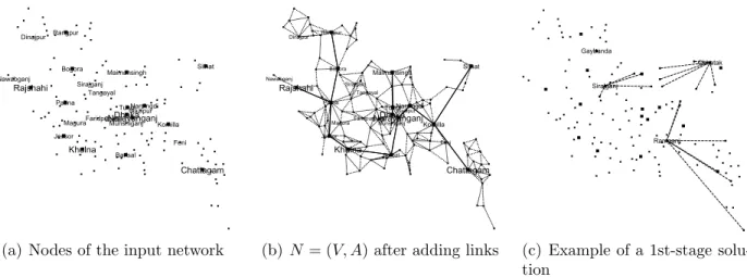
(a) Nodes of the input network (b) N= (V, A) after adding links (c) Example of a 1st-stage solu-tion
Figure 3: Construction process of Dis Instances and an example of a first-stage solution. Bangladesh
Instances.
is smaller than or equal toα/√n(αis an input parameter fixed to 1.6 in our computations).
Figure 3(a) shows the location of the 128 cities for theBangladesh group of instances,
Fig-ure 3(b) illustrates the embedded network N = (V, A) of the same group, and Figure 3(c)
shows an example of a first-stage solution.
With the information of each group, Bangladesh, Philippinesor ND-II, an instance of
the RRUFL is generated as follows:
(i) define R0 by randomly selecting t% of the cities, witht ∈ {25,50,75};
(ii) for k ∈K defineRk by randomly taking |R0| ×rand[0.4,0.6] cities from R0;
(iii) fork∈K defineJkby randomly taking (n−|Rk|)×rand[0.08,0.12] cities from 1, . . . , n
(J0 =∪
k∈KJk);
(iv) first-stage allocation costs c0ij are equal to the shortest path cost between i and j in
N = (V, A) using Euclidean distances duv, ∀{u, v} ∈A;
(v) for the second-stage allocation costs we consider random link interdiction, that is: let
Ik be a set of f× |A| ×rand[0.8,1.2] links randomly chosen from A. Then dkuv =duv,
for all {u, v} ∈ A\Ik, and dk
uv = 100×duv, for all {u, v} ∈ Ik, so ckij is equal to the
cost of the shortest path between i and j with edge costs given by dk. Reallocation
cost rijk is 1.5×dkij, fork ∈K;
(vi) first-stage set-up costs are given by f0
j =
P
i∈R0c0ij/|R0|, and second-stage set-up and
penalty costs are given by fjk = (1 +σ3)×fj0 and pkj = (1 +σ4)×fj0, for k∈K.
The remaining parameters are f ∈ {0,0.10,0.25,0.50}, σ3 = {0.00,1.00} and σ4 =
{0.10,1.0,4.0}. All possible parameter settings, in combination with k ∈ {25,50,75} imply
that there are 3×4×2×3×3 = 216 instances to be solved for each fixed value ofn within
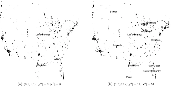
(a) (0.1,1.0),|y0|= 3,|x0|= 8 (b) (1.0,0.1),|y0|= 14,|x0|= 54
Figure 4: Solutions considering different combinations of (σ3, σ4) (InstancesUS,n= 500,ϕ= 0.001,ρ= 0.1
σ1= 0.5,σ2= 0.05 and|K|= 25)
4.2. Trans Instances: Solutions, Robustness and Recoverability
Influence of the Cost Structure The characteristics of arobust first-stage solution and the corresponding recovery actions depend not only on the scenario structure but also on the cost structure. If, for example, for a given instance the second-stage costs are very high with respect to the first-stage costs then the solutions of the RRUFL will tend to have more facilities and assignments defined in the first stage. Likewise, if the second-stage set-up costs
are much higher than the penalty costs (fk
j >> pkj), we would expect that more facilities
will be opened in the first-stage (and eventually more assignments) than if fjk ≤ pkj, where
the cost of setting-up a facility in the second stage is cheaper than the penalty for a facility placed at a non-available location.
In Figure 4 we show the later case by comparing two solutions of an instance of group US.
For the first one (Figure 4(a)), the penalties are≈81% more expensive than the second-stage
set-up costs, while for the second one (Figure 4(b)), the penalties are 45% cheaper. We can
see how changing the relation between fjk and pkj leads to very different solutions: while in
the first case 3 facilities are opened in the first stage and 8 customers are allocated to them, in the second case 14 facilities are opened in the first stage and 54 customers are allocated.
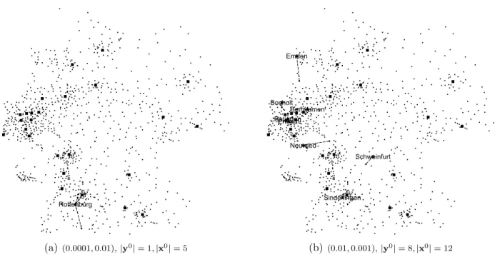
The relation between parameters ϕ ($ per unit of distance per inhabitant) and ρ ($ per
inhabitant), also influences the solution structure. Assume that we are given an instance with
ϕ < ρ (set-up costs are higher than the allocation costs) and another instance with ϕ > ρ
(allocation costs are higher than the set-up costs). We would expect that the solution of the second instance will be comprised by a larger first-stage component compared to the solution
of the first instance. Figure 5 depicts this by comparing the solution obtained forϕ= 0.0001
and ρ= 0.01 (Figure 5(a)) with the one obtained forϕ= 0.01 and ρ= 0.001 (Figure 5(b)).
(a) (0.0001,0.01),|y0|= 1,|x0|= 5 (b) (0.01,0.001),|y0|= 8,|x0|= 12
Figure 5: Solutions considering different combinations of (ϕ, ρ) (InstancesGer,n= 250,σ1= 0.5,σ2= 0.5
σ3= 0.1,σ4= 1.0 and|K|= 25)
while in the second case 8 facilities are installed and 12 allocations are established in the first stage. This effect is quite intuitive considering that the second stage costs are proportional to the first stage costs for these instances: it is better to open facilities in the same place
where the demand is located, i.e., in a subset of R0 ∩J0, in order to avoid high allocation
expenses (ϕ > ρ).
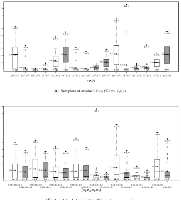
A more extensive analysis on the influence of the second-stage cost parameters (ϕ, ρ) and
(σ1, σ2, σ3, σ4) on the performance of the algorithm and on the the solutions characteristics
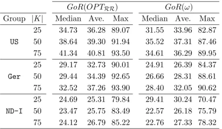
is now presented. In Figure 6(a) we show the box-plots of the attained gaps for all the
combinations of (ϕ, ρ) when solving Germany group with n = 250. Each box-plot contains
information about 48 instances. The maximum and attained gaps are marked with a bold circle and an asterisk, respectively, and the number of instances solved to optimality is
displayed under each box-plot. Recall that ϕis a factor expressed in $ per unit of distance
per unit of demand, and ρ is expressed in $ per inhabitant. We can observe the following:
(i) The problem becomes easier (more instances can be solved to optimality) when ϕ is
considerably smaller than ρ (103−105 times smaller), that is, for those instance where the
set-up costs are considerably higher than the operating costs (transportation). (ii) When
ρ < ϕ we have that the transportation costs are larger than the set-up costs; in these cases
the attained gaps are relatively small. (iii) The problems become harder when ϕρ ≥ 10−2.
These three behaviors can be explained by the fact that in the easier first two cases there is not as much symmetry in the cost structure between opening and transportation costs as in in the third case (where the opening and transportation costs are of the same magnitude).
In Figure 6(b) we show the box-plots of the attained gaps for the 16 combinations of
(σ1, σ2, σ3, σ4). Average and maximum gaps are marked with bold circles and asterisk as