VALID INEQUALITIES AND REFORMULATION
TECHNIQUES FOR MIXED INTEGER
NONLINEAR PROGRAMMING
by
Sina Modaresi
B.S., Sharif University of Technology, 2010
M.S., University of Pittsburgh, 2012
Submitted to the Graduate Faculty of
the Swanson School of Engineering in partial fulfillment
of the requirements for the degree of
Doctor of Philosophy
University of Pittsburgh
2015
UNIVERSITY OF PITTSBURGH
SWANSON SCHOOL OF ENGINEERING
This dissertation was presented
by
Sina Modaresi
It was defended on
November 12, 2015
and approved by
Jayant Rajgopal, Ph.D., Professor, Department of Industrial Engineering
Oleg A. Prokopyev, Ph.D., Associate Professor, Department of Industrial Engineering
Andrew J. Schaefer, Ph.D., Noah Harding Chair and Professor, Department of
Computational and Applied Mathematics, Rice University
Juan Pablo Vielma, Ph.D., Richard S. Leghorn Career Development Assistant Professor,
Sloan School of Management, Massachusetts Institute of Technology
Dissertation Director: Jayant Rajgopal, Ph.D., Professor, Department of Industrial
VALID INEQUALITIES AND REFORMULATION TECHNIQUES FOR MIXED INTEGER NONLINEAR PROGRAMMING
Sina Modaresi, PhD
University of Pittsburgh, 2015
One of the most important breakthroughs in the area of Mixed Integer Linear Programming (MILP) is the characterization of the convex hull of specially structured non-convex poly-hedral sets in order to develop valid inequalities or cutting planes. Development of strong valid inequalities such as Split cuts, Gomory Mixed Integer (GMI) cuts, and Mixed Integer Rounding (MIR) cuts has resulted in highly effective branch-and-cut algorithms. While such cuts are known to be equivalent, each of their characterizations provides different advantages and insights.
The study of cutting planes for Mixed Integer Nonlinear Programming (MINLP) is still much more limited than that for MILP, since characterizing cuts for MINLP requires the study of the convex hull of a non-convex and non-polyhedral set, which has proven to be significantly harder than the polyhedral case. However, there has been significant work on the computational use of cuts in MINLP. Furthermore, there has recently been a significant interest in extending the associated theoretical results from MILP to the realm of MINLP.
This dissertation is focused on the development of new cuts and extended formulations for Mixed Integer Nonlinear Programs. We study the generalization of split, k-branch split, and intersection cuts from Mixed Integer Linear Programming to the realm of Mixed Integer Nonlinear Programming. Constructing such cuts requires calculating the convex hull of the difference between a convex set and an open set with a simple geometric structure. We introduce two techniques to give precise characterizations of such convex hulls and use them to construct split, k-branch split, and intersection cuts for several classes of non-polyhedral
sets. We also study the relation between the introduced cuts and some known classes of cutting planes from MILP. Furthermore, we show how an aggregation technique can be easily extended to characterize the convex hull of sets defined by two quadratic or by a conic quadratic and a quadratic inequality. We also computationally evaluate the performance of the introduced cuts and extended formulations on two classes of MINLP problems.
Keywords: Mixed Integer Linear Programming, Mixed Integer Nonlinear Programming, Valid Inequality, Split Cut, K-branch Split Cut, Gomory Mixed Integer Cut, Mixed Integer Rounding Cut, Intersection Cut, Branch-and-Cut, Extended Formulation.
TABLE OF CONTENTS
PREFACE . . . x
1.0 INTRODUCTION . . . 1
2.0 NOTATION AND PRELIMINARIES. . . 4
3.0 INTERSECTION CUTS FOR NONLINEAR INTEGER PROGRAM-MING: CONVEXIFICATION TECHNIQUES FOR STRUCTURED SETS . . . 5
3.1 Notation, Known Results and Other Preliminaries . . . 7
3.2 Intersection Cuts through Interpolation . . . 11
3.2.1 Split Cuts for Epigraphical Sets . . . 11
3.2.1.1 Separable Functions . . . 14
3.2.1.2 Non-separable Positive Homogeneous Functions. . . 16
3.2.2 Split Cuts For Level Sets . . . 22
3.2.3 Non-trivial Extensions . . . 23
3.2.3.1 t-inclusive Split Cuts for Epigraphical Sets . . . 23
3.2.3.2 k-branch Split Cuts for Epigraphical Sets . . . 25
3.3 Intersection Cuts for Conic Quadratic Sets . . . 26
3.3.1 Split Cuts for Conic Quadratic Sets. . . 29
3.3.2 t-inclusive Split Cuts for Conic Quadratic Sets . . . 32
3.3.3 k-branch Split Cuts for Conic Quadratic Sets . . . 37
3.4 General Intersection Cuts through Aggregation . . . 38
3.4.1 Intersection Cuts for Epigraphs . . . 39
3.4.3 Intersection Cuts for Quadratic Sets . . . 41
3.5 Acknowledgments . . . 45
4.0 SPLIT CUTS AND EXTENDED FORMULATIONS FOR MIXED IN-TEGER CONIC QUADRATIC PROGRAMMING . . . 46
4.1 Notation and Previous Work . . . 47
4.2 Conic MIR and Linear Split Cuts . . . 50
4.3 Comparison between Cuts . . . 53
4.3.1 Containment Relations. . . 53
4.3.2 Bound Strength. . . 58
4.4 Acknowledgments . . . 60
5.0 CONVEX HULL OF TWO QUADRATIC OR A CONIC QUADRATIC AND A QUADRATIC INEQUALITY . . . 61
5.1 Notation, preliminaries, and existing convex hul results . . . 63
5.1.1 Preliminaries . . . 63
5.1.2 homogeneous quadratic sets . . . 65
5.1.3 Quadratic sets . . . 68
5.2 Conic quadratic characterization of convex hulls . . . 68
5.2.1 Conic quadratic representation of convex hulls . . . 69
5.2.2 Conic quadratic sets . . . 70
5.3 Conic quadratic characterization of closed convex hulls . . . 73
5.3.1 Homogeneous quadratic sets . . . 74
5.3.2 Conic quadratic sets . . . 74
5.3.3 Quadratic sets . . . 75
5.3.4 Verifying the topological condition . . . 76
5.3.5 Illustrative examples . . . 77
5.3.6 Comparison to the closed convex hull characterizations by Burer and Kılın¸c-Karzan . . . 83
6.0 COMPUTATIONAL EXPERIMENTS WITH CUTS AND EXTENDED FORMULATIONS . . . 88
6.0.8 Closest Vector Problem . . . 90
6.0.8.1 Test Instances . . . 92
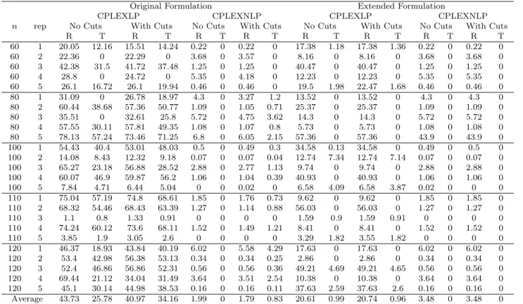
6.0.8.2 Results . . . 92
6.0.9 Mean-Variance Capital Budgeting (MVCB) . . . 95
6.0.9.1 Test Instances . . . 96
6.0.9.2 Results . . . 97
6.0.10 Concluding Remarks . . . 100
7.0 CONCLUSIONS . . . 102
LIST OF TABLES
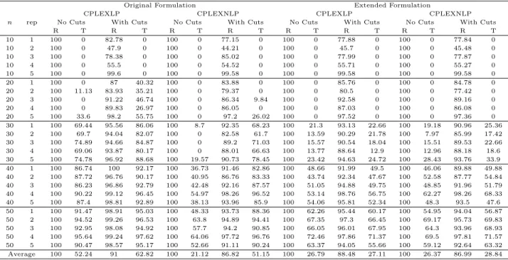
1 Gaps for CVP Instances . . . 92
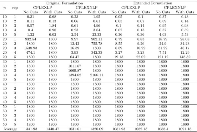
2 Solve Times for CVP Instances . . . 94
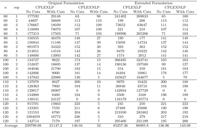
3 Node Counts for CVP Instances . . . 95
4 Gaps for MVCB Instances . . . 97
5 Solve Times for MVCB Instances . . . 98
6 Node Counts for MVCB Instances . . . 99
LIST OF FIGURES
1 Interpolation Technique for Univariate Functions.. . . 12
2 Nonlinear Interpolation for Non-separable Functions. . . 17
3 Friends Construction for Non-separable Positive Homogeneous Functions. . . 18
PREFACE
to my parents, Yousef and Maliheh
This work would not have been possible without the guidance of Dr. Juan Pablo Vielma, my mentor and advisor. I would like to express my deepest gratitude to him, first and fore-most, for his constant support, encouragement, professional attitude, constructive criticism, and most importantly, patience.
I would also like to thank the other members of my doctoral committee, Dr. Jayant Rajgopal, Dr. Oleg Prokopyev, and Dr. Andrew Schaefer for their valuable suggestions and comments.
Finally, I am forever indebted to my parents, Yousef and Maliheh, my brother, Sajad, and my sister, Zahra, for their endless love, inspiration, encouragement, and unconditional support.
1.0 INTRODUCTION
An important are of Mixed Integer Linear Programming (MILP) is the characterization of the convex hull of specially structured non-convex polyhedral sets to develop valid inequal-ities or cutting planes [10, 11, 30, 31, 32, 33, 38, 42, 62, 90]. Development of strong valid inequalities such as Split cuts [32], Gomory Mixed Integer (GMI) cuts [48, 49], and Mixed Integer Rounding (MIR) cuts [66, 74, 75, 93] has resulted in highly effective branch-and-cut algorithms [4, 22, 23, 55, 63]. While such cuts are known to be equivalent [39, 75], each of their characterizations provide different advantages and insights.
The study of cutting planes for Mixed Integer Nonlinear Programming (MINLP) is still much more limited than that for MILP, since characterizing cuts for MINLP requires the study of the convex hull of a non-convex and non-polyhedral set, which has proven to be significantly harder than the polyhedral case. However, there has been significant work on the computational use of cuts in MINLP [25, 28, 44, 59, 87]. Moreover, there has recently been a significant interest in extending the associated theoretical results from MILP to the realm of MINLP [18, 19, 35, 36, 37, 81]. In particular, for the case of Mixed Integer Conic Quadratic Programming (MICQP), there has been a recent surge of theoretical developments [6,8, 9, 14,15,16, 27, 57, 58, 73,71,72,70, 96, 91]. However, most of the known results in the area of MINLP are still limited to very specific sets [54,86, 88] or to approximations of semi-algebraic sets through Semidefinite Programming (SDP) [45, 61, 76,77, 78, 79, 80].
While the resulting cuts for MINLP are strong nonlinear inequalities, adding such non-linear cuts to the continuous relaxation of a MINLP could significantly increase its solution time. Hence there will likely be a strong trade-off between the strength provided by such cuts and their computational cost. It is then unclear if such nonlinear cuts can provide a significant computational advantage over linearization approaches such as those in [25, 59]
which do not require explicit cut formulas. However, even in such cases, the developed nonlinear cuts can provide valuable information about the performance of the linearization approaches. For instance, the linearization approaches can sometimes require a large num-ber of iterations to yield a bound improvement similar to that obtained by the associated nonlinear cut. Adding the nonlinear cut provides a simple way to evaluate if the lack of bound improvement is due to lack of strength of the cut or lack of convergence of the lin-earization approach. Similarly, the availability of explicit formulas of split cuts for quadratic sets proven extremely useful to evaluate the strength of a cutting plane approach based on extended formulations in [71].
This dissertation is focused on the development of new cuts and extended formulations for Mixed Integer Nonlinear Programs. We study the generalization of split, k-branch split, and intersection cuts from Mixed Integer Linear Programming to the realm of Mixed Integer Nonlinear Programming. Constructing such cuts requires calculating the convex hull of the difference between a convex set and an open set with a simple geometric structure. We introduce two techniques to give precise characterizations of such convex hulls and use them to construct split, k-branch split, and intersection cuts for several classes of non-polyhedral sets. We also study the relation between the introduced cuts and some known classes of cutting planes from MILP. Furthermore, we show how an aggregation technique can be easily extended to characterize the convex hull of sets defined by two quadratic or by a conic quadratic and a quadratic inequality. We also computationally evaluate the performance of the introduced cuts and extended formulations on two classes of MINLP problems.
The remainder of this dissertation is organized as follows. In Chapter 3 we study the generalization of split, k-branch split, and intersection cuts from MILP to MINLP. We pro-pose two simple techniques to derive general intersection cuts for several classes of MINLP problems with specific structures. In particular, we give simple formulas for split cuts for essentially all convex sets described by a single conic quadratic inequality. We also give simple formulas for k-branch split cuts and some general intersection cuts for a wide variety of convex quadratic sets.
In Chapter4we study split cuts and extended formulations for MICQP. In particular, we study the relation between Conic MIR (CMIR) cuts introduced by Atamt¨urk and Narayanan
[9] and nonlinear split cuts for a class of MICQP problems. We also study an extended for-mulation for such a class of MICQP and illustrate how the power of an extended forfor-mulation can improve the strength of a cutting plane procedure in MINLP.
In Chapter 5 we consider an aggregation technique introduced by Yıldıran [94] to study the convex hull of regions defined by two quadratic or by a conic quadratic and a quadratic inequality. Yıldıran [94] shows how to characterize the convex hull of sets defined by two quadratics using Linear Matrix Inequalities (LMI). We show how this aggregation technique can be easily extended to yield valid conic quadratic inequalities for the convex hull of sets defined by two quadratic or by a conic quadratic and a quadratic inequality. We also show that in many cases under additional assumptions, these valid inequalities characterize the convex hull exactly.
In Chapter 6 we computationally evaluate the performance of the introduced linear and nonlinear cuts and extended formulations on two classes of MINLP problems (Closest Vector Problem and Mean-variance Capital Budgeting). We compare the strength of the nonlinear cuts added to the original formulations versus the linear cuts added to an extended formulation.
Finally, Chapter 7concludes the discussion summarizing the contributions of this disser-tation.
2.0 NOTATION AND PRELIMINARIES
We use the following notation throughout the dissertation. Letei ∈
Rn be thei-th unit vec-tor, 0n ∈Rn be the zero vector, I ∈ Rn×n be the identity matrix wheren is an appropriate
dimension that we omit if evident from the context, andSn denote symmetric matrices with n rows and columns. For a ∈R we let (a)+ := max{0, a} and bac := max{k ∈Z : k ≤a}. We also let kxk2 := pPni=1x2i denote the Euclidean norm of x ∈ Rn and |x| ∈
Rn be the vector whose components are the absolute value of the components of x ∈Rn. In addition,
we let kxkp := (Pni=1|xi|p)1/p denote the p-norm of a given vector x ∈Rn and for a vector v ∈Rn, we let the projection onto its span beP
v := vv
T
kvk2 2
and onto its orthogonal complement be Pv⊥ :=I − vvT kvk2 2. We also let {πi} k i=1 ⊆ R n\ {0
n} be an arbitrary set of vectors, and not
necessarily a sequence of vectors. For a matrixP, we letπ(P) denote the number of negative eigenvalues of P and null(P) denote its null space. For a set S ⊆ Rn, we let int (S) be its
interior, bd (S) be its boundary, conv (S) be its convex hull, conv (S) be the closure of its con-vex hull, aff (S) be its affine hull, lin (S) :={d∈Rn : x+λd∈S for all x∈S and λ∈
R} be its lineality space, and S∞ be its recession cone. For a function G : Rn → R we let epi (G) := {(x, t)∈Rn+1 : G(x)≤t} be its epigraph, gr (G) := {(x, t)∈
Rn+1 : G(x) = t} be its graph, and hyp (G) := {(x, t)∈Rn+1 : G(x)≥t} be its hypograph. In addition,
we let the second-order cone (a.k.a. Lorentz cone) be the epigraph of the Euclidean norm defined as {(x, t)∈Rn+1 : kxk
3.0 INTERSECTION CUTS FOR NONLINEAR INTEGER PROGRAMMING: CONVEXIFICATION TECHNIQUES FOR
STRUCTURED SETS
One of the most important breakthroughs in the area of Mixed Integer Linear Programming (MILP) is the development of strong valid inequalities or cutting planes such as split and intersection cuts. However, the study of cuts for Mixed Integer Nonlinear Programming (MINLP) is still much more limited than that for MILP. Most of the known results in this area are limited to very specific sets [54, 86, 88] or to approximations of semi-algebraic sets through Semidefinite Programming (SDP) [45, 61, 76, 77, 78, 79, 80]. While some precise SDP representations of the convex hulls of semi-algebraic sets exist [50, 51, 52, 85], these require the use of auxiliary variables. Such higher dimensional, extended, or lifted represen-tations are extremely powerful. However, there are theoretical and computational reasons to want representations in the original space and/or in the same class as the original set (e.g. representations that do not jump from quadratic basic semi-algebraic to SDP). We refer to characterizations that satisfy both these requirements as projected and class preserving. Projected and class preserving are in general incompatible (e.g. the convex hull of the basic semi-algebraic set{x∈R2 : (x2
1−x2)x1 ≥0, x2 ≥0}has no projected basic semi-algebraic
representation, but has a lifted basic semi-algebraic representation [24]). Furthermore, even giving an algebraic characterization of the boundary of the convex hull of a variety [82, 83] or giving a projected SDP representation of the convex hull of certain varieties and quadratic semi-algebraic sets [84, 94, 95] requires very complex techniques from algebraic geometry. All such issues make extending MILP cutting planes to the MINLP setting extremely chal-lenging. To alleviate such challenges, in this chapter we concentrate on the extension of split, k-branch split, and other intersection cuts to the MINLP setting [10,32, 38, 48,49, 62].
Split, k-branch split, and intersection cuts for MILP can all be obtained by taking the convex hull of the difference between a convex set and a set with a simple geometric structure. This characterization allows for a straightforward extension of the cuts to the MINLP setting. However, this conceptual extension does not provide a practical construction procedure for the cuts. For this reason, we follow the approach of the simple, but extremely powerful Mixed Integer Rounding (MIR) cut [66, 74, 75, 93]. The MIR procedure can be used to generate every split cut for a MILP and, together with the closely related Gomory Mixed Integer (GMI) cut procedure [48, 49], yields the most effective cutting plane approach for general MILP [22, 23]. In particular, one version of the MIR procedure shows that every split cut can be constructed through a simple two step procedure. The first step is the construction of a canonical cut known as thesimple orbasic MIR. This cut is obtained by taking the convex hull of the difference between two simple convex sets in R2, both of which are described by
two linear inequalities. The second step simply uses linear transformations to obtain all split cuts from the basic MIR. In this chapter we show that a similar approach can be used to construct a wide range of intersection cuts. More specifically, we show how two very simple techniques can be used to construct projected class preserving characterizations of the convex hull of difference between certain canonical sets. The techniques we consider are only tailored to the geometric structure of these canonical sets and do not require the sets to have any additional algebraic properties (e.g. being quadratic, basic semi-algebraic, etc.). Thanks to this, the resulting characterizations are quite general, but give simple closed form expressions. While the canonical sets are somewhat specific, we can also use affine transformations to obtain more general cuts. In particular, these techniques can be used to construct split cuts for essentially all convex sets described by a single conic quadratic inequality, and to extend k-branch split and general intersection cuts to a wide variety of quadratic sets of interest to trust region and lattice problems. In both cases, the only algebraic property of the quadratic sets needed for the construction is the symmetry of the Euclidean norm. This suggests that the techniques could be useful to construct cuts for additional classes of sets by only exploiting similar basic properties.
Constructing such cuts requires calculating the convex hull of the difference between a convex set and an open set with a simple geometric structure. We introduce two techniques
to give precise characterizations of such convex hulls and use them to construct split, k-branch split, and intersection cuts for several classes of non-polyhedral sets. In particular, we give simple formulas for split cuts for essentially all convex sets described by a single conic quadratic inequality. We also give simple formulas for k-branch split cuts and some general intersection cuts for a wide variety of convex quadratic sets.
The rest of this chapter is organized as follows. We begin with Section 3.1 where we introduce some notation and review some known results. Section 3.2 then introduces an interpolation technique that can be used to construct split and k-branch split cuts for many classes of sets. Then, in Section 3.3 we use the interpolation technique to characterize intersection cuts for conic quadratic sets. Finally, Section 3.4 introduces an aggregation technique that can be used to construct a wide array of general intersection cuts. In both Sections3.2 and 3.4, we first present the basic principles behind the techniques in a simple, but abstract setting, and then utilize them to construct more specific cuts to illustrate their power and limitations.
3.1 NOTATION, KNOWN RESULTS AND OTHER PRELIMINARIES
In addition to the notation introduced in Chapter 2, we use the following notation and definitions in this chapter.
Definition 1 (Intersection, Split, k-branch Split, and t-inclusive Split Cuts). Let B ⊆Rn be
a closed convex set that we refer to as the base set, F ⊆Rnbe a closed set that we refer to as
the forbidden set, andg :Rn→Rbe an arbitrary function. We say inequality g(x)≤0is an
intersection cut for B and F if conv (B\int (F))⊆ {x∈Rn : g(x)≤0} and g is convex.
We let a split be a set of the form x∈Rn : πTx∈[π
0, π1] for some π ∈ Rn\ {0n}
and π0, π1 ∈ R such that π0 < π1. If F is a split, we say that the associated intersection cut is a split cut. Besides, if F is a split with π =ei for some i∈ [n], we refer to F as an
We let a k-branch split be a set of the form Ski=1x∈Rn : πi
0 ≤πiTx≤πi1 for some {πi}
k
i=1 ⊆Rn\ {0n}, πi0, πi1 ∈R such that πi0 < π1i for alli∈[k]. If F is a k-branch split, we say that the associated intersection cut is a k-branch split cut.
When considering epigraphical sets of the form B ={(x, t)∈Rn+1 : G(x)≤t} for some closed convex function G(x), we often assume that F is a cylinder whose axis lies along t
(i.e., F is of the form S×R for some S ⊆Rn). For instance, if F is a split, we have F =
(x, t)∈Rn+1 : πTx∈[π
0, π1] . However, in some cases, we consider a split that includes
t and we refer to such a split as a t-inclusive split. More specifically, we let a t-inclusive split be a set of the form (x, t)∈Rn+1 : πTx+ ˆπt∈[π
0, π1] for some (π,π)ˆ ∈Rn+1 such
that ˆπ 6= 01, and π
0, π1 ∈ R such that π0 < π1. If F is a t-inclusive split, we say that the associated intersection cut is a t-inclusive split cut.
We mostly restrict to the cases in which conv (B\int (F)) is closed, so for notational convenience, we let B := conv (B\int (F)) whenF is evident from the context.
We note that the term intersection cut was introduced by Balas [10] for the case in which B is a translated simplicial cone, F is the euclidean ball or a cylinder of a lower dimensional euclidean ball, and the unique vertex of B is in int (F). In this setting, we have that conv (B\int (F)) is closed and can be described by adding a single linear inequality to B. Furthermore, this single linear inequality has a simple formula dependent on the inter-sections of the extreme rays of B with F. While we do not always have such intersection formulas for other classes of sets, we continue to use the term intersection cut in the more general setting and avoid any additional qualifiers for simplicity. In particular, we do not use the term generalized intersection cut as it has already been used for the case of polyhedral B and F and in conjunction with an improved cut generation procedure for MILP [12]. The term split cut was introduced by Cook, Kannan and Schrijver [32], and their original definition directly generalizes to non-polyhedral sets as in Definition 1. The term k-branch split cut was introduced by Li and Richard [62]; 2-branch split cuts are also called cross cuts in Dash, Dey and G¨unl¨uk [38]. These definitions also directly generalize to non-polyhedral sets as in Definition 1.
1We allowπ= 0
The interest of intersection cuts for MILP and MINLP arises from the fact that if int(F)∩
(Zp×
Rq) = ∅, an intersection cut for B and F is valid for conv (B∩(Zp×Rq)). Hence, intersection cuts can be used to strengthen the continuous relaxation of MILP and MINLP problems.
Intersection cuts are particularly attractive in the MILP setting, since they can be quite strong and can easily be constructed. They were extensively studied when they were first proposed in the 1970s [10, 48, 49] and have recently received renewed interest [31, 42]. Part of the relative simplicity and effectiveness of intersection cuts for MILP stems from two basic facts. The first one is that in the MILP setting, B is a polyhedron (i.e., the continuous relaxation of a MILP is an LP). The second one is the fact that every convex setF such that int(F)∩Zn=∅(usually denoted a lattice free convex set) and that is maximal with respect
to inclusion for this property is also a polyhedron [64]. Restricting both B and F to be (convex) polyhedra give intersection cuts for MILP several useful properties. For instance, if B and F are polyhedra, then conv (B \int (F)) is a polyhedron [42]. Hence, in the MILP setting, we can restrict our attention to linear intersection cuts. In particular, ifF is a split and B is a polyhedron, then all linear intersection cuts for B and F can be constructed from simplicial relaxations of B and hence have simple formulas [5, 40, 89]. As discussed in the introduction, GMI cuts [48, 49] and MIR cuts [66, 74, 75, 93] are two versions of these formulas. For more information on the ongoing efforts to duplicate this effectiveness for other lattice free polyhedra, we refer the reader to [31,42]. In this context, we note that conv (B\int (F)) can fail to be closed even if B and F are polyhedra and F is not a split (e.g. consider B = {x∈R2 : x
2 ≥0} and F ={x∈R2 : x2 ≤1, x1+x2 ≤1}). However,
conv (B\int (F)) is closed in the polyhedral case if F is convex and full-dimensional and the recession cone of F is a linear subspace [7].
In the MINLP setting, there has been significant work on the computational use of linear split cuts [25, 28, 87, 44, 59]. From the theoretical side, we know that if F is a split, then conv (B\int (F)) is closed even if B is not polyhedral [37]. With respect to formulas for intersection cuts, there has been some progress in the description of split cuts for quadratic sets in [8, 9,37, 14]. Dadush et al. [37] show that, if B is an ellipsoid and F is a split, then conv (B\int (F)) can be described by intersectingB with either a linear half space, an affine
transformation of the second-order cone, or an ellipsoidal cylinder. In addition, they give simple closed form expressions for all these linear and nonlinear split cuts. Independently, [14] studies split cuts for more general quadratic sets, but only for splits in which{x∈B : πTx=
π0}and{x∈B : πTx=π1}are bounded. They give a procedure to find the associated split
cuts, but do not give closed form expressions for them. Finally, [8, 9] give a simple formula for an elementary split cut for the standard three dimensional second-order cone. While [14] develops a procedure to construct split cuts through a detailed algebraic analysis of quadratic constraints developed in [15], [8, 9,37] give formulas for split cuts through simple geometric arguments. As we have recently shown at the MIP 2012 Workshop, these geometric techniques can be extended to additional quadratic and basic semi-algebraic sets [69]. In this paper we show that the principles behind these geometric arguments can be abstracted from the semi-algebraic setting to develop split and k-branch split cut formulas for a wider class of specially structured convex sets. This abstraction greatly simplifies the proofs and can be used to construct split cuts for essentially all convex sets described by a single conic quadratic inequality through simple linear algebra arguments. In addition to studying split and k-branch split cuts, we show how a commonly used aggregation technique can be used to develop formulas for general nonlinear intersection cuts for the case in which B and F are both non-polyhedral, but share a common structure. While a non-polyhedral F is not necessary in the MINLP settings (it still should be sufficient to consider maximal lattice free convex sets, which are polyhedral), they could still provide an advantage and are important in other settings such as trust region problems [18, 19, 79] and lattice problems [26, 71]. We finally note that similar results for the quadratic case have recently been independently developed in [6]. We discuss the relation between the results in [6] and our work at the end of Section3.3.2.
To describe our approach, we use the following additional definition.
Definition 2. Let B ⊆Rn be a closed convex set, F ⊆
Rn be a closed set, and g :Rn →R
be an arbitrary function. We say inequality g(x)≤0 is a:
• valid cut if B ⊆ {x∈Rn : g(x)≤0},
• sufficient cut, if {x∈B : g(x)≤0} ⊆B.
Binding valid cuts correspond to valid cuts that cannot be improved by translations, and sufficient cuts are those that are violated by any point of B outside B. We can show that a convex cut that is sufficient and valid is enough to describe B together with the original constraints defining B. Our approach to generating such cuts will be to construct cuts that are binding and valid by design, and that have simple structures from which sufficiency can easily be proven.
3.2 INTERSECTION CUTS THROUGH INTERPOLATION
In this section we consider the case in which the base set is either the epigraph, lower level set, or a section of the epigraph of a convex function and the forbidden set corresponds to a split, t-inclusive split, or a k-branch split. Our cut construction approach is based on a simple interpolation technique that can be more naturally explained for splits and epigraphs of specially structured functions. For this reason, we begin with such a case and then consider special cases of non-epigraphical sets and discuss the limits of the interpolation technique. While the structures for which the technique yields simple formulas are quite specific, we can consider broader classes by considering affine transformations. In Section 3.3 we illustrate the power of this approach by showing how the interpolation technique yields formulas for intersection cuts for convex quadratic sets.
3.2.1 Split Cuts for Epigraphical Sets
LetG:R→R be a closed convex function and letF be an elementary split associated with π =e1. Then epi(G) = epi(G)∩epi(J) for
J(z) = G(π1)−G(π0) π1−π0
z+π1G(π0)−π0G(π1) π1−π0
. (3.1)
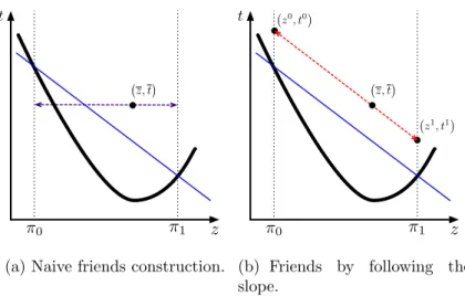
This is illustrated in Figure1, where the graph ofGis given by the thick black curve and the graph of J is depicted by the thin blue line. Indeed, since J is a linear function and hence
z, t
(a) Naive friends construction.
z, t
z1, t1 z0, t0
(b) Friends by following the slope.
Figure 1: Interpolation Technique for Univariate Functions.
epi(G)∩epi(J) convex, it is enough to show that J(z)≤t is a valid and sufficient cut. We can check thatJ(z)≤t is a binding valid cut becauseJ is the (affine) linear interpolation of G through z =π0 and z =π1. Convexity of G then implies that this interpolation is below
G for z /∈(π0, π1).
To show that the cut is sufficient, we need to show that any point z, t ∈ epi(G) that satisfies the cut is in epi(G). To achieve this, we can find two points (z0, t0) and (z1, t1) in
epi(G) such that z0 ≤ π0, z1 ≥ π1, and z, t
∈ conv ({(z0, t0),(z1, t1)}). Following [41], we will denote these points the friends of z, t. One naive way to construct the friends is to wiggle z, t by decreasing and increasing z until it reaches π0 and π1, respectively.
However, as illustrated in Figure 1(a), this can result in one of the friends falling outside epi(G). Fortunately, as illustrated in Figure 1(b), we can always wiggle by following the slope of the cut J to assure that the friends are in epi(J). Correctness (i.e., containment of the friends in epi(G)) then follows by noting that J(z) = G(z) at z = π0 and z = π1,
since J(z)≤ t is a binding valid cut. This two-stage procedure of binding validity through interpolation and sufficiency through friends can be formalized for general closed convex sets as follows.
Proposition 1. Let B ⊆ Rn be a closed convex set and F ⊆
Rn be closed. If C ⊆ Rn is a
closed convex set such that
B∩bd (F) = C∩bd (F) (3.2a)
B\int (F) ⊆ C\int (F), (3.2b)
and if
for all x¯∈C∩int (F)there exists a finite set Γ⊆C∩bd (F) such that x¯∈conv (Γ), (3.3)
then
B =B∩C. (3.4)
Proof. We have that
B\int (F)⊆B∩C ⊆B, (3.5)
where the first containment comes from (3.2b) and the last from (3.3) and (3.2a). The result follows by taking convex hull in (3.5) and noting that B∩C is convex because both B and C are convex.
Note that if F is a split, we can always consider Γ containing exactly two points (e.g Figure1and Propositions2and4), while larger sets Γ might be necessary for other forbidden sets (e.g. Proposition7). Our general approach to use Proposition1is to construct a convex function that yields binding valid cuts (i.e., satisfies (3.2)) and to use its specific geometric structure to construct friends for sufficiency. We now consider two structures in which the appropriate interpolation can easily be constructed once we identify the interpolation’s general form. The geometric structures of the resulting cuts yield two friends construction techniques. The first technique generalizes the univariate argument in Figure1(b) by noting that following the slope of J is equivalent to moving in lin (epi(J)). The second technique constructs the friends by moving in a ray contained in an appropriately constructed cone. These techniques are described in detail in Sections 3.2.1.1and 3.2.1.2respectively.
3.2.1.1 Separable Functions Let G be a separable function of the form G(z, y) = f(z) +g(y) with f : R → R and g : Rp →
R closed convex functions, and let F be an elementary split associated with π = e1. Analogous to (3.1), we can simply interpolate G
parametrically on y to obtain J(z, y) = G(π1, y)−G(π0, y) π1−π0 z+ π1G(π0, y)−π0G(π1, y) π1−π0 . (3.6)
In this case, the interpolation simplifies toJ(z, y) = f(π1)−f(π0)
π1−π0 z+
π1f(π0)−π0f(π1)
π1−π0 +g(y), which
is convex on (z, y) and linear onz. Our original univariate argument follows through directly and we get epi (G) = epi (G)∩epi (J). To illustrate this, consider G :R×R→R given by G(z, y) =z2 +y2 and let F be the elementary split associated with π =e1, π0 =−10, and
π1 = 1. Constructing a parametric linear interpolation as in (3.6) yields
J(z, y) = 1−100
11 z+
(100 +y2) + 10 (1 +y2)
11 =−9z+ 10 +y
2.
Function J is convex on (z, y), linear on z, and satisfies the conditions of Proposition1. We can thus conclude that it yields the associated split cut. In contrast, if we consider the non-elementary split π = (1,1)T with the previous choices of π0 and π1 on the same
function G, we need to proceed with more care. In particular, the parametric interpolation (3.6) cannot be directly applied since the disjunction affects both z and y. However, we can construct the split cut by exploiting the fact that Gcan be represented as
G(z, y) = (z+y) 2 2 + (z−y)2 2 = πT(z, y)2 2 + hT(z, y)2 2 , (3.7)
where h = (1,−1)T is orthogonal to π. If we let ˜z = πT(z, y), ˜y = hT(z, y), ˜π = (1,0),
˜
π0 = −10, ˜π1 = 1, and ˜G(˜z,y) = ˜˜ z2/2 + ˜y2/2, we revert to the elementary case where we
can apply the parametric interpolation (3.6) to obtain the split cut
˜ J(˜z,y) =˜ ˜ G(˜π1,y)˜ −G˜( ˜π0,y)˜ ˜ π1−˜π0 ˜ z+π˜1 ˜ G(˜π0,y)˜ −π˜0G˜(˜π1,y)˜ ˜ π1−π˜0 = −9˜z+ 10 + ˜y 2 2 . (3.8)
We can then recover the split cut in the original (z, y) space by replacing the definitions of ˜
z and ˜y. The same procedure can be used for any separable function that is of, or can be converted to, the formG(x) =f(πTx) +g(P⊥
π x) whereg :Rn →Rand f :R→Rare closed
To formally prove this, we first show how the friends construction procedure of Fig-ure 1(b) can be extended to a general closed convex set C by considering properties of lin (C).
Proposition 2. Let F ⊆ Rn be a split and C ⊆
Rn be a closed convex set. If there exists u∈lin (C) such that πTu6= 0, then condition (3.3) in Proposition 1 is satisfied.
Proof. Let ¯x ∈ C such that πTx¯ ∈ (π
0, π1) and u ∈ lin (C) such that πTu 6= 0. Also let
xi := ¯x+λ
iu for i ∈ {0,1}, where λi = πi−π
T¯x
πTu , and let β ∈ (0,1) be such that πTx¯ =
βπ0 + (1−β)π1. Because u ∈ lin (C) and since πTxi = πi, we have xi ∈ C∩bd (F) for
i∈ {0,1}. The result then follows by noting that ¯x=βx0+ (1−β)x1.
Using Propositions 1and 2 we obtain the following split cut formula for separable func-tions.
Proposition 3. Let F be a split, g :Rn→
R and f :R→R be closed convex functions,
Sg,f := (x, t)∈Rn+1 :g(P⊥ π x) +f(π Tx)≤t , a= f(π1)−f(π0) π1−π0 , and b= π1f(π0)−π0f(π1) π1−π0 . Then Sg,f =Sg,f ∩C, where C =(x, t)∈Rn+1 : g(P⊥ π x) +aπTx+b ≤t .
Proof. Interpolation condition (3.2) holds by the definition of a and b and convexity of f. Friends condition (3.3) follows from Proposition 2 by noting that u= π, akπk22 ∈ lin (C) and (π,0)T u6= 0. The result then follows from Proposition 1.
3.2.1.2 Non-separable Positive Homogeneous Functions Proposition1can also be used to construct cuts for some non-separable functions, but as illustrated in the following example, we need slightly more complicated interpolations. Consider G:R×R →R given byG(z, y) = pz2+y2 and let F be the elementary split associated with π=e1, π
0 =−10,
and π1 = 1. Constructing a parametric linear interpolation as in (3.6) yields
JL(z, y) =
10p1 +y2+p100 +y2+zp1 +y2−p100 +y2
11 . (3.9)
The associated cut is certainly valid, binding, and sufficient for epi (G) (we can always find friends by wiggling z toward π0 and π1, and using t to correct by following the slope of JL
for fixed y). However, while J is linear with respect to z, it is not convex with respect to y. We hence cannot use Proposition 1for this interpolation. Fortunately, we can construct an alternative interpolation given by
JC(z, y) = s 20−9z 11 2 +y2 (3.10)
that is convex on (z, y). This function is not linear on z for fixed y, but we can still show it satisfies the interpolation condition (3.2) by noting that 2011−9z2 ≤ z2 for any
z /∈ (π0, π1) and that equality holds for z ∈ {π0, π1}. This is illustrated in Figure 2 for
y=−4 where the graphs ofG, JC, and JL are given by the thick black curve, the thin blue
curve, and the dash-dotted green line, respectively. The figure shows that JC(z, y) ≤ t is
a nonlinear binding valid cut, but is strictly weaker than JL(z, y) ≤ t. While JC yields a
weaker cut thanJL,JC is in fact the strongestconvex function that satisfies the interpolation
condition (3.2) and we can show that epi(G) = epi(G)∩epi(JC). However, for the point
z, y, t ∈ epi (JC)∩int (F) with y = −4 depicted in Figure 2, the friends construction
cannot be done by wiggling in a direction that leaves y fixed to −4. In other words, there are points in ˆH :={(z, y, t)∈R3 : y=−4}that do not have friends in ˆH. We can construct
friends by wiggling in a direction that does change y, but since lin(epi(JC)) = {0}, such a
direction cannot be directly obtained from Proposition 2. Fortunately, the general idea of Proposition 2 can be adapted to obtain a variant that directly reveals an appropriate direction.
z, y, t
Figure 2: Nonlinear Interpolation for Non-separable Functions.
The variant of Proposition 2 that we need, exploits a different geometric characteristic of epi (JC) through the generalization of a technique used in [8, 9]. The required geometric
characteristic is given by the following definition.
Definition 3. Let C ⊆ Rn be a closed convex set. We say C is a translated cone or conic
setif there exists x∗ ∈C such that C−x∗ is a convex cone. We refer to suchx∗ as an apex
of C, noting that it is not necessarily unique (e.g. a half space is a conic set whose apex is not unique).
One can check that epi (JC) is a conic set with the unique apex (z∗, y∗, t∗) = (20/9,0,0).
Hence, because (¯z, y,¯t)∈epi (JC), we have that the ray
R :={(z∗, y∗, t∗) +α((¯z, y,¯t)−(z∗, y∗, t∗)) : α≥0} ⊆epi (JC). (3.11)
Furthermore, becausez∗ > π1 and ¯z∈(π0, π1), there existsαi >0 such thatz∗+αi(¯z−z∗) =
πi for each i∈ {0,1}. Therefore the friends of (¯z, y,¯t) are given by (zi, yi, ti) := (z∗, y∗, t∗) +
αi((¯z, y,¯t)−(z∗, y∗, t∗)) for i∈ {0,1}.
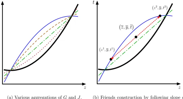
Figure 3 illustrates the ray-based friends construction for (¯z, y,¯t) with y = −4. Fig-ure 3(a) shows the construction in the (z, y, t) space, while Figure 3(b) shows the section
0 10 -10 -10 -5 0 5 z -10 0 10 y 0 5 10 15 t
(a) Construction in the (z, y, t) space.
z, y, t z0, y0, t0
z1, y1, t1
(b) Construction in the hyperplane ˜H.
Figure 3: Friends Construction for Non-separable Positive Homogeneous Functions.
obtained by intersecting Figure 3(a) with the hyperplane ˜H := aff (R∪ {(0,0,1)}), for the ray R given in (3.11). The intersection of ˜H with the bounding box is depicted by the dash-dotted line in Figure 3(a). The graph of G is given by a black wire-frame in Figure 3(a), while the intersection of this graph with ˜H is given by the thick black curve in both figures. Meanwhile, the graph of JC is depicted by the blue shaded region in Figure 3(a) and by a
thin blue curve in Figure 3(b). The figures also depict (zi, yi, ti) fori∈ {0,1} and (¯z, y,¯t) as black dots and (z∗, y∗, t∗) as a red box. In addition, the intersection of z =πi for i∈ {0,1}
with the epigraphs of bothGand JC are depicted in Figure 3(a)by the gray shaded regions.
The intersection of z =πi fori∈ {0,1}with ˜H are depicted in both figures by dotted lines.
Finally, ray R is depicted in both figures as a red dashed arrow. Note that ˜H is tilted in the (z, y) space precisely to contain (z∗, y∗, t∗) and (¯z, y,t). Noting that¯ y∗ 6= y we have that, unlike ˆH, ˜H allows the variation of y. Furthermore, while (¯z, y,t)¯ ∈Hˆ ∩H˜ might not have friends in ˆH, Figure 3 shows that it does have friends in ˜H. Similarly to Proposition2, the above construction can be extended to general convex sets as follows.
Proposition 4. Let F ⊆ Rn be a split. If C ⊆
Rn is a conic set with apex x∗ ∈ Rn such
that πTx∗ ∈/(π
Proof. Let ¯x ∈ C such that πTx¯∈ (π
0, π1). Note that since x∗ is the apex of C, all points
on the rayR :={x∗+α(¯x−x∗) :α∈R+} belong toC. Let the intersections ofR with the
hyperplanes πTx = π
0 and πTx = π1 be x0 and x1, respectively. Such points are obtained
fromRby settingαi = πi−π
Tx∗
πTx¯−πTx∗, fori∈ {0,1}. We havexi ∈C∩bd (F) fori∈ {0,1}, since πTxi = π
i and R ⊆ C. Note that ¯x is obtained from R by setting α = 1. If α0 < 1 < α1
or α1 < 1 < α0, then there exists β ∈ (0,1) such that ¯x = βx0 + (1−β)x1. Seeing that
πTx¯∈(π0, π1) and πTx∗ ∈/ (π0, π1), one can check α0 <1< α1 orα1 <1< α0.
Note that Propositions2and4ask for very different requirements onC. In Proposition2, we only need to have a direction u ∈ lin (C) such that πTu 6= 0. In such a case, C always
defines a non-pointed region (i.e., C contains a line). On the other hand, as illustrated by (3.10), the sets C for which Proposition 4 is applicable are usually pointed (i.e. C has at least one extreme point). However, pointedness is not a requirement in Proposition 4
(e.g. half-spaces are conic sets). The real price of Proposition 4 over Proposition 2 is requiring C to be conic, which is a much more global requirement than asking for the lineality space of C to contain a non-orthogonal direction toπ. However, both propositions are needed to construct split cuts for positive homogeneous functions. To see this, consider the same functionG(z, y) =pz2+y2 for which (3.10) yields a split cut, but instead consider
the split z ∈ [−1,1]. For this case, we can check that epi(G) = epi(G) ∩ epi(JD) for
JD(z, y) =
p
1 +y2, which does not have a conic epigraph. However, (1,0,0)∈lin(epi(J
C))
and hence Proposition 2 is applicable. This dichotomy between a non-pointed and a conic (and potentially pointed) cut will be a common occurrence that we highlight further when characterizing intersection cuts for conic quadratic sets in Section 3.3.
While Propositions 2 and 4 can be used to prove sufficiency of the split cuts for pos-itive homogeneous functions, such cuts first have to be constructed with an appropriate interpolation technique. Fortunately, both interpolations of G(z, y) =pz2+y2 (conic and
non-pointed) can be generalized to functions based onp-norms by using the following simple lemma.
Lemma 1. Let p ∈ N, π0, π1 ∈ R such that π0 < π1, l ∈ R, a = (
|l|p+|π1|p)1/p−(|l|p+|π0|p)1/p
π1−π0 ,
and b = π1(|l|p+|π0|p)1/p−π0(|l|p+|π1|p)1/p
• If s∈ {π0, π1}, then |as+b|p =|s|p+|l|p and • if s /∈(π0, π1), then |as+b|
p
≤ |s|p+|l|p.
Proof. We show the equivalent version of the lemma given by
1. If s∈ {π0, π1}, then |as+b|= (|s|p+|l|p)1/p and
2. if s /∈(π0, π1), then |as+b| ≤(|s|
p
+|l|p)1/p.
Let f(s) := as+b and g(s) := (|s|p +|l|p)1/p. By definition of a and b we have that
f(πi) = g(πi) for i∈ {0,1}. Indeed, f(s) is the (affine) linear interpolation of g(s) through
z = π0 and z = π1. Convexity of g(s) then implies f(s) ≤ g(s) for all s /∈ (π0, π1).
If |π0| = |π1|, then |as+b| = f(s) and the result follows directly. If |π0| 6= |π1|, one
can check that |as+b| = f(s) for s ∈ [π0, π1] and hence (1) holds. For (2) it suffices
to show that −as −b ≤ g(s) for all s ∈ R. To show this we first assume a > 0 and hence π1 > 0 (case a < 0 is analogous). Because f(s) is affine and f(πi) = g(πi) for
i∈ {0,1}, by a sub-differential version of the mean value theorem we have that there exists ¯
s∈(π0, π1) such thata∈∂g(¯s). Then, by symmetry ofg(s) and its convexity, we have that
g(s) ≥ g(−¯s)−a(s+ ¯s) = −as+g(−s)¯ −a¯s for s ∈ R. The result then follows by noting thatg(−s)¯ −a¯s≥ −bfor all ¯s ∈(π0, π1) because g(s)−as≥0 for alls∈Rand −b≤0.
Using this lemma we can construct split cuts for epigraphs of a wide range of posi-tive homogeneous convex functions and their sections (i.e. the epigraphs of such posiposi-tive homogeneous functions after a variable is fixed to a constant).
Proposition 5. Let F be a split, β, l ∈ R, g : Rn → R be a positive homogeneous closed convex function, a and b as in Lemma 1, and
Hp,g := n (x, t)∈Rn+1: g Pπ⊥xp +βπTxp+|βl|p1/p ≤t o . Then Hp,g =Hp,g∩C, where C = n (x, t)∈Rn+1 : g P⊥ π x p +β aπTx+bp1/p≤to.
Proof. Interpolation condition (3.2) holds by the definition of a and b and Lemma 1. If
|π0| =|π1|, then (π,0)∈ lin (C) and friends condition (3.3) follows from Propositions 2. If |π0| 6=|π1|, thenC is a conic set with apex (x∗, t∗) =
−b akπk2 2 π,0. Furthermore, (π,0)T(x∗, t∗) =πTx∗ =π1+ (|l|p +|π1|p)1/pρ=π0+ (|l|p+|π0|p)1/pρ,
where ρ = π0−π1
(|l|p+|π1|p)1/p−(|l|p+|π0|p)1/p
. If |π1| < |π0|, then πTx∗ ≥ π1 and if |π1| > |π0|, then
πTx∗ ≤ π
0. Therefore, friends condition (3.3) follows from Proposition 4. The result then
follows from Proposition 1.
The following direct corollary of Proposition 5 yields simplified formulas for split cuts when l= 0 and Hp,g is the epigraph of a positive homogeneous convex function.
Corollary 1. Let F be a split, β ∈ R, p∈N, g :Rn →
R be a positive homogeneous closed
convex function, a= π0+π1 π1−π0, b=− 2π1π0 π1−π0, and Cp,g := n (x, t)∈Rn+1 : g P⊥ π x p +βπTxp1/p≤to.
If 0∈/ (π0, π1), then Cp,g =Cp,g. Otherwise, Cp,g =Cp,g ∩C, where
C =n(x, t)∈Rn+1 : g P⊥
π x
p
+β aπTx+bp1/p ≤to.
In particular, ifg is ap-norm and the splits are elementary, Corollary1further specializes as follows.
Corollary 2. Let F be an elementary split associated with π = ek, K
p :={(x, t) ∈ Rn+1 :
kxkp ≤ t}, a and b as in Corollary 1, and Ab:= I −ekek T. If 0 ∈/ (π0, π1), then Kp = Kp.
Otherwise, Kp =Kp∩C, where C = (x, t)∈Rn+1 : Ab+aekek Tx+bek p ≤t .
Proof. Direct from Corollary1by noting thatKp =
( (x, t)∈Rn+1 : bAx p p+|xk| p 1/p ≤t ) , C = ( (x, t)∈Rn+1 : bAx p p +|axk+b|p 1/p ≤t )
3.2.2 Split Cuts For Level Sets
The interpolation technique can also be applied to some non-epigraphical sets. This is illustrated in the following proposition.
Proposition 6. Let F be a split, g : Rn →
R be a positive homogeneous convex function, f : R→ R∪ {+∞} be a closed convex function such that f(π0), f(π1) ≤0, a = f(π1)
−f(π0) π1−π0 , b= π1f(π0)−π0f(π1) π1−π0 and Lg,f := x∈Rn :g(P⊥ π x) +f(π Tx)≤0 . Then Lg,f =Lg,f ∩C, where C= x∈Rn : g(P⊥ π x) +aπTx+b≤0 .
Proof. Interpolation condition (3.2) holds by the definition of a and b and convexity of f. If f(π0) = f(π1), then π ∈ lin (C) and friends condition (3.3) follows from Proposition 2.
If f(π0) 6= f(π1), then C is a conic set with apex x∗ = ak−πbk2 2 π. Furthermore, πTx∗ = π0f(π1)−π1f(π0) f(π1)−f(π0) =π1+ (π0−π1)f(π1) f(π1)−f(π0) =π0+ (π0−π1)f(π0) f(π1)−f(π0). If f(π0)< f(π1), thenπ Tx∗ ≥ π1 and if
f(π0)> f(π1) thenπTx∗ ≤π0. Therefore, friends condition (3.3) follows from Proposition4.
The result then follows from Proposition 1.
As a direct corollary of Proposition 6, we obtain formulas for elementary split cuts for balls of p-norms.
Corollary 3. Let F be an elementary split associated with π = ek, r ∈ R such that |π0|,|π1| ≤r,
Ep :={x∈Rn :kxkp ≤r},
f(u) := −(rp− |u|p)1/p, a, b as in Proposition 6, and Ab:= I−ekek T. Then E
p = Ep∩C, where C= x∈Rn : bAx p+axk+b≤0 .
Proof. Direct from Proposition 6by noting that Ep =
x∈Rn : bAx p +f(xk)≤0 and b A=Pπ⊥.
3.2.3 Non-trivial Extensions
In this section we consider two non-trivial extensions/applications of the interpolation tech-nique. The first example considers t-inclusive split cuts for epigraphical sets and illustrates the case when the interpolation coefficients cannot be easily calculated. The second exam-ple shows how the technique can be used beyond split sets to construct k-branch split cuts for epigraphical sets. We hope these examples serve as a guide for future applications or extensions of the interpolation technique.
3.2.3.1 t-inclusive Split Cuts for Epigraphical Sets Consider the base set Q0 := {(x, t)∈R2 : x2 ≤t} and the t-inclusive split x+t∈ [0,1]. The first step to construct the
associated split cut C ⊆R2 such that Q
0 =Q0∩C is to find the general form of such a cut.
The inclusion of t in the split prevents us from directly using the interpolation arguments for regular splits to construct this general form. However, by extrapolating these arguments to the t-inclusive setting and analyzing the geometry of the problem (e.g. the intersection of Q0 with x+t ∈ {0,1} corresponds to two ellipses), we may guess that the appropriate
interpolation form is C = (x, t)∈R2 : q(ax+b)2 ≤ cx+dt+e , (3.12)
for some interpolation coefficients a, b, c, d, e ∈ R. Unlike the regular split setting, it is not immediately clear what these coefficients should be, but we may try to deduce them by forcing interpolation conditions (3.2). Interpolation condition (3.2a) corresponds to
{(x, t)∈Q0 : t=−x} = {(x, t)∈C : t=−x} (3.13) {(x, t)∈Q0 : t = 1−x} = {(x, t)∈C : t= 1−x}, (3.14)
which induces an infinite number of constraints on the coefficients.2 We could try to reduce
such a set of constraints to find the interpolation coefficients. In particular, the arguments for the regular splits effectively reduce such a set of constraints to two equality constraints. For instance, in the interpolation given in (3.1), the corresponding interpolation conditions
2For instance, (3.13) impliesq(ax+b)2
analogous to (3.13) and (3.14) reduce to G(πi) = J(πi) for i ∈ {0,1}. To obtain a similar
reduction, we here take a possibly naive approach that, nonetheless, is successful for several classes of cuts and is flexible enough to be extended to more complicated base and forbidden sets. The idea of this approach is to note that (3.13) and (3.14) can be expressed as
x∈R : x2 ≤ −x = x∈R : (ax+b)2 ≤((c−d)x+e)2,(c−d)x+e≥0 (3.15)
x∈R : x2 ≤1−x = x∈R : (ax+b)2 ≤((c−d)x+d+e)2,(c−d)x+d+e≥0 . (3.16)
A sufficient condition for these constraints is for the quadratic polynomials in both sides of (3.15) and (3.16) to be identical, and for the following condition to hold:
{x∈R : x2 ≤ −x} ⊆ {x∈R : (c−d)x+e≥0} (3.17)
{x∈R : x2 ≤1−x} ⊆ {x∈R : (c−d)x+d+e≥0}. (3.18)
Forcing the polynomials to be identical is a simple matter of matching coefficients, which results in the set of polynomial inequalities on a, b, c, d and e given by
a2−(c−d)2 = 1, ab−(c−d)e= 1/2,
ab−(c−d) (d+e) = 1/2, b2−e2 = 0,
b2−(d+e)2 =−1.
The above linear system has four solutions given by: (1,12, √ 5−1 2 , √ 5−1 2 , 1 2), (1, 1 2, −√5+1 2 , −√5+1 2 , −1 2 ), (1, 1 2, √ 5+1 2 , √ 5+1 2 , −1 2 ), and (1, 1 2, −√5−1 2 , −√5−1 2 , 1 2),
of which only the first satisfies the additional conditions (3.17) and (3.18). Note that since c = d in the first solution, checking (3.17) and (3.18) is equivalent to checking e ≥ 0 and d+e≥0, which is trivial. Furthermore, this point also satisfies the interpolation condition (3.2b) which in this case, corresponds to
{(x, t)∈Q0 : x+t /∈(0,1)} ⊆ {(x, t)∈C : x+t /∈(0,1)}. (3.19)
Finally, to show that this choice of interpolation coefficients yields the desired split cut, note that C for such coefficients is a conic set with apex (x∗, t∗) = −21,
√
5−3 2√5−2
and x∗ +t∗ <0. Then friends condition (3.3) follows from Proposition 4.
Note that identifying the coefficients of the quadratic polynomials and having (3.17) and (3.18) are sufficient for the interpolation condition (3.2a), but they may not be necessary in general. Hence, there might be other interpolation coefficients for which Q0 = Q0 ∩C.
Moreover, it is not even clear that (3.12) is the only possible interpolation form for the associated split cut. However, if the described procedure is successful, we need not worry about alternative characterizations, since they will all yield Q0 when intersected with Q0.
There is of course no guarantee that the above procedure for finding a representation of C will always succeed. However, as we illustrate in Section 3.3, the procedure is successful in constructing rather complicated cuts for conic quadratic sets.
3.2.3.2 k-branch Split Cuts for Epigraphical Sets We now illustrate how Proposi-tion 1 can be used for sets other than splits by constructing certain k-branch split cuts for separable functions. The following proposition is a direct, but technical, generalization of Proposition 3, which explains our reason to postpone its introduction to this stage of the paper.
Proposition 7. Let g :R→ R and fi :R→ R for each i∈ [k] be closed convex functions.
Furthermore, let F be a k-branch split such that πi ⊥ πj for every i 6= j. Finally, let
PΠ⊥:=I−Pki=1 πiπTi kπik22 , Bg,f := ( (x, t)∈Rn+1 : g P⊥ Πx + k X i=1 fi πTi x ≤t ) , ai := fi(πi1)−fi(π0i) πi 1−πi0 , bi := πi 1fi(π0i)−π0ifi(πi1) πi 1−π0i
for all i∈[k], and for every I ⊆[k] let
hI(x) :=g PΠ⊥x + X i∈[k]\I fi πTi x +X i∈I aiπiTx+bi. Then Bg,f =Bg,f ∩C, where C = (x, t)∈Rn+1 : max I⊆[k]hI(x)≤t .
Proof. Interpolation condition (3.2) holds by the definition of ai and bi and convexity offi.
Now let (x,¯t)∈C∩int (F). To construct the friends of (x,¯t) we proceed as follows.
Let I ⊆ [k] be such that for all i ∈ I we have πiTx¯∈ (πi0, πi1), and for all i ∈ [k]\ I we haveπT i x /¯∈(πi0, πi1). For eachs∈ {0,1} I , let xs =PΠ⊥x+¯ X i∈[k]\I πT i x¯ kπik 2 2 πi+ X i∈I siπi0+ (1−si)π1i kπik 2 2 πi, ts= ¯t+ X i∈I ai siπi0+ (1−si)π1i −π T i x¯ , (3.20) and λs =Qi∈I si πi 1−πiT¯x πi 1−π0i + (1−si) πT ix¯−π0i πi 1−π0i .
Note that (x,¯t) = Ps∈{0,1}Iλs(xs, ts), Ps∈{0,1}I λs = 1, and λs ≥ 0 for all s ∈ {0,1}I. Furthermore, by construction and the assumption on I, we have that xs ∈ bd (F) and
(xs, ts) ∈ epi (h
I) for all s ∈ {0,1}I. The result then follows from Proposition 1 by noting
that for all s ∈ {0,1}I, we have maxJ ⊆[k]hJ(xs) =hI(xs).
3.3 INTERSECTION CUTS FOR CONIC QUADRATIC SETS
In this section we consider intersection cuts for conic quadratic sets of the form C :=
{x∈Rn : Ax−d∈Lm} where A ∈
Rm×n, d ∈ Rm, and Lm is the m-dimensional Lorentz cone. Note that C can be written as
C =x∈Rn : kA
0x−d0k2 ≤a
T
mx−dm , (3.21)
where (A0, d0) is obtained from (A, d) by deleting the m-th row, and (am, dm) is the m-th
row of (A, d). Using (3.21), one can rewriteC as
Q:=x∈Rn : xTQx−2hTx+ρ≤0, aT
mx−dm ≥0 ,
whereQ=AT0A0−amaTm,h=AT0d0−amdm, andρ=dT0d0−d2m. Also note thatQ∈Rn×nis
symmetric with at most one negative eigenvalue. Using known classifications of sets described by a quadratic inequality with at most one negative eigenvalue (e.g. see Table 2.1 and the reasoning after the proof of Lemma 2.1 in [15]), we have that all conic quadratic sets of the formC correspond to the following list:
1. A full dimensional paraboloid,
2. a full dimensional ellipsoid (or a single point), 3. a full dimensional second-order cone,
4. one side of a full dimensional hyperboloid of two sheets,
5. a cylinder generated by a lower-dimensional version of one of the previous sets, or 6. an invertible affine transformation of one of the previous sets.
We first consider split cuts for conic quadratic sets with simple structures that can be obtained as direct corollaries of Propositions 3, 5, and 6. We then consider t-inclusive and k-branch split cuts for conic quadratic sets that require ad-hoc proofs based on Proposition1. As expected, we see that split cut formulas are significantly simpler than those for t-inclusive and k-branch split cuts. However, in either case, it is crucial to exploit the symmetry of the Euclidean norm through the following standard lemma.
Lemma 2. For v ∈Rn, kxk2 2 =kPvxk 2 2+kP ⊥ v xk22.
To give formulas for split cuts for all the sets 1–6, it suffices to consider cases 1–4. With these, we can construct split cut formulas for cylinders using the following lemma.
Lemma 3. Let B ⊆ Rn be a closed convex set of the form B
0 +L where L is a linear subspace, and let F ⊆ Rn be a split. If π ∈ L⊥ and conv (B
0\int (F)) = B0 ∩C, then
conv (B\int (F)) = (B0∩C) +L. If π /∈L⊥, then conv (B \int (F)) = B.
Proof. We first prove the second case π /∈ L⊥. The left to right containment follows from B\int (F)⊆ B and convexity of B. To show the right to left containment, let ¯x ∈B such that πTx¯ ∈ (π0, π1) and u ∈ L. Note that π /∈ L⊥ implies πTu 6= 0. Let xi := ¯x+λiu
for i ∈ {0,1}, where λi = πi−π
Tx¯
πTu , and let β ∈ (0,1) be such that πTx¯ = βπ0 + (1−β)π1.
Because u∈Land since πTxi =πi, we havexi ∈B\int (F) for i∈ {0,1}. The results then
follows by noting that ¯x=βx0+ (1−β)x1.
We prove the first case by showing that
conv (B\int (F)) = conv ((B0+L)\int (F)) (3.22)
= conv (B0\int (F)) +L (3.23)
Note that (3.22) and (3.24) follow from the assumptions. To show the left to right contain-ment in (3.23), let ¯x∈ conv ((B0+L)\int (F)). There exist yi ∈ B0, ui ∈L for i∈ {0,1},
and β ∈ [0,1] such that for xi := yi +ui, we have xi ∈/ int (F) and ¯x = βx0+ (1−β)x1.
Note that π∈L⊥ and xi ∈/ int (F) imply yi ∈/ int (F) for i∈ {0,1}. The result then follows
from noting that βy0+ (1−β)y1 ∈conv (B
0\int (F)) andβu0+ (1−β)u1 ∈L.
To show the right to left containment in (3.23), let ¯x ∈ conv (B0\int (F)) +L. There
existu∈L,yi ∈B0\int (F) fori∈ {0,1}, andβ ∈[0,1] such that ¯x=βy0+ (1−β)y1+u.
Ifβ ∈ {0,1}, the result follows by noting thatπ∈L⊥ andy0, y1 ∈/ int (F) imply ¯x /∈int (F).
Assume β ∈ (0,1) and let x0 := y0 + 2uβ and x1 := y1 +2(1u−β). The result then follows by noting that xi ∈B
0+L\int (F) for i∈ {0,1} and ¯x=βx0 + (1−β)x1.
Finaly, we can construct split cut formulas for affine transformations by using the fol-lowing straightforward lemma.
Lemma 4. Let B ⊆ Rn be a closed convex set, F ⊆
Rn be a split, and M : Rn → Rn be
an invertible affine mapping. If conv (B\int (F)) =B∩C for a closed convex set C ⊆Rn,
then
conv (M(B)\int (M(F))) =M(B)∩M(C).
We note that classification 1–6 is not strictly necessary for constructing split cuts for quadratic sets. In particular, an algorithm introduced in [94] can be used to obtain an SDP representation of split cuts for any quadratic set (convex or not) without a priori classifying its specific geometry as in 1–6. However, the procedure in [94] requires the execution of a numerical algorithm to construct split cuts and does not provide closed form expressions of the cuts. Furthermore, such an algorithm requires elaborate algebraic tools specific to quadratic sets that go far beyond a basic property such as that described by Lemma2. Hence, the objective of the following subsection is not to present the shortest possible constructions of all quadratic split cuts, but to (i) present simple proofs tailored to the specific geometries in classification 1–6 and (ii) present a case study on the power and limitations of the general interpolation approach to split cuts.