A novel algorithm and hardware architecture for fast video based shape reconstruction of space debris

(1)

R E S E A R C H

Open Access

A novel algorithm and hardware architecture

for fast video-based shape reconstruction of

space debris

Stefano Di Carlo

*

, Paolo Prinetto, Daniele Rolfo, Nicola Sansonne and Pascal Trotta

Abstract

In order to enable the non-cooperative rendezvous, capture, and removal of large space debris, automatic recognition of the target is needed. Video-based techniques are the most suitable in the strict context of space missions, where low-energy consumption is fundamental, and sensors should be passive in order to avoid any possible damage to external objects as well as to the chaser satellite.

This paper presents a novel fast shape-from-shading (SfS) algorithm and a field-programmable gate array

(FPGA)-based system hardware architecture for video-based shape reconstruction of space debris. The FPGA-based architecture, equipped with a pair of cameras, includes a fast image pre-processing module, a core implementing a feature-based stereo-vision approach, and a processor that executes the novel SfS algorithm.

Experimental results show the limited amount of logic resources needed to implement the proposed architecture, and the timing improvements with respect to other state-of-the-art SfS methods. The remaining resources available in the FPGA device can be exploited to integrate other vision-based techniques to improve the comprehension of debris model, allowing a fast evaluation of associated kinematics in order to select the most appropriate approach for capture of the target space debris.

Keywords: Space debris, Active space debris removal, Stereo vision, Image processing, Features extraction, Shape from shading, FPGA, Hardware acceleration

Introduction

The challenge of removal of large space debris, such as spent launcher upper stages or satellites having reached the end of their lifetime, in low, medium, and geostation-ary earth orbits, is already well-known. It is recognized by the most important space agencies and industries as a necessary step to make appreciable progresses towards a cleaner and safer space environment [1,2]. This is a mandatory condition for making future space-flight activ-ities safe and feasible in terms of risks.

Space debris, defined as non-functional objects or frag-ments rotating around or falling on the earth [3], are becoming a critical issue. Several studies and analyses

*Correspondence: [email protected]

Department of Control and Computer Engineering, Politecnico di Torino, Corso Duca degli Abruzzi 24, 10129-I, Torino, Italy

have been funded in order to identify the most appropri-ated approach for their removal. Recent studies demon-strated that the capability to remove existing space debris, over preventing the creation of new ones, is necessary to invert the growing trend in the number of debris that lie in orbits around the earth. Nowadays, the focus is on a specific space debris, weighting about 2 tons and span-ning about 10 meters [4]. This class of orbiting debris is the most dangerous for aircrafts and satellites, represent-ing a threat to manned and unmanned spacecrafts, as well as a hazard on earth because large-sized objects can reach the ground without burning up in the atmosphere. In case of collision, thousands of small fragments can potentially be created or even worst, they can trigger the Kessler syn-drome [5]. An example of this class of debris is the lower stage of solid rocket boosters, such as the third stage of Ariane 4, the H10 module, usually left from European Space Agency (ESA) as space orbiting debris [6,7].

(2)

In general, the procedure for removing a space debris consists of three steps. The first phase is thedebris detec-tion and characterizadetec-tion, in terms of size, shape profile, material identification, and kinematics. The second phase, callednon-collaborative rendezvous, exploits the informa-tion gathered from the first phase in order to identify the best approach (e.g., trajectory) to capture the identified debris. Finally, in thecapture and removalphase, depend-ing on the on-board functionalities of the chaser satellite, the debris is actually grappled and de-orbited from its position [8,9].

The work presented in this paper is related to the first phase of the debris removal mission. In order to collect the required information about the object to be removed, three main operations must be performed: (i) the debris three-dimensional shape reconstruction, (ii) the defini-tion of the structure of the object to be removed and the identification of the composing material, and (iii) the computation of the kinematic model of the debris. In particular this paper focuses on the first of these three phases.

Since space applications impose several constraints regarding allowed equipments, in terms of size, weight, and power consumption, many devices commonly used for three-dimensional (3D) object shape reconstruction cannot be used when dealing with space debris removal (e.g., laser scanners [10] and LIDARs [11]). Moreover, the chosen device should be passive, not only for power con-straints, but also because passive components are more robust against damages caused by unforeseen scattering of laser light.

Digital cameras, acquiring visible wavelengths, are suit-able for space missions since they provide limited size, weight, and lower power consumption with respect to active devices. Either based on CCD or CMOS technol-ogy, digital cameras can be used for 3D shape recon-struction exploiting several techniques. For example, a stereo-vision system can be developed, making use of a pair of identical cameras fixed on a well-designed support. However, its limitations arise when the object to be captured is monochromatic and texture-less [12]. Since several types of space debris fall into this category, shape-from-shading algorithms that work by exploit-ing pixel intensities in a sexploit-ingle image [13], combined to stereo-vision, could represent an efficient solution [14-16]. Moreover, in this type of missions, high per-formances are required to maximize the throughput of processed frames that enables an increase of the extracted information and, consequently, the accuracy of the recon-structed shape models. Moreover, thanks to the high pro-cessing rate, the system can quickly react depending on the extracted information.

Since image processing algorithms are very compu-tational intensive, a software implementation of these

algorithms running on a modern fault-tolerant space-qualified processor (e.g., LEON3-FT [17]) cannot achieve the required performances. In this context, hard-ware acceleration is crucial and devices such as field-programmable gate arrays (FPGAs) best fit the demand of computational capabilities. In addition, a current trend is to replace application-specific integrated circuits (ASICs) with more flexible FPGA devices, even in mission-critical applications [18].

In [19], we presented a preliminary work on a stereo-vision system architecture suitable for space debris removal missions, based on a FPGA device, including tightly coupled programmable logic and a dual-core pro-cessor. In this paper, we improve the work presented in [19] by proposing a novel fast shape- from-shading algorithm, and a system architecture that includes: (i) hardware accelerated modules, implementing the image pre-processing (i.e., image noise filtering and equaliza-tion) and the feature-based stereo-vision, and (ii) a proces-sor running the proposed novel shape-from-shading (SfS) algorithm. In order to combine and improve SfS results with information extracted by the stereo-vision hardware, other vision-based algorithms routines can be integrated in this hardware architecture.

In the next sections, we first summarize the state of the art about 3D video-based shape reconstruction techniques, including stereo-vision and SfS approaches, and their related hardware implementations. Then, the novel fast SfS algorithm and the proposed system hard-ware architecture are detailed. Afterwards, experimental results are reported and, eventually, in the last section, the contributions of the paper are summarized, proposing future works and improvements.

Related works

In the last years, the interest in creation of virtual worlds based on reconstruction of contents from real world objects and scenes increased more and more. Nowadays, stereo-vision techniques are the most used when dealing with 3D video-based shape reconstruction. These tech-niques mimic the human visual system. They exploit two (or more) points of view (i.e., cameras) and provide in out-put a so-calleddense map. The dense map is a data struc-ture that reports the distance of each pixel composing the input image from the observer.

(3)

locating them in another position in a new rectified image. The rectification process can be efficiently implemented in hardware exploiting a look-up table (LUT) approach, as proposed in [21,22].

The rectification process is essential to reduce the com-plexity of the second task, that is the searching for cor-respondences of pixels between the two rectified images. In fact, by applying the epipolar geometry, the two-dimensional matching task becomes a one-two-dimensional problem, since it is sufficient to search for matching pixels in the same lines of the two images [20]. Corre-spondence algorithms can be classified into two basic categories: feature-based and block-based. The former methods extract characteristic points in the images (e.g., corners, edges, etc), called features, and then try to match the extracted features between the two acquired images [23,24]. Instead, block-based methods consider a window centered in a pixel in one of the images and determine cor-respondence by searching the most similar window in the other image [25,26].

In both cases, based on the disparity between corre-sponding features, or windows, and on stereo camera parameters, such as the distance between the two cameras and their focal length, one can extract the depth of the related points in space by triangulation [27]. This infor-mation can be used to compute the dense map, in which points close to the camera are almost white, whereas points far away are almost black. Points in between are shown in grayscale.

Nowadays, the research community focused more on block-based methods. They provide a complete, or semi-complete, dense map, while feature-based methods only provide depth information of some points [28].

In literature, several real-time FPGA-based hardware implementations of stereo-vision algorithms have been presented. As aforementioned, most of them focus on the implementation of block-matching algorithms [28-31] that, in general, are more complex than feature-based algorithms, thus leading to a large resource consumption. Moreover, even if this type of algorithms provides fast and accurate results for a wide range of applications, they cannot be effectively employed in the context of space debris shape reconstruction. In fact, space debris are often monochromatic and texture-less. In these conditions, both feature-matching and block-matching methods fail, since it is almost impossible to unambiguously recog-nize similar areas or features between the two acquired images [12].

When dealing with monochromatic and texture-less objects, under several assumptions, SfS algorithms are the most recommended [32]. Contrary to stereo-vision meth-ods, SfS algorithms exploit information stored in pixel intensities in a single image. Basically, these algorithms deal with the recovery of shape from a gradual variation

of shading in the image, that is accomplished by inverting the light reflectance law associated with the surface of the object to be reconstructed [32].

Commonly, SfS algorithms assume as reflectance model the Lambertian law [13]. In the last years, algorithms based on other more complex reflectance laws (e.g.Phong modelandOren-Nayar model) have been proposed. How-ever, the complexity introduced requires a high com-putational power, leading to very low performances, in terms of execution times. Nonetheless, the surface of the biggest debris (e.g., Ariane H10 stage) is character-ized by an almost uniform surface that can be effectively modeled with the Lambertian model. For these reasons, in the following, we will focus on the analysis of the most important SfS algorithm based on the Lambertian law.

These SfS algorithms can be classified in three main categories: (i) methods of resolution of partial differen-tial equations (PDEs), (ii) optimization-based methods, and (iii) methods approximating the image irradiance equation (this classification follows the one proposed in [13] and [33]).

The first class contains all those methods that receive in input the partial differential equation describing the SfS model (e.g.,eikonal equation[32]) and provide in output the solution of the differential equation (i.e., the elevation map of the input image).

The optimization-basedmethods include all the algo-rithms that compute the shape by minimizing an energy function based on some constraints on the brightness and smoothness [13]. Basically, these algorithms iterate until the cost function reaches the absolute minimum [34]. However, in some of these algorithms, in order to ensure the convergence and reduce the execution time, the itera-tions are stopped when the energy function is lower than a fixed threshold [35], not guaranteeing accurate results.

Finally, the third class includes all the SfS methods that make an approximation of the image irradiance equation at each pixel composing the input image. These meth-ods, thanks to their simplicity, allow to obtain acceptable results, requiring a limited execution time [36].

Nevertheless, all the aforementioned SfS algorithms present three main limitations: (i) they are very far from real-time behaviors, (ii) their outputs represent the nor-malized shape of the observed object with respect to the brightness range in the input image, without providing information on its absolute size and absolute distance from the observer, and (iii) they create artifacts if the surface is not completely monochromatic.

(4)

On the other hand, the last two problems can be solved by merging stereo-vision and SfS approaches. In particular, depth data can be exploited to correct and de-normalize the shape extracted by the SfS algorithm, in order to increase the robustness of the entire shape reconstruction process.

While the idea of merging sparse depth data, obtained by the stereo-vision, with SfS output data is not new [15,16], this paper proposes, for the first time, a compre-hensive system hardware architecture implementing the two orthogonal approaches.

We also improve our architecture, presented in [19], by completely hardware accelerating the image pre-processing and the feature-based stereo-vision algo-rithms, in order to reach real-time performances. Instead, to compare and highlight the timing improvements of the proposed SfS algorithm with respect to other exist-ing methods, we choose to run it in software on an embedded processor, since, to the best of our knowl-edge, no hardware implementations of SfS algorithms are available in the literature. However, as will be explained in the following section, the proposed SfS algo-rithm can be also effectively and easily implemented in hardware.

Novel fast shape-from-shading algorithm

This section describes the proposed novel fast SfS algo-rithm, hereafter calledFast-SfS.

The basic idea ofFast-SfSis to suppose, as for the regu-lar SfS algorithms, that the surface of the captured object follows the rules of the Lambertian model [13]. How-ever, a first main differentiation from the standard SfS algorithms, concerning the light direction, is introduced. Considering the specific space debris removal application, the dominant source that lights the observed object is the sun. In fact, the albedo of the earth (i.e., the percentage of the sun light reflected by the earth surface and atmosphere back to the space) can vary from the 0% (e.g., ocean, sea, and bays) to 30% (e.g., clouds) [37]. Thus, also in the worst case, the sun represents the dominant light source. Since data concerning the actual environmental conditions in space debris removal missions are still not available, in this work we initially assume that the earth reflection is negli-gible. Taking into account the data about the earth albedo, this assumption can be considered valid, indeed the ele-ments that provide the lower reflection factor (e.g., ocean, sea, and bays) are also the ones that cover the major part of the earth surface (i.e., around the 71% of the overall earth surface [38]). Knowing the position and the orienta-tion of the system which captures the images with respect to the sun, it is possible to determine the mutual direc-tion between the camera axis and the sunlight direcdirec-tion. This information can be extracted by computing the atti-tude of the spacecraft, which is provided by sun sensors

[39] or star trackers [40], that are commonly available on spacecrafts.

A second assumption is about the light properties, which is supposed to be perfectly diffused, since the sun is far enough to be considered as an illumination source situated at infinite distance. This means that sunlight rays can be considered parallel among each other.

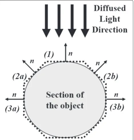
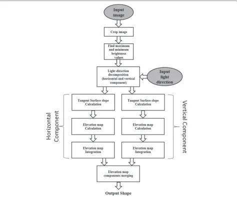
Given the two aforementioned assumptions, the amount of light reflected by one point in the observed object surface will be proportional to the angle between the normal (n) to the tangent surface in this point and the light direction. Thus, all points in whichnis parallel to the light direction (as (1) in Figure 1) are supposed to be represented in the image as the ones with maxi-mum brightness (i.e., these pixels provide the maximaxi-mum reflection). On the contrary, all points in which n is perpendicular to the light direction (as (3a) and (3b) in Figure 1) are represented with the minimum image brightness (i.e., these pixels do not provide reflection). The proposed algorithm can be summarized by the flow diagram in Figure 2.

First, the algorithm crops the input image following the object borders, in order to exclude the background pixels from the following computations. Cropping is performed by means of a single thresholding algorithm that, for each row of the image, finds the first and the last pixel in that row that are greater than a given threshold, representing the background level. Moreover,Fast-SfSsearches for the minimum and the maximum brightness values inside the cropped image.

(5)

Figure 2Flow diagram of the proposedFast-SfSalgorithm.

Then, the proposed algorithm computes the position in the 3D space of each pixel composing the cropped image. Considering the image surface as the x-yplane, and the

zaxis as the normal to the image plane, the position of a pixel in the 3D space is defined exploiting the associated

(x, y, z)coordinates. Obviously, the first two coordinates (i.e.,xandy) are simply provided by the position of the pixel in the image surface. Instead, the elevation of each pixel (i.e., z coordinate) is defined exploiting the light direction that is provided in input as the horizontal and vertical components. These components are provided as the two angles between the axiszand the horizontal (i.e., the projection on thex-zplane) and vertical projections (i.e., the projection on the y-z plane) of the vector rep-resenting the light direction. For a better comprehension, Figure 3 shows the two components of the light direction, whereαHis the component along the horizontal axis, and

αV is the one along the vertical axis.

As shown in Figure 2, the elevation of each pixel is sepa-rately computed along the horizontal and vertical compo-nent that are finally merged together to compute the shape associate to the input image. This approach ensures the reduction of complexity of the operations to be performed and potentially allows to parallelize the computations. For the sake of brevity, in the following, the algorithm details are reported for the computations related to the horizon-tal direction only. However, the same considerations are valid for the vertical components.

The elevation of each pixel is computed in two steps according to the reflection model previously described (see Figure 1).

(6)

Figure 3Light direction decomposition.(a)On image horizontal axis.(b)On image vertical axis.

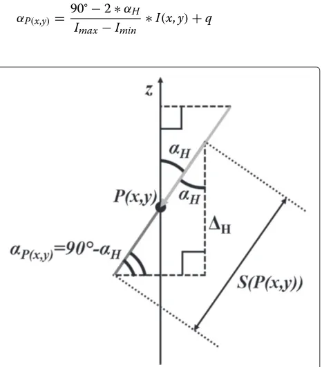
maximum brightness value in the image. In this case, the tangent surface associated toP(x,y)(S(P(x,y))) is perpen-dicular to the light direction component (i.e., like surface 1 in Figure 1), so exploiting the similar triangle theorem, it is possible to demonstrate that the slope (i,e., the angle between S(P(x,y)) and thex axis, called αP(x,y)) is equal toαH.

In the opposite case, when the considered pixel presents the minimum brightness value, the tangent surface is par-allel to the light direction (see Figure 5), andαP(x,y)is equal to 90°−αH.

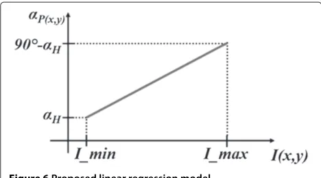
Considering that the pixels with the maximum bright-ness (Imax) have an associated angle equal to αH, and the pixels characterized by the minimum value of bright-ness (Imin) have an associated angle equal to 90° −αH,

Figure 4Case in whichP(x,y)has the maximum intensity value.

anαP(x,y)value can be assigned to all other pixels in the image by linearly regressing the range [αH; 90°−αH] on the pixel brightness range. Figure 6 shows the proposed linear regression model.

According to the graph in Figure 6, theαP(x,y)value can

be computed for each pixel as:

αP(x,y)=

90°−2∗αH

Imax−Imin ∗

I(x,y)+q

(7)

Figure 6Proposed linear regression model.

whereIx,yis the brightness value of the current pixel, and

qis equal to:

q= αH(Imax+Imin)−90°∗Imin Imax−Imin

Afterwards, in order to extract the elevation map of each pixel, i.e.,Hin Figures 4 and 5, the tangent of eachαP(x,y)

is computed. In this step, only the module of the resulting tangent value is taken into account, since from the bright-ness of a pixel it is not possible to define the sign of the slope (as surfaces (2a) and (2b) in Figure 1).

Finally, theH values are merged together to create the complete elevation map (or the object profile) associated with the horizontal component.

This is done by integrating pixel-by-pixel theH val-ues. Thus, the final elevation of each pixel is the sum of all

H associated to the pixels that precede it in the current image row. This operation is repeated for each row of the cropped image.

To discriminate if the object profile decreases or increases (i.e., ifHis positive or negative), the brightness value of the currently considered pixelI(x,y)is compared with the one of the previous in the row I(x − 1,y). If

I(x,y)≥ I, theH is considered positive (i.e., the profile of the object increases); otherwise, it is negative.

As shown in the flow diagram of Figure 2, all the aforementioned operations are repeated for the vertical component.

Finally, the two elevation map components are merged to obtain the computed shape results. The two compo-nents are combined using the following equation:

H(i,j)=

Hx(i,j)2+Hy(i,j)2

whereH(i,j)represents the output elevation map matrix,

Hx andHy are the two components of the elevation map in the horizontal and vertical axis, respectively, while

(i,j)represents the pixel position in the image.

The most complex operation that the algorithm must perform is represented by the tangent computation. How-ever, to allow a fast execution, this function can be approx-imated using a LUT approach. Moreover, compared to the SfS algorithms introduced in the previous section, Fast-SfSis not iterative, it does not present any minimization function, and it can be parallelized.

Obviously, Fast-SfS presents the same problems, in terms of output results, as all the other SfS algorithms that rely on the Lambertian surface model. Nonetheless, these problems can be overcome, resorting to stereo-vision depth measures [15,16].

Proposed hardware architecture

The overall architecture of the proposed system is shown in Figure 7. It is mainly composed of theFPGA subsystem

and theprocessor subsystem.

Thestereo-vision cameraprovides in output two 1024× 1024 grayscale images, with 8 bit-per-pixel resolution. The camera is directly connected to theFPGA subsystem(i.e., an FPGA device), that is in charge of acquiring the two images at the same time, and pre-processing them in order to enhance their quality. Moreover, the FPGA also imple-ments a feature-based matching algorithm to provide a ‘sparse’ depth map of the observed object (i.e., it pro-vides depth information of extracted features, only). In parallel to the feature-based matching algorithm, the pro-cessor subsystem performs the novel fast SfS algorithm, presented in the previous section, and provides in out-put the reconstructed shape of the actual observed object portion. The FPGA and the processor subsystems share an external memory, used to store results and temporary data, and they communicate between each other in order to avoid any collision during memory reads or writes. As aforementioned, the results obtained by the stereo-vision algorithm can be merged to the ones in output from the

Fast-SfSalgorithm to correct them and to enhance their accuracy [15,16].

(8)

The following subsections detail the functions and the internal architecture of the two subsystems.

FPGA subsystem

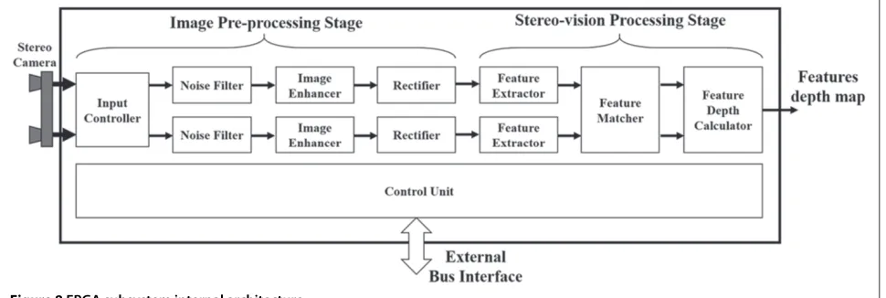
As depicted in Figure 8, theFPGA subsystemis composed of an FPGA device which includes several hardware-implemented modules.

Its internal architecture can be split in two main stages. The first, calledimage pre-processing stage, encloses the

input controller, the noise filters, the image enhancers, and the rectifiers, while the second, called stereo-vision processing stage, includes thefeature extractors, the fea-ture matcher, and the feature depth calculator. More-over, a main control unit coordinates all the activities of the different modules, providing also the interface with the external bus to communicate with the shared memory.

An FPGA-based hardware implementation of these algorithms has been preferred with respect to a soft-ware implementation running on an embedded proces-sor since, when dealing with 1024×1024 pixels images, the software alternative can lead to execution times in the order of tens of seconds (see Section ‘Experimen-tal results’ for further details). On the contrary, custom FPGA-based hardware acceleration of these algorithms can lead to very high performances.

The data stream from the stereo camera is managed by the input controller (Figure 8). The input controller

manages the communication between the stereo cam-era and the FPGA subsystem, depending on the pro-tocol supported by the camera. Moreover, it provides two output data streams, each one associated to one of the two acquired images. Each pixel stream is organized in 8-bit packets. Since the camera has a resolution of 8 bit-per-pixel (bpp), every output packet contains one pixel. The output packets associated with the right and left image are provided in input to the two noise filter

modules.

The two noise filter instances apply Gaussian noise filtering [41] on the two received images. Image noise filtering is essential to reduce the level of noise in the input images, improving the accuracy of the subsequent feature extraction and matching algorithms. In our architecture, Gaussian filtering is performed via a two-dimensional convolution of the input image with a 7×7 pixels Gaussian kernel mask [41], implementing the following equation:

FI(x,y)=

Since two-dimensional (2D) convolution is a very com-putational intensive task, to allow very fast processing, an optimized architecture has been designed. Figure 9 shows thenoise filterinternal architecture.

An assumption is that the pixels are received in a raster format, line-by-line from left to right and from top to bottom. Pixels are sent to theimage pixel organizer that stores them inside therows buffer(RB) before the actual convolution computation. RB is composed of 7 FPGA block-RAMs (BRAMs) hard macros [42], each one able to store a full image row. The number of rows of the buffer is dictated by the size of the used kernel matrix (i.e., 7×7). Rows are buffered into RB using a circular pol-icy, as reported in Figure 10. Pixels of a row are loaded from right to left, and rows are loaded from top to bottom. When the buffer is full, the following pixels are loaded, starting from the first row again (Figure 10).

The image patch selector works in parallel with the

image pixel organizer, retrieving a set of consecutive 7×7 image blocks from RB, following a sliding window

(9)

Figure 9Noise filter internal architecture.

approach on the image. Theimage patch selectoractivity starts when the first seven rows of the image are loaded in RB. At this stage, pixels of the central row (row number 4) can be processed and filtered. It is worth to remember here that, using a 7×7 kernel matrix, a 3-pixel wide border of the image is not filtered, and related pixels are there-fore discarded during filtering. At each clock cycle, a full

RB column is shifted into a 7× 7 pixelsregister matrix

(Figure 11), composed of 49 8-bit registers. After the 7th clock cycle, the first image block is ready for convolution. Thearithmetic stageconvolves it by thekernel maskand produces an output filtered pixel. At each following clock

cycle, a new RB column enters theregister matrixand a new filtered pixel of the row is produced.

While this process is carried out, new pixels continue to feed RB through theimage pixel organizer, thus imple-menting a fully pipelined computation. When a full row has been filtered, the next row can be therefore immedi-ately analyzed. However, according to the circular buffer procedure used to fill RB, the order in which rows are stored changes. Let us consider Figure 12, in which rows from 2 to 8 are stored in RB, with row 8 stored in the first position. Row 8 has to feed the last line of the

register matrix. To overcome this problem, the image patch selector includes a dynamic connection network with the register matrix. This network guarantees that, while rows are loaded in RB in different positions, the

register matrix is always fed with an ordered column of pixels.

Thearithmetic stageperforms the 7×7 matrix convo-lution using the MUL/ADD tree architecture, similar to the one presented in [43]. The tree executes 49 multipli-cations in parallel and then adds all 49 results. It contains 49 multipliers and 6 adder stages, for a total of 48 adders.

(10)

Figure 11Image patch selectorbehavior example.(a)First RB column enters in theregister matrix.(b)Pixel (4,4) is elaborated and filtered.

(11)

Finally, all filtered pixels are sent both to the image enhancerand to the externalshared memory. Storing fil-tered pixels in the external memory is mandatory since this information is needed during the following features matching phase.

Since the illumination conditions in the space environ-ment cannot be predicted a priori and, at the same time, the proposed architecture must always be able to properly work, an image enhancement is required. The enhance-ment process aims at increasing the quality of the input images in terms of illumination and contrast. In [19], it has been demonstrated that this operation allows to increase the features extraction capability, also in bad illumination conditions.

This task can be performed exploitingspatial-domain

image enhancement techniques. Among the available spatial-domain techniques, the histogram equalization

[44] is the best one to obtain a high contrasted image with an uniform tonal distribution. This technique mod-ifies the intensity value of each pixel to produce a new image containing equally distributed pixel intensity val-ues. Thus, the output images have always similar tonal distribution, reducing the effect of the illumination varia-tions. However, this technique does not work well in every condition. In fact, it works properly on images with back-grounds and foreback-grounds that are both bright or both dark (smoothed image histogram) but becomes ineffective in the other cases.

If the image histogram is peaked and narrow, the his-togram stretching [44] that allows to redistribute the pixel intensities to cover the entire tonal spectrum, provides better results. On the contrary, if the image histogram is peaked and wide, it means that the input image already has a good level of details and it contains an object on a solid color background (i.e., the image can be provided in output without modification).

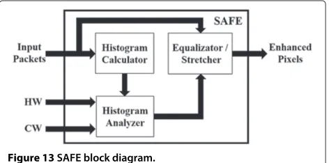
Thus, in order to design a system able to work autonomously, the image enhancer module must be able to manage these three different cases and to pro-vide in output the best enhanced image. This task can be accomplished, exploiting the hardware module pro-posed in [45], calledself-adaptive frame enhancer (SAFE), and used in [19]. SAFE is a high-performance FPGA-based IP core that is able to enhance an input image autonomously, selecting the best image enhancement technique (i.e., histogram equalization, histogram stretch-ing, or no enhancement) to be applied.

This IP core receives the input pixels from the noise filter(see Figure 8) through an 8-bit input interface (i.e., one pixel can be received each clock cycle). In addition, SAFE receives in input two parameters: HW and BW.

HW defines the threshold associated with the image his-togram width (i.e., the distance between the minimum and maximum intensity inside the image histogram).BW

defines the threshold referred to the difference between two consecutive image histogram bar (HB) values. These two parameters are required to automatically select the best image to provide in output (i.e., equalized image, stretched image, or input image without modifications), depending on the input image statistics. Figure 13 shows the block diagram ofSAFE.

The histogram calculator counts the occurrences of each pixel intensity, in order to compute the histogram bar values. In this way, when a complete image has been received, it is able to provide in output the histogram associated with the received image.

The histogram analyzer scans the image histogram in order to extract the maximum difference between two consecutive histogram bars and the histogram width. These two values are compared with the input thresholds (i.e.,HWandBW), in order to select the best image to be provided in output.

The equalizer/stretcher module performs both his-togram equalization and hishis-togram stretching on the input image, but it provides in output only the best image (i.e., equalized image, stretched image, or input image without modifications) depending on the information provided by thehistogram analyzer.

After image enhancement, the rectifier modules per-form the rectification of the left and right image, respec-tively. Image rectification is essential (i) to remove the image distortion induced by the camera lens (especially in the borders of the image) and (ii) to align the images acquired by two different points of view in order to sub-sequently apply the epipolar geometry during the feature-matching task [21]. Since the rectification parameters are fixed by the camera type and by the relative orientation between the two cameras, the rectification process can be performed using a simple LUT plus a bilinear interpola-tion approach, as done in [21,22], where the two LUTs (one for each image) are stored in the external shared memory. Basically, each input pixel in position(x,y) in the original image is moved to a new position(x1,y1)in the new rectified image. The value of the rectified pixel is computed, interpolating the four adjacent pixels in the

(12)

original image. Since for resources efficiency reasons, the LUT is stored in the external memory, and the coordinates must be translated in an absolute address value. This task is accomplished by simply adding a constant offset that is equal to the memory base address at which the LUTs are stored.

After image pre-processing, the feature-based stereo-vision algorithm can be applied in order to obtain the features depth map. The algorithm performs fea-ture extraction, feafea-ture matching, and finally, feafea-ture depth computation. Among these three activities, fea-ture extraction is the most complex one. Several feafea-ture extraction algorithms have been proposed in the litera-ture. Beaudet [46], smallest univalue segment assimilating nucleus (SUSAN) [47], Harris [48], speeded up robust features (SURF) [49], and scale-invariant feature trans-form (SIFT) [50] are just some examples. In [19], we used a software implementation of SIFT as feature extrac-tor since, from the algorithmic point of view, along with SURF, it is probably the most robust solution due to its scale and rotation invariance. This means that fea-tures can be matched between two consecutive frames even if they have differences in terms of scale and rota-tion. However, due to their complexity, their hardware implementations are very resource hungry, as reported in [51-53]. Among the available feature extraction algo-rithms, Harris is probably the best trade-off between precision and complexity [54]. In this specific case, since the two images acquired by the two cameras can present only very small differences in terms of rotations and almost no differences in terms of scale, its accuracy is comparable to the one provided by SURF and SIFT. Its complexity makes it affordable for a fast FPGA-based hardware implementation requiring limited hardware resources.

For each pixel (x,y) of a frame, the Harris algorithm computes the so-calledcorner response R(x,y)according to the following equationa:

R(x,y)=Det(N(x,y))−k·Tr2(N(x,y))

where k is an empirical correction factor equal to 0.04, andN(x,y)is the second-moment matrix, which depends on the spatial image derivativesLx andLy, in the respec-tive directions (i.e., x and y) [48]. Pixels with high corner response have high probability to represent a cor-ner (i.e., an image feature) of the selected frame and can be selected to search for matching points between consecutive frames.

Thefeatures extractorsin Figure 8 implement the Harris corner detection algorithm [48]. It is worth noting that the spatial image derivatives of the filtered image in the horizontal (Lx) and vertical (Ly) direction are per-formed by convolving the pre-processed image, read-out

from theshared memory, with the 3×3 Prewitt kernels [41], using an architecture similar to the one proposed for the noise filters, guaranteeing high throughput. The extracted features are stored inside an internal buffer, implemented resorting to the FPGA internal memory resources.

Thefeatures matcherreads from the internal buffer the features extracted by thefeatures extractorsand finds the set of features that match in the two input images, using a cross-correlation approach. Thanks to the rectification process, the features matcher must compute the cross-correlation between features belonging to the same row in the two images (1-dimensional problem), only. The formula to compute the cross-correlation between two features is:

C=

i,j∈patch

|I2(i,j)−I1(i,j)|

where patch identifies the pixels window on which the correlation must be calculated (i.e., correlation window) andI1andI2 identify the pixel intensity associated with the two input images. The less is the value ofC, the more correlated will be the two points.

The computed cross-correlation results are thresholded, in order to eliminate uncorrelated features couples. If the calculated cross-correlation value is less than a given threshold, the coordinates of the correlated features are stored inside an internal buffer.

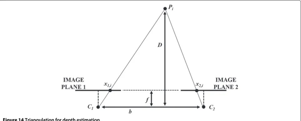
Finally, the feature depth calculator reads the coordi-nates of the matched features and computes their depth exploiting triangulation [27]. Since matched features are aligned in the two images, the triangulation becomes a 2D problem. Looking at Figure 14, knowing the focal length of the two cameras, the depthDiof a feature pointPi, i.e., the distance between the point and the baselinebof the stereo camera, can be computed as:

Di=

f ·b x1,i−x2,i

wherex1,iandx2,irepresent thex-coordinate of the con-sidered matched featurePiin the two acquired images.

Finally, the depth results are stored in the external

shared memoryin order to be accessible by theprocessor subsystemfor following computations.

Processor subsystem

(13)

Figure 14Triangulation for depth estimation.

been preferred to highlight the differences, in terms of execution time, with respect to other state-of-the-art SfS algorithms.

To perform the proposed approach, the processor reads from the shared memory one of the two rectified images. The results of the algorithm represent the shape of the observed object, with respect to a reference plane.

Eventually, the same processor subsystem can be exploited to execute the algorithm that aims at merg-ing the depth information gathered from the FPGA subsystem, with the results obtained by the fast SfS approach. This can allow (i) to correct the reconstructed shape in the features points neighbourhoods and (ii) to extract the absolute size and distance of the object under evaluation.

Experimental results

To prove the feasibility of the proposed architecture, we implemented both theFPGA subsystemand the proces-sor subsystem on a single FPGA device exploring the Aeroflex Gaisler GR-CPCI-XC4V development board, which is equipped with a XilinxVirtex-4 VLX100FPGA device and a 256 MB SDRAM memory [55]. The choice of using a Virtex-4 FPGA, instead of a more advanced device, fits the considered space debris removal applica-tions. In fact, modern radiation-hardened space-qualified FPGAs exploit the same device architecture [56]. More-over, theprocessor subsystemhas been implemented using the Aeroflex GaislerLEON3soft-core processor that rep-resents the standard processor architecture used in space applications [17].

In the following, experimental results are separately reported for the FPGA subsystem and the processor subsystem.

FPGA subsystem results

All modules described in the previous sections have been synthesized and implemented on the chosen FPGA device, resorting to XilinxISE Design Suite 14.6. Table 1 reports the resources consumption of each module com-posing theFPGA subsystem, in terms of LUTs, registers (FFs), and internal BRAMs [42].

The numbers in brackets represent the percentages of resources used with respect to the total available in the FPGA device. It is worth noting thatnoise filters, image enhancers,rectifiers, andfeatures extractorsare instanti-ated twice in the design.

To emulate the camera, the images are supposed to be pre-loaded in an external memory. Thus, theinput con-troller consists of a direct memory access interface that autonomously reads the images pre-loaded into theshared memory.

Table 1 FPGA subsystem modules logic and memory hardware resources consumption for a Xilinx Virtex-4 VLX100 FPGA device

LUTs FFs BRAM

Input controller 352 96

-Noise filter (×2) 11,792 1,392 14

Image enhancer (×2) 2,635 317 16

Rectifier (_×2) 1,216 712 8

Features extractor (×2) 19,162 2,212 12

Features matcher 2,432 656 19

Features depth calculator 615 64

-Overall 38,204 5,449 69

(14)

The entire processing chain is able to process a couple of images and to provide the associated depth map in about 32 ms, leading to a throughput of 31 image couples per second.

The bottleneck of the system is represented by the externalshared memorythat in some time slots is simulta-neously requested by different modules. Using a dual-port memory can help to avoid the stall of the processing chain, leading to a greater throughput.

To highlight the speed-up obtained by resorting to hard-ware acceleration, the algorithm implemented by the pro-posed hardware modules has also been described in C and compiled (using the maximum possible optimization level) for theLEON3processor. The processor has been implemented, enabling the floating-point unit and the internal data/instruction cache memories of 4 and 16 KB, respectively. The overall software execution time attests around 42 s, when the processor runs at 60 MHz (i.e., the maximum operating frequency of the LEON3 pro-cessor implemented on the selected FPGA device). The major contribution in the execution time is given by the Gaussian filtering and feature extraction functions that perform 2D convolution.

Comparing the overall software and hardware execu-tion times, hardware acceleraexecu-tion provides a speed-up of 1,300×.

Finally, focusing on the features extractor and fea-tures matcher modules, we can highlight the gain, in terms of hardware resources consumption, of using the

Harris algorithm, with respect to more complex SIFT

or SURF extractors. As an example, [51] and [52] pro-pose two FPGA-based implementations of the SURF algorithm. The architecture proposed in [51] consumes almost 100% of the LUTs available on a medium-sized Xilinx Virtex 6 FPGA, without guaranteeing real-time performances. Similarly, the architecture proposed in [52] consumes about 90% of the internal memory of a Xilinx Virtex 5 FPGA. It saves logic resources, but it is able to process in real-time only images with a limited resolution of 640×480 pixels. Another exam-ple is presented in [53] where an FPGA-based imexam-ple- imple-mentation of the SIFT algorithm is presented. It is able to process in real-time 640 × 480 pixel images, consuming about 30,000 LUTs and 97 internal digi-tal signal processor hard macros in a Xilinx Virtex 5 FPGA. Instead, taking into account the reduced com-plexity of the Harris algorithm, the feature extraction for the two 1024 × 1024 input images, and the match-ing task can be performed in real-time usmatch-ing only 21,594 LUTs and 31 BRAMs resources, representing the 22% and the 12.9% of the considered Virtex-4 FPGA device, respectively.

An explicit comparison with other state-of-the-art FPGA-based stereo-vision architecture has not

been made since they focus on block-based methods [28-31]. Even if they provide more dense results, due to their increased complexity, they incur in a greater hardware resources consumption (not includ-ing the resources needed for the image pre-processinclud-ing) [28,52,53].

Processor subsystem results

Theprocessor subsystemhas been implemented resorting to theLEON3soft-core processor architecture [17] and integrated in the same FPGA device as theFPGA subsys-tem. The processor has been implemented, enabling the floating-point unit and the internal data and instruction cache memories of 4 and 16 KB, respectively. The max-imum operating frequency of the processor, synthesized on a Xilinx Virtex-4 VLX 100 FPGA device, is equal to 60 MHz.

The chosen processor configuration leads to an hard-ware resources usage of 21,395 LUTs, 8,750 FFs, and 32 BRAMs. Thus, the overall resources consumption of the proposed system (FPGA and processor subsystems) is around 60% of the overall logic resources available in the FPGA device.

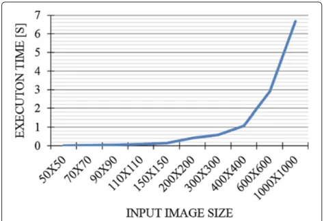
In order to evaluate the execution time of the pro-posedFast-SfSalgorithm, different executions have been performed on the LEON3processor, providing in input images with different size. The graph in Figure 15 shows the execution time trend with respect to the input image size.

The proposed algorithm has been compared, in terms of execution time, to other SfS approaches proposed in the literature. Durou et al. [33] reports execution times of the fastest SfS algorithms presented in the literature. The algorithms are executed on a Sun Enterprise E420

(15)

machine [57], equipped with four UltraSparc II processors running at 450 MHz, each one with 4 MB of dedicated cache. From [33], the fastest SfS algorithm is the one pre-sented in [58], that is an iterative algorithm, requiring 0.29 s for 5 iterations and 1.17 for 20 iterations (to ensure better results), to process a 256 × 256 images. Even if running on a processor running at 1/6 of the operat-ing frequency and equipped with a cache of 3 orders of magnitude smaller, the algorithm proposed in this paper requires almost the same time of [58].

In [34], authors state that the proposed non-iterative SfS algorithm is faster than the iterative ones. By compar-ing their approach withFast-SfS, from Figure 16, it can be seen that the speed-up is always greater than 3×. It is worth noting that in [34], the testbed used to run the proposed algorithm is not defined.

Finally, Figures 17, 18 and 19 depict the results obtained by running the proposedFast-SfSalgorithm on a 200×200 synthetic image representing a semi-sphere, on a 400× 600 synthetic image representing a vase, and on a 459× 306 real image representing a drinking bottle. This last test image has been chosen since its shape is more similar to a space debris.

The algorithm applied on the two synthetic images provides good results since they are characterized by a diffused light and a monochromatic surface. This char-acteristics completely match the assumptions on which the proposed algorithm is based (see Section ‘Novel fast shape-from-shading algorithm’).

On the other hand, in the real image the target object is illuminated by direct light, since diffused light can-not be easily reproduced in laboratory. Moreover, due to the reflective material composing the object, the image presents some light spots (see the upper central part of the drinking bottle in Figure 19a). As can be noted in Figure 19b,c, these light spots lead to some peaks in the

Figure 16Comparison of the execution times ofFast-SfSand the algorithm reported in [34].

Figure 17ExampleFast-SfS output result on the semi-sphere image.(a)Input image.(b)Fast-SfSresults (side view).(c)Fast-SfS results (dimetric view).

(16)

Figure 18ExampleFast-SfS output result on the vase image.(a)Input image.(b)Fast-SfSresults (dimetric view).(c)Fast-SfSresults (opposite dimetric view).

Conclusions

This paper presented a novel fast SfS algorithm and an FPGA-based system architecture for video-based shape reconstruction to be employed during space debris removal missions. The FPGA-based architecture provides fast image pre-processing, depth information exploiting

a feature-based stereo-vision approach, and SfS results employing a processor that executes the proposed novel SfS algorithm.

(17)

Figure 19ExampleFast-SfS output result on the drinking bottle image.(a)Input image.(b)Fast-SfSresults (front view, highlighting the light spots).(c)Fast-SfSresults (oblique view).

hardware resources consumption of the entire system allows to implement it in a single FPGA device, leaving free more than the 40% of overall hardware resources in the selected device.

The remaining part of the FPGA device can be exploited (i) to improve the reliability of the design, employed in space applications, e.g., applying some fault tolerance techniques; (ii) to hardware accelerate the proposed SfS algorithm, avoiding the usage of a processor; and (ii) to include the following vision-based algorithms that aim at merging the results obtained by the stereo-vision and the novel fast SfS approach.

When more detailed requirements of the space debris removal missions will be available, future work will focus on the improvement of the proposed algorithm, taking also into account the earth albedo effect during the shape model computation.

Endnote

a_Det₍_X₎_{denotes the determinant of matrix}_X_{, and}

Tr(X)denotes the trace of matrixX

Competing interests

(18)

Acknowledgements

The authors would like to express their sincere thanks to Dr. Walter Allasia and Dr. Francesco Rosso of Eurix company for their helpful hints and fruitful brainstorming meetings.

Received: 28 February 2014 Accepted: 12 September 2014 Published: 25 September 2014

References

1. European Space Agency (ESA): Requirements on Space Debris Mitigation for ESA Projects (2009). http://iadc-online.org/References/Docu/ESA %20Requirements%20for%20Space%20Debris%20Mitigation.pdf 2. NASA Headquarters Office of Safety and Mission Assurance, NASA

Technical Standard: Process for Limiting Orbital Debris.National Aeronautics and Space AdministrationNASA-STD8719.14, Washington DC (USA), (2011) http://www.hq.nasa.gov/office/codeq/doctree/871914.pdf 3. Steering Group, Key Definitions of the Inter-Agency Space Debris

Coordination Committee (IADC). Inter-Agency Space Debris Coordination Committee (IADC)IADC-13-02 (2013) http://www.iadc-online.org/ Documents/IADC-2013-02,%20IADC%20Key%20Definitions.pdf 4. R Piemonte, CApture and DE-orbiting Technologies (CADET) project.

http://web.aviospace.com/cadet/index.php/obj

5. D Kessler, Collisional cascading: The limits of population growth in low earth orbit. Adv. Space Res.11(12), 63–66 (1991)

6. C Bonnal, W Naumann, Ariane debris mitigation measures: Past and future. Acta Astronautica40(2–8), 275–282 (1997)

7. European Space Agency (ESA): Launchers. http://www.esa.int/ Our_Activities/Launchers/Ariane_42

8. MH Kaplan, Space debris realities and removal, inProceedings of Improving Space Operations Workshop (SOSTC) 2010(Greenbelt (MD, USA), 2010) 9. N Zinner, A Williamson, K Brenner, JB Curran, A Isaak, M Knoch, A Leppek,

J Lestishen, Junk hunter: Autonomous rendezvous, capture, and de-orbit of orbital debris, inProceedings of AIAA SPACE 2011 Conference & Exposition (Pasadena (CA, USA), 2011)

10. F ter Haar,Reconstruction and analysis of shapes from 3d scans, PhD thesis. (Utrecht University, 2009)

11. A Kato, LM Moskal, P Schiess, ME Swanson, D Calhoun, W Stuetzle, Capturing tree crown formation through implicit surface reconstruction using airborne lidar data. Remote Sensing Environ.113(6), 1148–1162 (2009)

12. Y Tang, X Hua, M Yokomichi, T Kitazoe, M Kono, Stereo disparity perception for monochromatic surface by self-organization neural network, inNeural Information Processing, 2002. ICONIP ’02. Proceedings of the 9th International Conference On, vol. 4 (Singapore (Malaysia), 2002), pp. 1623–16284

13. R Zhang, P-S Tsai, JE Cryer, M Shah, Shape-from-shading: a survey. Pattern Anal. Mach. Intell. IEEE Trans.21(8), 690–706 (1999)

14. S Kumar, M Kumar, B Raman, N Sukavanam, R Bhargava, Depth recovery of complex surfaces from texture-less pair of stereo images. Electron. Lett. Comput. Vis. Image Anal.8(1), 44–56 (2009)

15. MV Rohith, S Sorensen, S Rhein, C Kambhamettu, Shape from stereo and shading by gradient constrained interpolation, inImage Processing (ICIP), 2013 20th IEEE International Conference On(Melbourne, 2013),

pp. 2232–2236

16. CK Chow, SY Yuen, Recovering shape by shading and stereo under lambertian shading model. Int. J. Comput. Vis.85(1), 58–100 (2009) 17. J Gaisler, A portable and fault-tolerant microprocessor based on the sparc

v8 architecture, inDependable Systems and Networks, 2002. DSN 2002. Proceedings. International Conference On(IEEE Bethesda (MD, USA), 2002), pp. 409–415

18. S Habinc,Suitability of reprogrammable FPGAs in space applications -feasibility report, Technical report. (Gaisler Research, Gothenburg (Sweden), 2002)

19. F Rosso, F Gallo, W Allasia, E Licata, P Prinetto, D Rolfo, P Trotta, A Favetto, M Paleari, P Ariano, Stereo vision system for capture and removal of space debris, inDesign and Architectures for Signal and Image Processing (DASIP), 2013 Conference On(IEEE, Cagliari (Italy), 2013), pp. 201–207

20. R Hartley, A Zisserman,Multiple View Geometry in Computer Vision. (Cambridge university press, Cambridge, 2003)

21. C Vancea, S Nedevschi, Lut-based image rectification module implemented in fpga, inIntelligent Computer Communication and

Processing, 2007 IEEE International Conference On(IEEE, Cluj-Napoca (Romania), 2007), pp. 147–154

22. DH Park, HS Ko, JG Kim, JD Cho, Real time rectification using differentially encoded lookup table, inProceedings of the 5th International Conference on Ubiquitous Information Management and Communication(ACM, Seoul (Republic of Korea), 2011), p. 47

23. H Sadeghi, P Moallem, SA Monadjemi, Feature based color stereo matching algorithm using restricted search, inProceedings of the European Computing Conference(Springer, Netherland, 2009), pp. 105–111 24. CJ Taylor, Surface reconstruction from feature based stereo, inComputer

Vision, 2003. Proceedings. Ninth IEEE International Conference On(IEEE Kyoto (Japan), 2003), pp. 184–190

25. Y-S Chen, Y-P Hung, C-S Fuh, Fast block matching algorithm based on the winner-update strategy. Image Process. IEEE Trans.10(8), 1212–1222 (2001)

26. I Nahhas, M Drahansky, Analysis of block matching algorithms with fast computational and winner-update strategies. Int. J. Signal Process. Image Process. Pattern Recognit.6(3), 129 (2013)

27. N Ayache,Artificial Vision for Mobile Robots: Stereo Vision and Multisensory Perception. (MIT Press, Cambridge, 1991)

28. C Colodro-Conde, FJ Toledo-Moreo, R Toledo-Moreo, JJ Martínez-Álvarez, J Garrigós Guerrero, JM Ferrández-Vicente, Evaluation of stereo correspondence algorithms and their implementation on fpga. J. Syst. Arch.60(1), 22–31 (2014)

29. S Thomas, K Papadimitriou, A Dollas, Architecture and implementation of real-time 3d stereo vision on a xilinx fpga, inVery Large Scale Integration (VLSI-SoC), 2013 IFIP/IEEE 21st International Conference On(IEEE, Istanbul (Turkey), 2013), pp. 186–191

30. W Wang, J Yan, N Xu, Y Wang, F-H Hsu, Real-time high-quality stereo vision system in fpga, inField-Programmable Technology (FPT), 2013 International Conference On(IEEE, Kyoto (Japan), 2013), pp. 358–361 31. P Zicari, H Lam, A George, Reconfigurable computing architecture for

accurate disparity map calculation in real-time stereo vision, inIn Proc. International Conference on Image Processing, Computer Vision, and Pattern Recognition (IPCV’13), vol. 1, (2013), pp. 3–10

32. BKP Horn, MJ Brooks (eds.),Shape from Shading. (MIT Press, Cambridge, 1989)

33. J-D Durou, M Falcone, M Sagona, A survey of numerical methods for shape from shading. Institut de Recherche en Informatique (IRIT) Université Paul Sabatier, Rapport de rechercheIRITN2004-2-R (2004) 34. R Szeliski, ed. by OD Faugeras, Fast shape from shading, inECCV. Lecture

Notes in Computer Science, vol. 427 (Springer US, 1990), pp. 359–368 35. P Daniel, J-D Durou, From deterministic to stochastic methods for shape

from shading, inIn Proc. 4th Asian Conf. on Comp. Vis(Taipei (China), 2000), pp. 187–192

36. L Abada, S Aouat, Solving the perspective shape from shading problem using a new integration method, inScience and Information Conference (SAI), 2013(London (UK), 2013), pp. 416–422

37. NASA Earth Observatory: Global Albedo. http://visibleearth.nasa.gov/ view.php?id=60636

38. The U.S. Geological Survey USGS Water Science School: How much water is there on, in, and above the Earth? http://water.usgs.gov/edu/ earthhowmuch.html

39. N Xie, AJP Theuwissen, An autonomous microdigital sun sensor by a cmos imager in space application. Electron Devices IEEE Trans.59(12), 3405–3410 (2012)

40. CR McBryde, EG Lightsey, A star tracker design for cubesats, inAerospace Conference, 2012 IEEE(Big Sky (MT - USA), 2012), pp. 1–14

41. RC González, RE Woods,Digital Image Processing. (Pearson/Prentice Hall, US, 2008)

42. Xilinx Corporation: Virtex-4 FPGA User Guide - UCG070. (2008). http://www.xilinx.com/support/documentation/user_guides/ug070.pdf 43. S Di Carlo, G Gambardella, M Indaco, D Rolfo, G Tiotto, P Prinetto, An

area-efficient 2-D convolution implementation on FPGA for space applications, inProc. of 6th International Design and Test Workshop (IDT) (Beirut (Lebanon), 2011), pp. 88–92

(19)

45. S Di Carlo, G Gambardella, P Lanza, P Prinetto, D Rolfo, P Trotta, Safe: a self adaptive frame enhancer fpga-based ip-core for real-time space applications, inProc. of 7th International Design and Test Workshop (IDT) (Doha (Qatar), 2012)

46. P Beaudet, Rotationally invariant image operators, inProc. of 4th International Joint Conference on Pattern Recognition(Kyoto (Japan), 1978), pp. 579–583

47. SM Smith, JM Brady, SUSAN - a new approach to low level image processing. Int. J. Comput. Vis. (IJCV)23, 45–78 (1995)

48. C Harris, M Stephens, A combined corner and edge detector, inProc. of the 4th Alvey Vision Conference(Manchester (United Kingdom), 1988), pp. 147–151

49. H Bay, A Ess, T Tuytelaars, LV Gool, SURF: Speeded up robust features. Comput. Vis. Image Underst. (CVIU)110, 346–359 (2008)

50. DG Lowe, Object recognition from local scale-invariant features, in Proceedings of the International Conference on Computer VisionVolume 2 -Volume 2. ICCV ’99(IEEE Computer Society, Washington, 1999) 51. N Battezzati, S Colazzo, M Maffione, L Senepa, SURF algorithm in FPGA: a

novel architecture for high demanding industrial applications, inProc. of 2012 Design, Automation Test in Europe Conference Exhibition (DATE) (Dresden (Germany), 2012), pp. 161–162

52. D Bouris, A Nikitakis, I Papaefstathiou, Fast and efficient fpga-based feature detection employing the surf algorithm, inField-Programmable Custom Computing Machines (FCCM) 2010 18th IEEE Annual International Symposium On(Toronto (Canada), 2010), pp. 3–10

53. L Yao, H Feng, Y Zhu, Z Jiang, D Zhao, W Feng, An architecture of optimised SIFT feature detection for an fpga implementation of an image matcher, inField-Programmable Technology, 2009. FPT 2009. International Conference On(Sydney (Australia), 2009), pp. 30–37

54. T Tuytelaars, K Mikolajczyk, Local invariant feature detectors: a survey. Foundations Trends Comput. Graph. Vis.3(3), 177–280 (2008)

55. Gaisler Research AB: GR-CPCI-XC4V LEON PCI Virtex 4 Development Board - Product sheet. (2007).

http://www.pender.ch/docs/GR-CPCI-XC4V_product_sheet.pdf

56. Xilinx Corporation: Space-Grade Virtex-4QV Family Overview - DS653. (2010). http://www.xilinx.com/support/documentation/data_sheets/ ds653.pdf

57. Inc SM, Sun Enterprise 420R Server Owner’s Guide. (1999). http://docs. oracle.com/cd/E19088-01/420r.srvr/806-1078-10/806-1078-10.pdf 58. Ping-T Sing, M Shah, Shape from shading using linear approximation.

Image Vis. Comput.12(8), 487–498 (1994)

doi:10.1186/1687-6180-2014-147

Cite this article as:Di Carloet al.:A novel algorithm and hardware

architecture for fast video-based shape reconstruction of space debris. EURASIP Journal on Advances in Signal Processing20142014:147.