Technological Progress and Economic Transformation

(1)

NBER WORKING PAPER SERIES

TECHNOLOGICAL PROGRESS AND ECONOMIC TRANSFORMATION Jeremy Greenwood

Ananth Seshadri Working Paper 10765

http://www.nber.org/papers/w10765

NATIONAL BUREAU OF ECONOMIC RESEARCH 1050 Massachusetts Avenue

Cambridge, MA 02138 September 2004

This survey paper has been prepared for the Handbook of Economic Growth edited by Philippe Aghion and Steven Durlauf (North-Holland, Amsterdam). Matthias Doepke, Nezih Guner and Baris Kaymak are thanked for comments. Financial support from the NSF (award number 0136055) is gratefully acknowledged. The views expressed herein are those of the author(s) and not necessarily those of the National Bureau of Economic Research.

©2004 by Jeremy Greenwood and Ananth Seshadri. All rights reserved. Short sections of text, not to exceed two paragraphs, may be quoted without explicit permission provided that full credit, including © notice, is given to the source.

(2)

Technological Progress and Economic Transformation Jeremy Greenwood and Ananth Seshadri

NBER Working Paper No. 10765 September 2004

JEL No. D1, E1, J1, O3

ABSTRACT

Growth theory can go a long way toward accounting for phenomena linked with U.S. economic development. Some examples are:

(i) the secular decline in fertility between 1800 and 1980,

(ii) the decline in agricultural employment and the rise in skill since 1800, (iii) the demise of child labor starting around 1900,

(iv) the increase in female labor-force participation from 1900 to 1980, (v) the baby boom from 1936 to 1972.

Growth theory models are presented to address all of these facts. The analysis emphasizes the role of technological progress as a catalyst for economic transformation.

Jeremy Greenwood Department of Economics University of Rochester P.O. Box 270156 Rochester, NY 14627-0156 and NBER gree@troi.cc.rochester.edu Ananth Seshadri Department of Econonmics University of Wisconsin Madison, WI 53706-1393 aseshadri@ssc.wisc.edu

(3)

1 Introduction

Life in the 1800’s: Imagine living as a typical American child in the nineteenth century. You have six brothers and/or sisters. You live in a house, outside of an urban area, with no running water, no central heating, and no electricity. Your father labors 70 hours a week in the agricultural economy. Your mother probably puts in about the same amount of time doing work at home. Less than half of your years between the ages of 5 and 20 will be devoted to school. So, perhaps you are playing in the family kitchen that contains a cast iron range, a table, and a dresser. But, more likely you are helping your parents by doing one of a litany of chores: carrying wood or water into the house, washing clothes on a scrub board or ironing them with a flat iron, looking after younger siblings, preparing meals, cleaning the house, making clothes, tending crops or animals, etc. In this era, household production is an incredibly labor-intensive process. What changed this situation? The catalyst for the ensuing economic transformation to modern day life was technological progress, both in the market and at home, or so it will be argued here.

1.1 Technological Progress in the Market

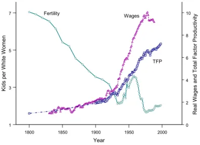
Fertility: Over the period from 1830 to 1990 real wages increased by a factor of 9 — see Figure 1.1 This rise was propelled by a near 7-fold increase in market-sector total factor productivity (TFP) between 1800 and 1990. Such tremendous technological advance had a dramatic impact on everyday life. As an example, consider the eﬀect that economic progress could have had on fertility. Raising children takes time. A secular increase in real wages implies that the opportunity cost of having a child, when measured in terms of market goods, will rise. The utility value of an extra unit of market consumption relative to an extra child should fall, however, as market goods become more abundant with economic development. So long as the marginal utility of market goods falls by less than the increase in real wages fertility should decline. And so fertility did decline, from 7 kids per woman in 1800 to 2

(6)

1800 1850 1900 1950 2000 Year 1 3 5 7 K ids pe r W hi te W om e n 0 2 4 6 8 10 R eal Wag e s and Total Factor Prod uctivity Fertility _Wages TFP

Figure 1: Technological Progress in the Market and Fertility today.

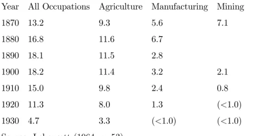
Industrialization and Skilled Labor: At the start of the 1800’s America was largely a rural economy. Over seventy percent of workers were employed in agriculture — see Figure 2.2

Less than 50 percent of children between the ages of 5 and 20 went to school. From 1800 to1940 technological advance in the nonagricultural sector of the U.S. economy was twice as fast as in the agricultural sector. Furthermore, agricultural goods had a lower income elasticity than nonagricultural ones. These two facts together implied that the demand for labor in the nonagricultural sector of the economy rose relative to the demand for labor in the agricultural sector. Since the nonagricultural sector required a more skill-intensive labor force than did the agricultural sector, the demand for skilled labor rose too.

Child Labor: Children formed an important part of the labor force in the nineteenth century. Exact numbers are hard to come by, though. First, the data before 1870 is scarce. Lebergott (1964, p. 50) reports that 43 percent of textile workers in Massachusetts around 2 _{The enrollment rate} _{figures come from} _{Historical Statistics of the United States: Colonial Times to}

1970 (1975, Series H 433). See Greenwood and Seshadri (2002) for the sources of the other data plotted in Figure 2.

(7)

1800 1850 1900 1950 0 20 40 60 80 Sh are of Emplo yment in Agri culture , % 50 60 70 80 90 Enrol lm ent Rate, % Empl. 1800 1850 1900 1950 1 2 3 4 5 6 7 TFP -- agri. TFP -- manu. School

Figure 2: The Decline in Agriculture and the Rise in Skilled Labor

1820 were children, as were 47 and 55 percent in Connecticut and Rhode Island. Second, the availablefigures pertain to paid labor. These statistics omit the labors of children on family farms and businesses, or around the home — the same is true for the housewives of the era. The incidence of child labor rose until 1900, as Table 1 shows. At that time children made up about 20 percent of the paid labor force. It then began to decline. By 1930 child labor had vanished.

A reasonable hypothesis is that technological progress reduced the need for unskilled labor in agriculture and manufacturing. Take agriculture, for example, where the late nineteenth and early twentieth centuries saw massive improvements in agricultural technology. Two of the most important inventions were the horse-drawn harvester in the mid-nineteenth century and the tractor that began to diﬀuse into American farms in the early twentieth century. Mechanization of farms virtually eliminated the need for raw labor: In 1830, it would take a farmer 250-300 hours to grow 100 bushels of wheat; in 1890, 40-50 hours with the help of a horse-drawn machine; in 1930, 15-20 hours with a tractor; and in 1975, 3-4 hours with large tractors and combines.3

(8)

Table 1: Children aged 10-15 as Percentage of the Gainfully Employed

Year All Occupations Agriculture Manufacturing Mining

1870 13.2 9.3 5.6 7.1 1880 16.8 11.6 6.7 1890 18.1 11.5 2.8 1900 18.2 11.4 3.2 2.1 1910 15.0 9.8 2.4 0.8 1920 11.3 8.0 1.3 (<1.0) 1930 4.7 3.3 (<1.0) (<1.0) Source: Lebergott (1964, p. 53)

1.2 Technological Progress in the Home

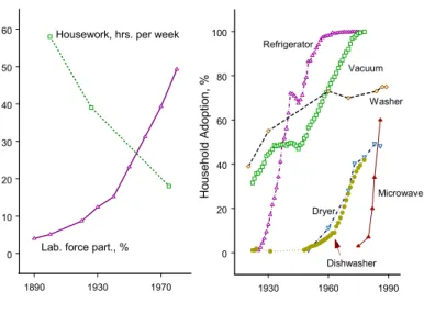
Female Labor-Force Participation: Just as the last 200 years have witnessed technological progress in the market sector, they have witnessed tremendous technological advance in the home sector. Since productivity numbers are not computed for the home sector, given the elusive nature of output and inputs, the evidence on technological progress is circumstantial. The household sector in the American economy was basically a cottage industry until the dawning of the Second Industrial Revolution. With the onset of the electric age a host of new appliances were ushered in: washing machines, refrigerators, etc. It took time for these new capital goods to diﬀuse through the economy, as Figure 3 shows.4 _{At the same time,}

the principles of scientific management were being applied to everyday household tasks. The large table and isolated dresser that characterized a kitchen of the 1800’s were replaced by continuous countertops and built-in cabinets. This wave of technological progress in the home freed up tremendous amounts of labor — see Figure 3. The time spent on housework fell from 58 hours per week in 1900 to just 18 in 1975. Married women could now enter the labor force, and they did in droves.

3 _{Source: U.S. Department of Agriculture, http://www.usda.gov/history2/text4.htm.}

(9)

1890 1930 1970 0 10 20 30 40 50 60 1930 1960 1990 0 20 40 60 80 100 Ho useh old Ad optio n, % Refrigerator Vacuum Washer Microwave Dishwasher Dryer

Housework, hrs. per week

Lab. force part., %

Figure 3: Technological Progress in the Home and Female Labor-Force Participation Fertility: Technological progress in the household sector could also have had implications for fertility. Labor-saving household goods that ease the burden of housework will lower the cost of raising children. Fertility should rise. In fact it did, between 1936 and 1957 fertility increased by 53 percent — see Figure 1.

1.3 The Goal

The goal here is to persuade you that standard Solow (1956) -cum- Ramsey (1928) growth theory can be fruitfully employed to explain these phenomena. Specifically, all of these facts can be accounted for by modifying the standard growth paradigm to incorporate fertility decisions, household production, human capital investment in children, labor-force partic-ipation, and multiple sectors. It will be argued that technological progress is the engine driving economic transformation. A selective review of the literature is provided in Section 7.

(10)

2 The Baby Bust and Baby Boom

Two facts stand out about the fertility of American women. First, it has dropped drastically over the last two hundred years. This decline is called the demographic transition, but will be labeled here the baby bust. Second, the secular decline in fertility has had only one interruption, the baby boom. These two facts can easily be accounted for within the context of the neoclassical growth model. Just two modifications to the standard model are required: a fertility decision needs to be added, and household production incorporated.

2.1 The Environment

Imagine a small open economy populated by overlapping generations.5 _{People live for three}

periods, one period as children and two as adults. Young adults are endowed with one unit of time. They can use this time for either working or raising kids. An adult is fecund only in the first period of his life. Old agents are retired.

Tastes: The lifetime utility function for a young adult is given by

φln(cy+c) +βφln(co0) + (1 +β)(1₋φ) lnny, (1)

where cy _and _co0 _{denote the adult’s consumption when young and old, and} _ny _represents the number of kids that he would like to have when young. The constant c proxies for the household production of market goods. As will be seen, it plays an important role in the analysis.

Income: Young agents work for the market wage w. They save for old age at the internationally determined time-invariantgross interest rate r.

Cost of Children: Children are expensive. The production function for children is given by

ny =x(ly)1−γ, (2)

wherely_{is the time a young adult devotes to raising children and}_x_{is the level of productivity} 5 _{The model presented here is based on Greenwood, Seshadri and Vandenbroucke (2002).}

(11)

in the home sector. The consumption cost, k, of raisingny kids is therefore given by k =w(n y x ) 1/(1−γ) .

The cost of raising children is directly proportional to the wage rate.

The Young Agent’s Choice Problem: The decision problem facing a young adult is

max cy_,co0,ny{φln(c y ₊_c_{) +}_βφ_ln(_co0_{) + (1 +}_β₎₍₁₋_φ_{) ln}_ny }, subject to cy+ c o0 r =w−w( ny x ) 1/(1−γ)_.

The Euler equation for consumption is

1

cy₊_c =βr

1

co0,

which can be rewritten as

co0 =βr(cy +c). (3)

This equation simply states that consumption of market goods over the household’s lifetime will grow at the (gross) rate βr. If the gross rate of interest, r, exceeds the gross rate of time preference, 1/β, consumption increases over the household’s lifetime, and likewise will decline whenr <1/β.

The above optimization problem can be reformulated using (3) to appear as

max cy_,ny{(1 +β)[φln(c y ₊_c_{) + (1} −φ) lnny] +βφln(βr)_}, (4) subject to cy +c= 1 1 +β[w−w( ny x ) 1/(1−γ)₊_c_]_. ₍₅₎

The first-order condition to this problem is

φ cy₊_c 1 1 +β 1 1₋γwx −1/(1−γ)₍_ny₎γ/(1−γ) ₌ (1−φ) ny . (6)

The righthand side of this equation gives the marginal benefit from having an extra kid. The lefthand side represents the marginal cost. This is the product of two components. Having

(12)

an extra child necessitates working less in the market. This will lead to a sacrifice in terms of market consumption in the amount[(1 +β)(1₋γ)]−1_wx−1/(1−γ)₍_ny₎γ/(1−γ)_{. The marginal}

utility derived from an extra unit of consumption isφ/(cy₊_c₎_.

The Firm’s Problem: Let market output, o, be produced in line with the following production function:

o=zkαl1−α,

where k and l are the inputs of capital and labor used in production and z is the level of productivity in the market sector. Now, suppose that capital depreciates fully after use in production. The rental rate on capital will then ber, since it must yield the same return as a bond. The problem facing the firm is therefore given by

max

k,l {zk α_l1−α

−rk₋wl_}.

The first-order conditions connected to this problem are

αzkα−1l1−α =r, (7)

and

(1₋α)zkαl−α=w. (8)

These first-order conditions simply state that each factor gets paid its marginal product. By substituting equation (7) into (8), it is easy to see that

w= (1₋α)αα/(1−α)z1/(1−α)r−α/(1−α). (9)

Hence, the wage rate, w, is determined by the level of market productivity, z, and the international rate of return on capital,r.

Population Growth: Let sy andso stand for the current sizes of the young and old adult populations, respectively. Since today’s young generation will be tomorrow’s old generation it must transpire that

(13)

where a prime aﬃxed to a variable denotes its value next period. Now, each young adult hasny _{kids so the size of next period’s young generation is given by}

sy0 =nysy. (11)

2.2 Analysis

Lemma 1 Fertility, ny_{, decreases with market wages,} _w_{, and increases with technological} advance in the home sector, x.

Proof. Take thefirst-order condition for ny_{, or (6), and rewrite it as}

ny =A1−γx[(c y ₊_c₎ w ] (1−γ)_, ₍₁₂₎ where A_≡ (1 +β)(1−γ)(1−φ) φ .

Plugging the above equation into the budget constraint (5) yields

cy +c= 1

1 +β+A(w+c).

Last, using the solution for cy +c in (12) generates

ny = [ A

1 +β+A]

1−γ_x_{(1 +}_c_/w₎1−γ_. ₍₁₃₎

The proof is now complete since it’s trivial to see that ny _{is decreasing in}_w_{, and increasing} in x.

Intuition: With the aid of some diagrams, it’s easy to ferret out the intuition underlying the above lemma. First, observe that (5) specifies the consumption possibilities frontier facing the household. The slope of the frontier is

d(cy₊_c₎ dny =−w( 1 x) 1/(1−γ)₍_ny₎γ/(1−γ)_/_{[(1 +}_β₎₍₁ −γ)]_≤0. (14) This is shown in Figure 4 by the concave consumption possibilities frontier, labeled P P. The frontier hits the vertical axis at the point cy ₊_c_{= [}_w₊_c_]_/_{(1 +}_β₎_{, and the horizontal} one at ny ₌_x_{(1 +}_c_/w₎(1−γ)_.

(14)

P P * y n β 1 w + +c c + * y c γ) (1 ) w x(1₊ c − c + y c y n

Figure 4: The Determination of Fertility

The objective function (4) defines indiﬀerence curves over the various (ny_{, c}y₊_c₎ combi-nations. The slope of an indiﬀerence curve is given by

d(cy₊_c₎ dny |utility constant=− (1₋φ) φ cy₊_c ny ≤0. (15)

The equilibrium level of fertility and market consumption are shown in standard fashion by the point(ny∗_{, c}y∗₊_c₎_{where the indi}_ﬀ_{erence curve is tangent to the consumption possibilities}

frontier — see Figure 4.

Let wages increase by a factor ofλand assume thatc= 0. In response, the consumption possibilities frontier will rotate upwards from the curveP P, by a factor ofλ, to the position shown by the curve P0_P _{— see Figure 5. Thus, there is a positive income e}_ﬀ_{ect associated}

with an increase in wages. The slope of the consumption possibilities curve will increase by a factor of λ at any ny _{point, too, as is evident from (14). That is, the marginal cost of} an extra child rises. This eﬀect should operate to reduce fertility. It’s easy to deduce that consumption, cy_{, will move up by a factor of} _λ _{and that fertility,} _ny_{, will remain constant.} This transpires because the substitution and income eﬀects on fertility from an increase in wages exactly cancel out, an artifice of the logarithmic form of preferences adopted in (1).

(15)

P P * y n β 1 w + * y c x _ny β 1 λw + ) λc , (ny* y* P'

Figure 5: The Eﬀect of an Increase in Wages on Fertility whenc= 0

To see this, note that along any vertical line the slopes of the indiﬀerence curves increase in proportion with the increases incy_{, as is clear from (15). The slope of the indi}_ﬀ_{erence curve} at the point(ny∗_{, λc}y∗₎_{is higher by a factor of exactly}_λ _{relative to the slope of the curve at}

the point (ny∗_{, c}y∗₎_.

Now suppose that wages jump up by a factor ofλand assume thatc>0. The consump-tion possibilities frontier no longer shifts upwards in a proporconsump-tional manner. The horizontal intercept now shifts in — see Figure 6. A higher wage rate implies that the household pro-duction of market goods, c, now frees up less time for kids. As can be seen, fertility must unambiguously fall from ny∗ _to _ny∗0_{. Why? Suppose that fertility remains} _fi_{xed at its old}

level,ny∗_{, and that consumption once again rises by a factor of}_λ_{, say from}_cy∗ _to_λcy∗_{. (Note}

thatcy∗ _and_λcy∗_{are not labeled on the diagram.) The slope of the consumption possibilities}

frontier will once again increase by a factor of λ, in line with (14). The slope of the indiﬀ er-ence curve through the point(ny∗_{, λc}y∗₊_c₎_{will increase by less, though, due to the presence}

of thec term in preferences — see (15) and the dashed indiﬀerence curve in Figure 6. Hence, a point of tangency cannot occur. At the margin a parent is willing to give up a child for

(16)

P * y n β + + 1 w c γ) (1 ) w x(1₊ c − _ny P' y*' n c + y c P P'

Figure 6: The Eﬀect of Wages on Fertility when c₆= 0

[(1₋φ)/φ](λcy∗₊_c₎_/ny∗_{units of consumption. According to his production possibilities he}

can get λw(1/x)1/(1−γ)₍_ny∗₎γ/(1−γ)_/_{[(1 +}_β₎₍₁

−γ)] units of consumption for an incremental cut in fertility. Now,[(1₋φ)/φ](λcy∗₊_c₎_/ny∗ _{< λw}₍₁_/x₎1/(1−γ)₍_ny∗₎γ/(1−γ)_/_{[(1 +}_β₎₍₁

−γ)], since [(1₋φ)/φ](cy∗ ₊_c₎_/ny∗ ₌ _w₍₁_/x₎1/(1−γ)₍_ny∗₎γ/(1−γ)_/_{[(1 +}_β₎₍₁

−γ)]. Therefore, he should cut his level of fertility. In other words, when c >0 the substitution eﬀect from an increase in w outweighs the income eﬀect.

Last, consider the effect of technological progress in the household sector. An increase in x shifts the consumption possibilities frontier outwards in the manner shown by Figure 7 (from P P to P P0_{). At any} _ny _{point the consumption possibilities curve becomes less} steep since the consumption cost of an extra kid falls. As a result, both the income and substitution effects operate to increase fertility. (Since kids are a normal good, as one moves upwards along any vertical line the slopes of the indifference curves increase. This implies that the new consumption point must lie to right ofny_.)

Corollary Fertility, ny_{, is decreasing in the level of market productivity,} _z_{. (Fertility is} increasing in the international rate of return, r.)

(17)

P P * y n β 1 w + +c γ) (1 ) w (1 x' ₊c −

n

y P' y*' n

Figure 7: The Eﬀect of an Improvement in Household Technology on Fertility Proof. Substitute equation (9) into (13) to get

ny = [ A

1 +β+A]

1−γ_x_{[1 +}_c_α−α/(1−α)_z−1/(1−α)_rα/(1−α)_/₍₁

−α)]1−γ. (16) The desired result is now immediate6 _.

The Baby Bust: Now, suppose that market productivity is advancing over time at the constant rate z0_/z ₌ _{ζ >} ₁_{. Wages must be growing at the constant rate} _ζ1/(1−α) _> ₁_{, a}

fact evident from (9). Assume that there is no technological progress in the home sector. Fertility declines monotonically over time, as is immediate from (13). Since w is growing at a constant rate it must transpire that c/w _→0 over time. Therefore, fertility converges from above to ny = [ A 1 +β+A] 1−γ_x. Observe that ny R1 asxR[1 +β+A A ] 1−γ_.

(18)

Using (10) and (11) it is easy to see that the long-run growth rate of the population can be expressed as sy0 ₊_so0 sy ₊_so = ny_sy₊_sy sy ₊_sy_/ny = ny _{+ 1} 1 + 1/ny =n y_.

Hence, in the long-run the population may grow or shrink depending on the value of x. Example 1 (Fertility, 1800 and 1940) Assign the following parameter values to the model: (i) Tastes: β = 0.9420_, _φ_{= 0}_.₄₇_, _c_{= 2}_.₉₇_.

(ii) Technology α= 0.33, γ = 0.33,r = 1/β.

Normalize the level of market and home productivity for the year 1800 to be unity. That is, set x=z = 1.0 for 1800. With this configuration of parameter values, equation (16) predicts that the level of fertility per adult should be 3.5, exactly the value observed in the U.S. in 1800 — at that time a married couple experienced 7 births on average. Now, between 1800 and 1940 market productivity grew by a factor of 3.5. So, reset z to equal 3.5 for 1940. The model predicts that fertility should fall to 1.2. It actually fell to 1.1.

The Baby Boom: Once again presume that market productivity is growing over time at the constant rate z0_/z ₌ _{ζ >} ₁_{. Now imagine that a once-and-for-all jump in household}

productivity happens. According to (13), fertility will jump up on this account. After this innovation fertility will revert back to its old time path of monotonic decline.

Example 2 (Fertility, 1960 and 2000) Keep the parameter values from the previous ex-ample. U.S. fertility per prime-age adult (males plus females) rose from 1.1 to 1.8 between 1940 and 1960. This was the baby boom. By 1960 market-sector TFP had risen to 4.9, so now reset z = 4.9 for 1960. Using (16) it is easy to deduce that a fertility rate of 1.8 can be obtained by letting x = 1.8. That is, the baby boom can be generated by assuming that household-sector productivity grew by a factor 1.8 between 1940 and 1960. Finally, U.S. TFP had risen to 7.4 by the year 2000. The model predicts that the fertility rate should be 1.5, as opposed to the observed rate of 1.0.

3 The U.S. Demographic Transition

At the start of the nineteenth century most adult males worked in the agricultural sector and children got very little in the way of a formal education. By the end of the twentieth century almost no adult worked in agriculture, at least relative to nonagriculture. The average child got about 13 years of formal education. To address these facts, a two-sector version of the standard neoclassical growth model will employed. One sector will represent agriculture,

(19)

the other manufacturing. Agriculture hires unskilled workers while manufacturing employs skilled ones. In the framework developed, parents will decide upon both the number of chil-dren to have and the level of education for their oﬀspring. The idea is that as manufacturing expands relative to agriculture, the demand for skilled labor rises. This entices parents to provide more education for their children. Since education is costly, they choose to have less kids too.

3.1 The Environment

Take the setup of the previous section with two slight modifications.7 _{First, assume that}

parents now care about the quality of their children in addition to the quantity of them. Second, suppose that there are two production sectors in the economy. One sector uses solely skilled labor, the other only unskilled workers. A unit of skilled labor earns the wage

v, while a unit of unskilled labor gets w. A parent must choose the skill level to endow his oﬀspring with (or the quality of his children).

Tastes: A young adult’s preferences are described by

ψln(cy) +βψln(co0) + (1 +β)χlnny+ (1 +β)χln[w0(1−h0) +v0h0], (17) with 0_≤h0 _≤₁_{. This utility function is identical to (1), with two modi}_fi_{cations. First, the}

children’s skill level, h0_{, now enters into the utility function. Other things equal, a parent}

would prefer to have skilled children because they will earn a higher wage when they grow up than unskilled children; i.e.,v0 _{> w}0_{. In particular, a child’s labor earnings are a weighted}

average of next period’s skilled and unskilled wage rates, w0₍₁₋_h0_{) +}_v0_h0_{, where the weight}

on the skilled wage rate is the child’s skill level. Second, the constant term c in (1) is now deleted. This term is responsible for getting fertility to fall as wages rise in the previous model — see (13). The current setup will rely instead on a quantity-quality tradeoﬀin raising children to generate the decline in fertility.

7 _{The model presented below is a simplified version of Greenwood and Seshadri (2002). Some aspects of}

(20)

Output: Suppose that consumption goods can be made using one of two production functions, a primitive technology, say agriculture, that converts unskilled labor into output

ou =xuσ/σ,

and a modern technology, read manufacturing, that converts skilled labor into output

os=zsσ/σ.

In the above expressions ou _and _os _{are the levels of output produced by the primitive and} modern technologies, and s andu are the inputs of skilled and unskilled labor. Both tech-nologies exhibit decreasing returns to scale. For simplicity, assume that each young adult owns a firm that can operate one or both of these technologies — hence the number of firms in the economy is the same as the number of young adults.

Budget Constraint: The budget constraint for a young adult is

cy +c

o0

r = (1−τ n

y

−φnyh0)[(1₋h)w+hv+π]. (18) There are two types of costs associated with having children, connected with birth, τ, and education, φ. These costs of having kids are expressed as fractions of family income. The young adult’s skill level is represented by h (versus h0 for his children). Since each young adult owns one of each type of production function he earns the profits, π, associated with operating them. Family income is (1₋h)w+hv+π. The cost of havingny children, plus providing each of them with the human capital level h0_{, is} ₍_{τ n}y₊_φny_h0_)[(1₋_h₎_w₊_hv₊_π_]_.

The Young Adult’s Choice Problem: The decision problem facing a young adult is

max

cy_,co0,h0,ny{ψln(c

y_{) +}_βψ_ln(_co0_{) + (1 +}_β₎_χ_ln_ny _{+ (1 +}_β₎_χ_ln[_w0₍₁₋_h0_{) +}_v0_h0_]_}_,

subject to (18). The Euler equation for consumption is given by

co0 =rβcy, (19)

which has the same intuition as (3). This allows the above problem to be restated as

max

cy_,h0,ny{ψln(c

(21)

subject to

cy = (1₋τ ny₋φnyh0)[(1₋h)w+hv+π]/(1 +β).

The first-order conditions with respect to ny _and_h0 _{(after solving out for}_cy_{) are}

ψ(τ +φh0₎ (1₋τ ny₋_φny_h0₎ = χ ny, (21) and ψφny (1₋τ ny ₋_φny_h0₎ = χ(v0₋_w0₎ w0₍₁₋_h0_{) +}_v0_h0. (22)

Dividing equation (21) by equation (22) yields

τ+φh0

φ =

w0₍₁₋_h0_{) +}_v0_h0

v0₋_w0 ,

which implies that

w0

v0 =

τ

τ +φ. (23)

In other words, tomorrow’s skill premium is a constant, pinned down by the proportional costs for birth and education. Note that this follows directly from the assumption that quantity and quality have same weightχ in the utility function.

The Firms’ Problems: Thefirms in the agricultural and manufacturing sectors will solve the problems πu _≡max u {xu σ_/σ −wu_}, and πs_≡max s {zs σ /σ₋vs_}.

The first-order conditions associated with these problems are:

w=xuσ−1, (24)

and

v=zsσ−1. (25)

(22)

Population Growth: Let sy andso stand for the current sizes of the young and old adult populations, respectively. The manner in which these populations evolve is exactly the same as that in Section 2 and is given by equations (10) and (11) — from here on out ny _{will be} replaced by n.

Labor Market Clearing Conditions: The markets for unskilled labor and skilled labor must clear each period. Consequently, the equations

u= (1₋h),

and

s=h, (26)

hold.

Equilibrium: Using these two market clearing condition in thefirms’first-order conditions (24) and (25) yields

w=x[(1₋h)]σ−1, (27)

and

v=z(h)σ−1. (28)

Substituting equations (27) and (28) into (23) gives a single equation determining the human capital for a child, h0:

x0(1₋h0)σ−1 = µ τ τ+φ ¶ z0h0σ−1. (29)

The righthand side implicitly represents the demand for skilled labor in the manufacturing sector.8 _{The lefthand side speci}_fi_{es the supply of skilled labor available by freeing up}

8 _{It comes from (28), which implies that}

h0= (z0/v0)1/(1−σ).

(23)

workers from agriculture.9 _{This equation can be solved to get a closed-form expression for}

the level of human capital that reads

h0 = 1

1 +ω(z0_/x0₎1/(σ−1), (30)

where ω_≡[τ /(τ +φ)]1/(σ−1) _>₁_.

3.2 Analysis

Now, imagine that the economy is resting in a steady state wherez0 andx0 are constant. It is then easy to see from (30) that h0 _{will be constant. Notice that if} _z0 _and_x0 _{were to increase}

at the same rate, h0 would also remain unchanged. This result follows because identical increases in total factor productivity in both sectors leave unchanged the demand for each type of labor, given the constancy of the skill premium. This leaves unchanged the fraction of total labor allocated to each sector. So, when will human capital rise?

Lemma 2 As TFP in manufacturing, z, rises relative to agriculture, x, human capital, h, increases and fertility, n, falls.

Proof. Using a backdated version of (30), it is easy to calculate that the derivative ofh

with respect toz/x is given by

∂h ∂(z/x) = 1 [1 +ω(z/x)1/(σ−1)_]2 ω 1₋σ(z/x) 1 σ−1−1 >0, (31) since σ <1. Now, using (30), equation (21) may be rewritten as

n= χ (ψ+χ) [τ +₁₊_ω₍_z/xφ₎1/(σ−1)] = χ (ψ+χ) 1 +ω(z/x)1/(σ−1) [τ +φ+τ ω(z/x)1/(σ−1)_]. Hence, ∂n ∂(z/x) =− χ (ψ+χ) 1 [τ +φ+τ ω(z/x)1/(σ−1)_]2 φω (1₋σ)(z/x) 1 σ−1−1 <0. (32) 9 _{The lefthand is based on (27). Equation (27) can be rewritten as}

h0= 1₋(x0/w0)1/(1−σ).

(24)

The above lemma suggests that faster technological progress in the manufacturing sector, relative to the agricultural sector, increases the demand for skilled labor and this triggers a demographic transition and a rise in educational attainment. This accords well with U.S. historical experience.

What happens in the very long run?

Lemma 3 As z/x_{→ ∞}, the agricultural sector vanishes or h_→1 and fertility declines to its lower bound, n∗ ₌_χ/_[(_ψ₊_χ_{) (}_τ₊_φ_)]_.

Proof. From equation (30), backdated, it is easy to see that h _→ 1 as z/x _{→ ∞}. Further, equation (21) implies that n_→n∗ ₌_χ/_[(_ψ₊_χ_{) (}_τ ₊_φ_)]_.

Asymptotically, agriculture’s share of GDP goes to zero as everyone in the economy becomes skilled. The economy eventually converges to a steady state where population grows at the constant raten∗. One objection might be that, in reality, the ratio of manufacturing TFP to agricultural TFP has only grown two-fold or so during the last 200 years, thereby calling into question the importance of the above lemma. This is certainly true. A more realistic setup would have agricultural and manufacturing goods entering the utility function separately, with agricultural goods having a lower income elasticity of demand. As incomes rise, identical increases in z and xwill reduce the demand for agricultural goods relative to manufacturing goods, at least in a closed economy. This creates an additional channel for structural transformation. Now, what can be said about the dynamics of human capital and fertility asz rises relative tox? Lemma 2 provides a characterization.

Lemma 4 Human capital h is convex in z/x whenz/x < [ωσ/(2₋σ)]1−σ _{= (}_z/x₎∗_{, and is}

concave otherwise.

Proof. Using equation (31), it can be deduced that

∂2_h ∂(z/x)2 = ω 1₋σ 1 [1 + (z/x)1/(σ−1)_]3 1 1₋σ(z/x) 1 σ−1−2 h σ+ωσ(z/x)σ−11 −2 i . Now, ∂2_h ∂(z/x)2 R0 asσ+ωσ(z/x) 1 σ−1 R2,

(25)

or as z/xQ µ ωσ 2₋σ ¶1−σ .

The above lemma indicates that when incomes are low, human capital will increase at an increasing rate when z/x rises. After a certain point, the rate of increase in human capital will slow down, and human capital will increase at a decreasing rate asz/xrises. Thus, the convergence of h from a society where every individual is unskilled (h = 0)to one in which every one is skilled(h= 1)will have anSshape that is characteristic of the diﬀusion of many innovations. Now, recall that fertility is inversely related to human capital. Consequently, fertility will initially fall at a increasing rate, and then will eventually decline at an decreasing rate as it converges ton∗_{. The following corollary characterizes the dynamics of fertility.}

CorollaryFertility nis convex in z/xwhen z/x >³₍_τ₊_φτ ωσ₎₍₂₋_σ₎´ 1−σ

= (z/x)∗∗and is concave otherwise.

Proof. Using equation (32), it is easy to see that

∂2_n ∂(z/x)2 = χ ψ+χ φω 1−σ 1 1−σ(z/x) 1 σ−1−2 1 [τ+φ+τ ω(z/x)1/(σ−1)_]3 ×{(τ+φ) (2₋σ)₋τ ωσ(z/x)σ−11}. Now, ∂2_n ∂(z/x)2 R0 as (τ +φ) (2₋σ) τ ωσ R(z/x) 1 σ−1, or as z/xR µ τ ωσ (τ +φ) (2₋σ) ¶1−σ .

Figure 8 illustrates the dynamics of the transition path. One interesting aspect of the

figure, as is evident from the above lemma and corollary, is that the point of inflection associated with the dynamics of fertility occurs at a lower value of z/x than does the cor-responding number for human capital; i.e., (z/x)∗∗ <(z/x)∗. This implies that the decline in fertility begins to slow down before the increase in human capital does. This is in accord

(26)

1 0 Human Capital Fertility n0 n* (z/x)** ₍_z/x)*

Figure 8: The Dynamics of Fertility and Human Capital

with the evidence in the United States. What creates this asymmetry between the fall in fertility and the rise in human capital? The answer is the skill premium. Note that when the skill premium is zero, which transpires whenφ= 0,(z/x)∗∗ = (z/x)∗.The analysis thus implies that economies with a higher skill premium will experience a longer delay between the slowdowns in the decline in fertility and the rise in human capital.

A numerical example will help clarify the ability of the model to match the historical facts.

Example 3 (The U.S. Demographic Transition) Assume the parameter values given below.

Tastes: β = 0.9420_{, χ}_{= 0}_.₅_{, ψ} _{= 1}

−0.5.

Technology: σ= 0.8.

Child care: τ = 0.123, φ= 0.4.

The time is 1800. Assume that (z/x)1800 = 2.36. Then, equation (30) implies that h1800 = 0.05; i.e., about 5 percent of the population are skilled. The rest of the population, 95 percent, live in the rural sector. Further, equation (21) implies thatn1800 =χ/[(ψ+χ) (τ+φh1800)] = 3.5, which is exactly the number of kids per adult (male plus female) in 1800. An aver-age married couple in 1800 had 7 kids. Now, move ahead to 1940. TFP in agriculture

(27)

grew by a factor of 1.95, while TFP in manufacturing grew by a factor of 4.11. Con-sequently, (z/x)1940 = (4.11/1.95) × (z/x)1800 = 4.97. Now, equation (30) implies that h1940 = 0.69, or that about 31 percent of the population live in the rural sector. Further,

n1940 = χ/[(ψ+χ) (τ +φh1940)] = 1.26, so that an average family has 2.52 children (as

opposed to 2.23 in the data). Finally, the long-run value of fertility isn∗ _{= 0}_.₉₆_._{In the long}

run an average family will give birth to 1.92 children.

Notice that even without employing any diﬀerences in curvature between manufacturing or agricultural goods, or diﬀerences in the skill intensities associated with the production of these goods, technological advance can account for most of the decline in fertility between 1800 and 1940.10

4 The Demise of Child Labor

Economically Valuable and Emotionally Worthless to Economically Worthless and Emotion-ally Valuable: In 1896 the Southern Railroad Company of Georgia was sued for the wrongful death of a two-year-old boy.11 _{The parents claimed that their son performed valuable}

services worth $2 per month, “going upon errands to neighbors ... watching and amusing ... younger child.” The court’s judgement allowed just for minimum burial expenses to be recovered. The ruling stated that the youngster was “of such tender years as to be unable to have any earning capacity, and hence the defendant could not be held liable in damages.” The problem was that the boy was too young to do productive work. And the court at-tached no value to the pain and suﬀering connected with the loss of a child. An older child could earn money, but it was still a fraction of what an adult would get. For example, a ten-year-old in 1798 could earn the equivalent of $22 a year working as a farm laborer, as compared with $96 for an adult — Lebergott (1964, pp. 49-50).

10 _{Greenwood and Seshadri (2002) allow for agricultural and manufacturing goods to enter the utility}

function separately. The assumed form of their utility function ensures that agricultural goods have a lower income elasticity than do manufacturing goods. They show that a two-fold increase inz/x, together with a lower income elasticity of demand for agricultural goods relative to skill-intensive manufactured goods, can account for the demographic transition and the structural transformation that the United States experienced over the nineteenth and twentieth centuries.

11 _{This and the next case are taken from Zelizer (1994, pp. 138-139). This is the source for the quotations}

(28)

Now move forward in time to January 1979. The New York State Supreme Court jury awarded $750,000 to the parents of three-year-old William Kennerly. He had been given a lethal dose of fluoride in a city dental clinic. The twentieth century has witnessed a pro-found transformation in the value of children. Along with the Second Industrial Revolution emerged the “economically worthless” and the “emotionally priceless” child. For in strict economic terms, today’s children are worthless to their parents. They are expensive. The direct cost to a two-parent median income family of raising a child born in 1995 through to the age of 17 was estimated to be $145,320.12 _{And this does not include college costs, time}

costs, and foregone earnings. In return they provide no labor.

What caused this dramatic change in society’s valuation of children over such a relatively short period of time? And what accounts for the apparent paradox that the value in the twentieth century that society placed on an economically useless child far surpassed the one in the nineteenth century that society placed on an economically useful child? A case can be made that technological progress resulted in the liberation of children from work. Increased mechanization of agriculture and manufacturing in the late nineteenth and early twentieth centuries resulted in a decline in the demand for unskilled labor and a rise in the demand for skilled labor. Thus, the return to skill rose. This created an incentive for parents both to educate their oﬀspring more, and to have less of them; i.e., to substitute away from quantity toward quality of children. The death of child labor was natural.

4.1 The Environment

The analysis here closely follows the setup of the previous section. Assume that an individual lives for three periods: thefirst as a child, and the second and third as an adult. In thefirst period of life a person undertakes no economic decisions; he simply accumulates the level of human capital dictated by his parents. He begins the second period of his life with a fixed number of children, η. In addition to being exogenous, childbearing is costless. Skilling a 12 _{Source: Expenditures on Children by Families, 1995 Annual Report, USDA Miscellaneous Publication}

(29)

child, however, involves two costs. First, as before, there is the direct cost of educating the child. In particular, endowing a child with h0 _{units of human capital involves a cost of} _φh0

units of unskilled time. Second, there is the opportunity cost of sending the child to school; that is, by going to school a child forgoes some labor earnings. Specifically, suppose that a child is as productive in the labor market as ζ < 1 unskilled adults. Additionally, assume that in order for the child to acquire h0 _{units of human capital he must go to school for} _h0

units of time.

A Young Adult’s Decision Problem: The economic environment is pretty much the same as that in the previous section, with the above notable exceptions. Another distinction is that a parent now cares about the leisure that his children will enjoy, in addition to his own consumption and the quality of his children. The purpose is to break the link between the time spent schooling and the time spent working by children. The analogue to choice problem (20) is max cy_,h0_,l{ψln(c y_{) +}_χ 1ln[w0(1−h0) +v0h0] +χ2lnl}, subject to cy = [(1₋h)w+hv+π+wζη(1₋h0₋l)₋wφηh0]/(1 +β), (33)

where once again consumption when old, co0_{, has been substituted out using the Euler}

equation (19). In this maximization problem,h denotes the human capital of the parent, h0

the human capital of the child,l the leisure time for the child,w the unskilled wage rate, v

the skilled wage rate, and π is the flow of profits associated with the operation of firms in the agricultural and manufacturing sectors.

The first-order condition for h0 is

ψη (1 +β) (wζ+wφ) cy = χ1(v0−w0) w0₍₁₋_h0_{) +}_v0_h0. (34)

The righthand side of this equation gives the value from extra human capital accumulation in children. It has the same form as (22). The lefthand side gives the cost of extra human capital accumulation. Observe that part of this cost is the forgone earning wζ that a child would realize by working instead of going to school. Also, the cost of educating kids is an

(30)

increasing function of the number of kids, η. Hence, one would expect that as η falls h0

should rise. Note that an equiproportionate increase inv, v0_{, w, w}0 _and_cy _{will have no e}_ﬀ_ect on h. Consequently, along a balanced growth path h will be constant. Hence, in order to get some action it must transpire that vmust rise relative tow, or equivalently that z must increase relative to x. Recall that this was exactly what was needed to account for the U.S. demographic transition in Section 3.

Finally, the first-order condition for leisure reads

ζψη (1 +β) w cy = χ2 l . (35)

The righthand side of this equation gives the marginal benefit from providing an extra unit of leisure to each child while the lefthand side gives the marginal cost. Observe that for leisure, l, to increase, cy _{must rise relative to} _wη_{. This will happen if either} _v _{rises relative} tow, or if the level of human capital hincreases, ceteris paribus. Note that a fall in fertility,

η, plays an important role in increasing l. When fertility declines, the marginal cost to the parent of providing more leisure to each of his children falls, hence leisure rises.

4.2 Analysis

Imagine that the economy is resting in a steady state where z and x are constant.13

Variables such as h, l, w/cy_{, and} _v/cy _{will also be constant. Others such as the size of the} young generation, sy_{, will be changing at a constant rate dictated by the size of} _η_{. The} market-clearing condition for skilled labor will again be described by (26). The one for unskilled labor will now appear as

u= [1₋h+ (1₋h₋l)ηζ₋φηh]. (36)

The firms’ problems are exactly the same as in Section 3.1. In a steady-state situation, wages will be given by

w=w0 =x[1₋h+ (1₋h₋l)ηζ₋φηh]σ−1, (37)

(31)

v =v0 =z[h]σ−1, (38) which follow from equations (24), (25), (26), and (36).

In principle one can solve the first-order conditions (34) and (35), in conjunction with (37) and (38), to obtain a solution forh andl.14 _{General results are hard to obtain for this}

economy, however, so a numerical example will be used to highlight the eﬀect of changes in

z/x and η on h.15 _{The goal of this example is to show that the above setup is capable of}

generating a large decline in child labor. Little attention has been paid to its realism. Example 4 (The Death of Child Labor) Assume the parameter values listed below. Tastes: β = 0.9420_{, χ}

1 = 0.14, χ2 = 0.03, ψ = 1−χ1−χ2.

Technology: σ= 0.7. Child care: φ= 0.1.

Child Productivity: ζ = 0.15.

Again, start oﬀ in 1800. Set η₁₈₀₀ = 3.5, since an average family gave birth to 7 children. Observe that in work a child has the productivity of 0.15 adults.16 _{Assume that} _z

1800 = x1800 = 1. Then, equations (34) and (35) imply that h1800 = 0.025 and l1800 = 0.16; i.e.,

about (1₋h1800−l1800)×100 = 81.5percent of children are gainfully employed. Now, move

ahead to 1940. TFP in agriculture grew by a factor of 1.95 while TFP in manufacturing grew by a factor of 4.11. Consequently, (z/x)1940 = (4.11/1.95)×(z/x)1800 = 2.1. Also, let η₁₉₄₀ = 1.1. Now,h1940 = 0.49 and l1940 = 0.51 so that no child works in 1940!

Child Labor Laws & Compulsory Schooling Laws: Child labor laws are often cited as a reason for the decline in child labor. While the National Child Labor Committee was formed

14 _{Additionally, it is easy to show that profits are}

π= (1−σ

σ ){w[1−h+ (1−h−l)ηζ−φηh] +vh},

so that consumption is given by

cy = _{w[1₋h+ (1₋h₋l)ηζ₋φηh] +vh+π_}/(1 +β)

= 1

(1 +β)σ{w[1−h+ (1−h−l)ηζ−φηh] +vh}.

15 _{Analytical solutions can be obtained in Section 3 due to the fact that the costs of raising kids are}

expressed as a fraction of family income. With child labor the convenience of this formulation disappears so a more traditional one is adopted — compare (18) with (33).

16 _{Recall that according to Lebergott (1964), a child in agriculture could earn $22 in a year, while an adult}

would receive8_×12 = $96. Assuming that the child would work from the age of 7, and given that a period

(32)

as early as 1904, it wasn’t until 1938, when the Fair Labor Standards Act was passed, that children were freed from the bondage of dangerous work. The data suggests that the process of the withdrawal of children from the workforce had been completed before child labor laws werefirmly in place. The conventional wisdom among economic historians is that these laws had little impact on teen attendance early in the twentieth century because the laws were imperfectly enforced [Landes and Solmon (1972) and Eisenberg (1988)]. More recent work by Margo and Finegan (1996) finds significant positive eﬀects on school attendance when compulsory schooling laws were coupled with child labor laws. There is still the possibility that the enactment of these laws was a reaction to the greater demand for skilled labor, and the lower demand for unskilled labor, caused by industrialization. Nardinelli (1990) echoes this sentiment and provides conclusive evidence that those areas that industrialized first were also amongst the first to adopt these laws. Hence the enactment of these laws in more industrialized states is consistent with the notion that technological progress increased the demand for skilled labor vis à vis unskilled labor and consequently reduced the demand for child labor.

The above example suggests that sector-specific technological progress alone can account for all of the decline in child labor. There are three effects at play. First, the demand for skilled labor rises relative to unskilled labor. This increases the skill premium, and promotes investment in skill via a substitution effect. Second, technological advance makes parents wealthier. This income effect makes parents more likely to invest in the well-being of their children. Third, fertility drops also, which reduces the cost of educating a family. Consequently,h andl both rise. A more serious treatment of the issue of child labor would endogenize fertility and incorporate the quantity-quality trade-offthat parents face. There is one aspect of the data that make a technology-based explanation appealing. The period from 1900 to 1930 saw a dramatic decline in child labor. These three decades saw an enormous increase in manufacturing productivity relative to agricultural productivity,z/x. The United States experience accords well with this implication. Last, observe that the utility flow that a parent realizes from a child increases with technological progress. This transpires because

(33)

both the child’s level of human capital (or quality) and leisure rise.

5 Engines of Liberation

“Is it, then, consistent to hold the developed woman of this day within the same narrow political limits as the dame with the spinning wheel and knitting needle occupied in the past? No, no! Machinery has taken the labors of woman as well as man on its tireless shoulders; the loom and the spinning wheel are but dreams of the past; the pen, the brush, the easel, the chisel, have taken their places, while the hopes and ambitions of women are essentially changed.”

Elizabeth Cady Stanton,"Solitude of Self," an address before United States Congressional Committee on the Judiciary, January 18, 1892

“For ages woman was man’s chattel, and in such condition progress for her was impossible; now she is emerging into real sex independence, and the resulting outlook is a dazzling one. This must be credited very largely to progression in mechanics; more especially to progression in electrical mechanics.

Under these new influences woman’s brain will change and achieve new ca-pabilities, both of eﬀort and accomplishment.”

Thomas Alva Edison, as interviewed in Good Housekeeping Magazine, LV, no. 4 (October 1912, p. 440)

The twentieth century witnessed a dramatic rise in labor-force participation by married women.17 _{It will be argued here that technological advance in the household sector liberated}

women from the home, in particular from the oppressive burden of housework. The standard Solow(1956)/Ramsey(1928) growth model will be extended along two dimensions. First, 17 _{Labor-force participation also increased for single women, but not as dramatically. For instance, 38.4}

percent of single white women worked in 1890 — Goldin (1990, Table 2.1, p. 17). By 1988 this had risen to 68.6 percent.

(34)

household production will be included in the framework. Second, a technology adoption decision will be incorporated into the analysis.

Time Savings: As a backdrop to the subsequent analysis, a quick detour will be taken to consider some evidence on the reduction of time spent on housework. At the start of Second Industrial Revolution women’s magazines were filled with articles extolling the virtues of appliances, the new domestic servants. For example, in 1920 an article in theLadies’ Home Journal entitled "Making Housekeeping Automatic" claimed that appliances could save a 4-person family 18.5 hours a week in housework — see Table 2. Some more scientific evidence comes from the sociology literature — see Table 3. In 1924 a pair of famous sociologists, Robert and Helen Lynd, studied a small town in Indiana, Middletown. They found that 87 percent of married women in 1924 spent 4 or more hours doing housework each day. Zero percent spent less than 1 hour a day. The town was restudied by sociologists at two later dates. By 1999 only 14 percent of married women spent more than 4 hours a day on housework, and 33 percent spent less than 1 hour a day.

Table 2: estimated weekly hours saved by appliances

Task With Appliances Without Time Savings

Breakfast 7 10 3

Luncheons 10.5 14 3.5

Dinners 10 12 2

Dishwashing and Clearing 10.5 15.75 5.25

Washing and Ironing 6.5 9 2.5

Marketing and Errands 6 6 0

Sewing and Mending 3.5 4 0.5

Bed Making 2.75 3.5 0.75

Cleaning and Dusting 2 3 1

Cleaning Kitchen and Refrigerator 2 2 0

Total 60.75 79.25 18.5

(35)

Table 3: Daily Housework in Middletown (Percentage of married housewives in each category) Year _≥4 hours 2 to 3 hours _≤1 hour

1924 87 13 0

1977 43 45 12

1999 14 53 33

Source: Caplow, Hicks and Wattenberg (2001, p. 37)

5.1 The Environment

Consider a small open economy populated by overlapping generations.18 Individuals live for two periods, they work in the first period and retire in the second. They are endowed with one unit of time for either working in the market or at home.

Tastes: The lifetime utility function for a young adult is given by

µlncy+ (1₋µ) lnny+βµlnco0+β(1₋µ) lnno0, (39)

where cy and co0 denote the individual’s consumption when young and old, and (with a change in notation from the previous sections) ny _and _no0 _{now stand for young and old}

household production.

Income: Young adults work for the market wage, w. They save for old age at the internationally determined time-invariant gross interest rater.

Household Production Technology: Let the production of home goods,n, be governed by

n= [θδκ+ (1₋θ)hκ]1/κ, for κ_≤1,

where δ is the stock of household capital and (with another change in notation) h now represents the amount of time spent on housework. Whenκ >0 (κ <0), capital and labor are Edgeworth-Pareto substitutes (complements) in producing utility.19 _{Finally, assume}

18 _{The framework developed below is a stripped-down version of Greenwood, Seshadri and Yorukoglu}

(2002).

19 _Let

(36)

that household capital is lumpy or indivisible. A person acquires this capital when young and keeps it for his entire life, whereupon it fully depreciates. Let thetime cost of purchasing

δ units of household capital be q.

The Young Household’s Choice Problem: Since the agent spends the entire one unit of his time endowment during retirement on household production, ho0 _{= 1}_. _{Consequently,}

no0 _{= [}_θδκ_{+ (1}

−θ)]1/κ, a constant. The decision problem facing a young adult is

U(w, r, δ, q) = max cy_,hy_,co0{µlnc y_{+ (1} −µ) lnny+βµlnco0_}+β(1₋µ) ln [θδκ+ (1₋θ)]1/κ, (40) subject to cy+c o0 r =w(1−h y₎ −wq, (41) and ny = [θδκ + (1₋θ)(hy)κ]1/κ. (42)

Since there is only one h to worry about, let hy = h from here on out to save on notation. The function U is the household’s indirect utility function. It gives the maximal level of utility that the household can attain given the prices w,r andq, and the level of household capital δ. Note the above problem presumes that the household purchases the household production technology represented by the pair (δ, q). This assumption will be relaxed later on.

The eﬃciency condition for housework reads

µw cy = 1₋µ ny [θδ κ + (1₋θ)hκ]κ1−1₍₁₋_θ₎_hκ−1_. ₍₄₃₎

This above equation can be derived by using (41) and (42) to substitute out for cy _and

ny _{in (40) and then di}_ﬀ_{erentiating with respect to} _h. _{The lefthand side gives the marginal} cost of an extra unit of housework. An extra unit of time spent in housework comes at the expense of a forgone unit of market work that earns the wage rate, w. To convert this into utility terms, multiply by the marginal utility of consumption when young, µ/cy_. _The

It is easy to see that

(37)

righthand side represents the marginal benefit from an extra unit of housework. An addi-tional unit of time spent at home increases household production by the marginal product of labor, [θδκ+ (1₋θ)hκ_]κ1−1(1−θ)hκ−1. To convert this to utility terms, multiply by the marginal utility of home goods, (1₋µ)/ny_{. At the optimum, the marginal cost and bene}_fi_t of housework must equal each other.

The Euler equation for consumption is exactly the same as equation (19), which together with the budget constraint (41) gives

cy = w[(1−h)−q]

1 +β andc

o0 ₌ βrw[(1−h)−q]

1 +β . (44)

Now, using (42) and (44) to substitute out for cy _and_ny _{in (43), while rearranging, yields a} single equation determining the equilibrium level of housework,h:

1 = 1−µ

µ(1 +β)

(1₋h)₋q

[θδκ+ (1₋θ)hκ_](1−θ)h

κ−1_. ₍₄₅₎

The intuition underlying this equation will be presented later on.

The Firm’s Problem: Once again let market output, o, be produced in line with the following production function:

o=zkαl1−α,

where k and l are the inputs of capital and labor used in production and z is the level of productivity in the market sector. Now, suppose that capital depreciates fully after use in production. The rental rate on capital will therefore ber, since it must yield the same return as a bond. Given this production structure, once again wages will be given by (9).

5.2 Analysis

What is the eﬀect of technological advance in the home sector on the amount of time devoted to housework? The answer will depend upon whether capital and labor in household pro-duction are Edgeworth-Pareto substitutes or complements in generating utility. Likewise, what impact will technological progress in the market sector have on the amount of time allocated to housework?

(38)

Lemma 5 An increase in the market wage rate, w, will have no eﬀect on the amount of time spent in housework, h, while an increase in the stock of household capital, δ, will

(a) cause h to decline when capital and labor are Edgeworth-Pareto substitutes (or when

κ >0),

(b) causehto increase when capital and labor are Edgeworth-Pareto complements (or when

κ <0),

(c) have no eﬀect onh when capital and labor are neither Edgeworth-Pareto substitutes or complements (or when κ= 0).

Proof. The first part of the lemma is trivial since w doesn’t enter equation (45) and therefore cannot influenceh. To establish the second part of the lemma, totally diﬀerentiate (45) with respect to h andδ to get

dh

dδ =−κ

[(1₋h)₋q]hθδκ−1

{(1₋q)[θδκ+ (1₋θ)hκ_]₋_κ₍₁₋_h₋_q₎_θδκ

}.

Now, the denominator of the above expression is unambiguously positive since κ _≤ 1 and

(1₋q)_≥(1₋h₋q). Therefore,

sign(dh

dδ) =−sign(κ).

CorollaryTechnological progress in the market sector, or an increase in z, has no eﬀect on the time spent in housework, h.

Proof. The proof is trivial sincez does not enter (45), because w doesn’t. Intuition: Observe that thefirst-order condition (43) can be expressed as

w= 1−µ µ cy ny ×[θδ κ_{+ (1} −θ)hκ]1/κ−1(1₋θ)hκ−1.

The lefthand side of this above equation is the marginal product of labor in the market sector, w. This is portrayed by the W W curve in Figure 9. The value of the marginal product of labor in the home sector is given by the righthand side. This equals the marginal product of labor in the home sector, [θδκ + (1₋θ)hκ_]1/κ−1₍₁

(39)

*

h

w W W D D D' q -1 *'

h

0

Figure 9: The Eﬀect of an Improvement in Household Technology on Time Spent on House-work

(implicit) relative price of home goods, [(1₋µ)/µ]cy/_ny_{. Substituting out for} _cy _and _ny_, using (44) and (42), gives

w = 1−µ µ(1 +β) w[(1₋h)₋q] [θδκ+ (1₋θ)hκ_]1/κ ×[θδ κ_{+ (1} −θ)hκ]1/κ−1(1₋θ)hκ−1 = 1−µ µ(1 +β) w[(1₋h)₋q] [θδκ+ (1₋θ)hκ_](1−θ)h κ−1 ₍₄₆₎ ≡ RHS(h;δ, w).

The righthand side of the equation spells out the demand curve for housework, h. It’s shown in Figure 9 by the DDcurve. This curve is decreasing inh, a fact easily deduced by observing that both the price and marginal product terms are decreasing in h. Note that

RHS(h;δ, w)_{→ ∞} ash _→0, and that RHS(h;δ, w)_→0 as h_→1₋q.

The equilibrium level of housework, h∗_{, is given by the point where the} _DD _and _{W W}

curves intersect. So, how will technological advance in the home sector aﬀect the equilibrium level of housework? It’s clear from (46) that

∂RHS(h;δ, w) ∂δ =−κ 1₋µ µ(1 +β) w[(1₋h)₋q] [θδκ+ (1₋θ)hκ_]2(1−θ)h κ−1_θδκ−1 _Q₀_as _κ_R₀_.

(40)

*

h

h w W W D D D' q 1− 0 W' W' λw

Figure 10: The Eﬀect of an Increase in Wages on Time Spent on Housework

Therefore, the demand curve for housework will shift down or up depending upon whether labor and capital are substitutes (κ > 0) or complements (κ < 0) in home production. Figure 9 portrays the case where labor and capital are substitutes.

Now, let wages jump up by a factor of λ. It’s easy to deduce that the W W and DD

curves will also shift up by a factor of λ to W0_W0 _and _D0_D_{, as is shown in Figure 10.}

Hence, the equilibrium level of housework remains unaﬀected. With logarithmic preferences an increase in wages by a factor ofλwill cause the consumption of market goods to increase by the same factor, which leads in turn to an equiproportionate rise in the relative price of home goods. Therefore, the value of marginal product curve shifts up by the factor λ. Example 5 (Female Labor-Force Participation, 1900 and 1980) Assume the follow-ing parameter values:

(i) Tastes, β = 0.9420_,

(ii) Technology, θ = 0.33, κ= 0.5,q = 0.

In 1900 about 5 percent of married white females worked. Assume that none did. There are about 224 non-sleeping hours available per couple in a week. If males worked a 40 hour week

then 1₋h = 40/224 = 0.18 in 1900. Now, suppose that the amount of household capital in

1900 is negligible; i.e., setδ = 0. By using (45) it can be calculated that a value of µ= 0.145