Robust
H∞
Controller Design Using
Frequency-Domain Data
Alireza Karimi1 and Yuanming Zhu2
Automatic Control Laboratory, Ecole Polytechnique F´ed´erale de Lausanne (EPFL), Switzerland
Abstract:A new robust controller design method is developed for linear time-invariant single-input single-output systems presented by their frequency response data. The performance specifications are in terms of the upper bounds on the infinity norm of weighted closed-loop frequency responses. The designed controller is robust in terms of frequency-domain disk and polytopic uncertainty as well as multimodel uncertainty. The necessary and sufficient conditions for the existence of such controllers are presented by a set of convex constraints. The practical
issues to compute fixed-order rational H∞ controllers by convex optimization techniques are
discussed. The experimental results on an electromechanical system illustrate the effectiveness of the proposed method.
1. INTRODUCTION
Data-driven controller design, in time- or in frequency-domain, is an attractive research field in control commu-nity (for a survey see Bazanella et al. [2012]). In this kind of methods, the controller is designed merely using measured data rather than parametric model of the plant. Therefore, the intermediate identification procedure or first principle modeling is not required. As a result, it is expected that these direct methods perform better than the model based approaches because of the absence of unmodelled dynam-ics and parametric errors (see Formentin et al. [2013]). The majority of the data-driven methods use time-domain data for computing a controller that minimizes a model
reference criterion or more generally an H2 control
crite-rion. Model Reference Adaptive Control (MRAC) in Lan-dau et al. [2011], Iterative Feedback Tuning (IFT) in Hjal-marsson et al. [1998], Virtual Reference Feedback Tuning (VRFT) in Campi et al. [2002] and Iterative Correlation-based Tuning (ICbT) in Karimi et al. [2004] are among the well-known methods using time-domain data. Without a parametric model for the process, the stability and robust-ness of these methods are usually studied using frequency-domain data (see Kammer et al. [2000], van Heusden et al. [2011]).
There are a few methods that uses the frequency-domain data to compute robust controllers to meet some
con-straints on the stability margins or H∞ norm of the
sen-sitivity functions. A robust fixed-order controller design method using linear programming is proposed in Karimi et al. [2007]. In this method, the constraints on the gain margin, phase margin and crossover frequency are ap-proximated with linear constraints for linearly parameter-ized controllers. The frequency response data are used in
1 Corresponding author:[email protected]
2 The work of Yuanming Zhu is partially supported by Chinese
Scholarship Council and the National Natural Science Foundation of China (61120106009).
Hoogendijk et al. [2010] to compute the frequency response of a controller that achieves a desired closed-loop pole location. In Keel and Bhattacharyya [2008], a complete set of PID controllers is computed that guarantee a gain
margin, phase margin and H∞ performance specification
using frequency-domain data. This method is extended to design of fixed-order linearly parameterized controllers in Parastvand and Khosrowjerdi [2014]. A data-driven synthesis methodology for fixed structure controller design
problem withH∞performance is presented in Den Hamer
et al. [2009]. This method uses theQparameterization in
the frequency domain and solves a non-convex optimiza-tion problem to find a local optimum. Another frequency-domain approach is presented in Khadraoui et al. [2013] to design reduced order controllers with guaranteed bounded error on the difference between the desired and achieved magnitude of closed-loop sensitivity functions. This ap-proach also uses a non-convex optimization method. Convex optimization is used in Karimi and Galdos [2010]
to compute robustH∞ controllers for SISO systems
rep-resented by their frequency response. The H∞ robust
performance constraints are convexified for linearly pa-rameterized controllers with the help of a desired open loop transfer function. Based on this method, a public domain toolbox for Matlab is developed which is available in Karimi [2013]. This approach is extended to compute decoupling controllers for MIMO systems in Galdos et al. [2010].
In this paper, the necessary and sufficient conditions for the existence of robust controllers that guarantee bounded infinity norm on the closed-loop transfer functions are developed. It is shown that these conditions depends only on the frequency response of the plant model and can be represented by convex constraints with respect to the
controller parameters. Therefore, fixed-order rationalH∞
controllers can be designed by convex optimization. The results are extended to systems with polytopic uncertainty in their frequency response, which are caused by
mea-surement noise or multimodel uncertainty. The developed conditions are necessary and sufficient for stable systems and only sufficient for unstable systems with polytopic uncertainty. The main advantage with respect to the work in Karimi and Galdos [2010] is that the whole conservatism of the approach is gathered in the controller structure and can be reduced by increasing its order.
The outline of this paper is as follows. Section 2 presents the preliminaries and notation as well as the main results on the convex parameterization of robust controllers. The extension of the results to systems with polytopic uncer-tainty in the frequency domain are given in Section 3. The implementation issues are discussed and the experimental results are illustrated in Section 4. The paper ends with concluding remarks in Section 5.
2. CONVEX PARAMETERIZATION OF ROBUST CONTROLLERS
2.1 Preliminaries and notation
It is assumed that the frequency response of a causal LTI-SISO system is given by:
G(jω) =N(jω)M−1(jω), ω∈Ω (1)
where Ω :=R∪ {∞}andN(jω), M(jω) are the frequency
responses of bounded analytic functions in the right half
plane. It is also assumed that G(j∞) = 0, which leads
to N(j∞) = 0 and M(j∞) = 0. This representation
includes time-delay systems as well as unstable plant with unbounded infinity norm. For stable systems, a trivial
choice is N(jω) =G(jω) andM(jω) = 1.
Consider the controller structure, K = XY−1, where
X and Y are stable transfer functions with bounded
infinity norm (X, Y ∈ RH∞). These transfer functions
may be discrete- or continuous-time but for the ease of presentation we consider the continuous-time transfer functions. All results can be straightforwardly used for computing discrete-time controllers.
The aim is to design a controller that meets some con-straints on the infinity norm of the weighted sensitivity functions. The four closed-loop sensitivity functions are given by:
S= (1 +GK)−1=MY(NX+MY)−1 (2)
T=GK(1 +GK)−1=NX(NX+MY)−1 (3)
U=K(1 +GK)−1=MX(NX+MY)−1 (4)
V =G(1 +GK)−1=NY(NX+MY)−1 (5) In the following, we consider only an upper bound on the
infinity-norm ofH(jω) =W1(jω)S(jω), where W1(jω) is
the frequency function of a stable system with bounded infinity norm. Therefore, the control objective is to find a
stabilizing controllerKsuch that
sup
ω∈Ω|H(jω)|< γ (6)
The result can be extended straightforwardly to the other weighted sensitivity functions. For the simplicity of
nota-tion,jωwill be dropped when there is no risk of confusion.
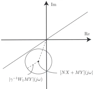
[NX+MY](jω)
|γ−1W
1MY|(jω)
Re Im
Fig. 1. Graphical illustration of nominal performance
2.2 Main Lemma
The main objective is to find a set of convex constraints
(with respect toX andY) to satisfy the control objective
in (6). The following lemma will be used in the proof of the main results of this paper:
Lemma 1. Suppose thatH(jω) =W1MY(NX+MY)−1 is the frequency response of a bounded analytic function in the right half plane. Then, (6) is met if and only if there
exists a stable proper rational transfer functionF(s) that
satisfies
Re{(NX+MY −γ−1|W1MY|)F(jω)}>0, ∀ω∈Ω
Proof : The basic idea is similar to that of the proof of Theorem 1 in Rantzer and Megretski [1994]. From Fig. 1, it is clear that (6) is satisfied if and only if the disk
of radius γ−1|W1MY| centered at NX +MY does not
include the origin for allω ∈Ω. This is equivalent to the
existence of a line passing through origin that does not
intersect the disk. Therefore, at every given frequency,ω,
there exists a complex numberf(jω) that can make rotate
the disk such that it lays inside the right hand side of the imaginary axis. Hence, we have
Re{(NX+MY −γ−1|W1MY|)f(jω)}>0 (7)
for allω∈Ω. In Rantzer and Megretski [1994], it is shown
that f(jω) can be approximated arbitrarily well by the
frequency response of a rational stable transfer function
F(s), if and only if
Z= (NX+MY −γ0−1|W1MY|)−1 (8)
is analytic in the right half plane for allγ0> γ. However,
(NX +MY)−1 is stable because of the stability of H.
On the other hand, by decreasing γ0 from infinity to γ,
the poles ofZ move continuously withγ0. Thus,Z is not
analytic in the right half plane if and only ifZ−1(jω) = 0
for a given frequency, which is not the case because the
disk shown in Fig. 1 does not include the origin. 2
2.3 Nominal and robust performance
The set of all controllers that meet the nominal perfor-mance defined by the weighted norm of sensitivity func-tions are given in the following theorem.
Theorem 1. Given the frequency response modelGin (1) and the frequency response of a bounded weighting filter
W1, the following statements are equivalent:
(a)There exists a controllerK that stabilizesGand
sup
ω∈Ω|W1(1 +GK)
−1|< γ (9)
(b)There existX, Y ∈RH∞withK=XY−1, such that
γ−1|W
1MY|(jω)< Re{[NX+MY](jω)}, ∀ω∈Ω
Proof :(b⇒a) SinceNX+MY is analytic in the right
half plane and its real part is positive for all ω ∈ Ω, it
will not turn around the origin when ω turns around the
Nyquist contour, so its inverse is stable and therefore K
stabilizesG. On the other hand, we have
|[NX+MY](jω)| ≥Re{[NX+MY](jω)}, ∀ω∈Ω
which leads to
|W1MY|(jω)< γ|NX+MY|(jω) ∀ω∈Ω
and consequently to (9) in Statement (a).
(a⇒b) Assume thatK=X0Y0−1 satisfies Statement (a)
but not Statement (b). Then, according to Lemma 1 there
exists a stable proper rational transfer functionF(s), such
that
Re{(NX0+MY0−γ−1|W1MY0|)F(jω)}>0 ∀ω∈Ω
Therefore, there exist X = X0F and Y = Y0F with
K=XY−1=X0Y0−1, such that Statement (b) hold. 2
This theorem can be applied straightforwardly to other sensitivity functions in (3)-(5).
The necessary and sufficient conditions for robust per-formance of closed-loop systems with frequency-domain uncertainty can be developed in the same way. Suppose that the frequency response of the plant model with some disk additive uncertainty is available as :
˜
N(jω) =N(jω) +|Wn(jω)|δnejθn (10) ˜
M(jω) =M(jω) +|Wm(jω)|δmejθm (11)
where |δn| ≤1, |δm| ≤ 1 andθn, θm ∈[0,2π]. This type
of models can be easily obtained by spectral analysis of
measured data, whereWnandWmare computed from the
covariance of the estimates for a given confidence interval (see Ljung [1999]).
If we consider the nominal performance as defined in (6), the robust performance condition becomes:
sup ω∈Ω
|W1MY|+|W1Wm|
|NX+MY| − |WnX| − |WmY| < γ (12)
Equivalently, at anyω∈Ω a disk of radius
r(ω) =γ−1|W1MY|+γ−1|W1Wm|+|WnX|+|WmY| (13)
centered at [NX+MY](jω) should not include the origin.
This can be presented as a set of convex constraints with
respect to X andY as follows:
r(ω)< Re{[NX+MY](jω)}, ∀ω∈Ω (14) 3. POLYTOPIC UNCERTAINTY
Another frequency-domain uncertainty is the polytopic uncertainty that covers multimodel uncertainty and para-metric uncertainty, as will be explained later, with some
approximation. In this type of uncertainty, the frequency response of the model is given as:
G(λ, jω) =N(λ, jω)M−1(λ, jω) (15) where N(λ, jω) = m i=1 λiNi(jω) (16) M(λ, jω) = m i=1 λiMi(jω) (17)
andλi ≥0,qi=1λi = 1 andλis the convex hull ofλis.
It can be shown that the following constraints
γ−1|W
1MiY|< Re{[NiX+MiY](jω)}, ∀ω∈Ω (18)
and for i = 1, . . . , m are sufficient conditions for robust
performance of the closed-loop system with polytopic uncertainty. It suffices to compute the convex combination of the constraints in (18) as γ−1m i=1 λi|W1MiY|< Re m i=1 λi[NiX+MiY] ,∀ω∈Ω Noting that: m i=1 λiW1MiY ≤ m i=1 λi|W1MiY| (19) we obtain: γ−1|W1M(λ)Y|< Re{N(λ)X+M(λ)Y](jω)}, ∀ω∈Ω
Then, according to Theorem 1 the upper bound for the
weighted sensitivity function is satisfied for allλ.
Remark:In a data-driven approach, a parametric model of the plant can be identified together with its parametric uncertainty using the classical prediction error methods (see Ljung [1999]). The parametric uncertainty is charac-terized by an ellipsoid in the parameter space and can be computed using the asymptotic covariance matrix of the parameters for a given probability level. This parametric uncertainty can be transferred into the frequency domain by a linear transformation, which is accurate enough for large data length. In the complex plane, this parametric uncertainty is represented by an ellipse at each frequency
and can be very well approximated with anm-side polygon
(m >2) of minimum area that circumscribes each ellipse. This way, the parametric uncertainty can be taken into account using the polytopic frequency-domain uncertainty with almost no conservatism.
Although the constraints for polytopic uncertainty are only sufficient, for some class of models and some sensi-tivity functions the necessary and sufficient conditions can be developed. The following theorem represents the results
for systems that have polytopic uncertainty only inN.
Theorem 2. Consider the frequency response model given
in (15) with N(λ, jω) in (16) and M(λ, jω) = M(jω).
Then, the following statements are equivalent:
(a)Controller KstabilizesG(λ) =N(λ)M−1,∀λand
sup
ω∈Ω|W1(1 +G(λ)K)
−1|< γ
(b)There existX, Y ∈RH∞such that K=XY−1, and
γ−1|W
1MY(jω)|< Re{[NiX+MY](jω)},∀ω∈Ω (20) and fori= 1, . . . , m.
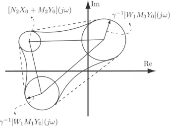
[N2X0+M2Y0](jω)
γ−1|W1M1Y0|(jω)
γ−1|W1M3Y0|(jω)
Re Im
Fig. 2. Graphical illustration of the constraints for poly-topic uncertainty with 3 vertices
Proof :(b⇒a) The convex combination of the constraints in (20) leads to
γ−1|W
1MY(jω)|< Re{[N(λ)X+MY](jω)} (21)
for all ω ∈ Ω and for all λ. So Statement (a) can be
concluded using the result of Theorem 1.
(a ⇒ b) Suppose that (a) is satisfied with the controller
K = X0Y0−1. Therefore, all disks of the same radius,
γ−1|W
1MY0|, centered inside a polygon created by the
m vertices, NiX0+MY0, do not include the origin. This
represents a convex set, which is the convex hull of the
m disks. Therefore, there exists always a line that passes
through the origin and does not intersect this convex set. As a result, similar to the proof of Lemma 1, there exists
a stable transfer functionF(s) such that:
Re{[NiX0+MY0−γ−1|W1MY0|]F(jω)}>0, ∀ω∈Ω
and for i = 1, . . . , m. Hence X = X0F and Y = Y0F
satisfies the inequalities in Statement (b). 2
Remark:Theorem 2 considers only the plant model with
polytopic uncertainty in N. This represents the class of
stable systems that may have some fixed poles on the imaginary axis. It covers also the unstable systems with
no uncertainty in M. A polytopic uncertainty in M will
change the radius of the disks centered atNiX0+MiY0,
such that the whole set of the disks will not be necessarily convex. Figure 2 shows a case in which the set of the disks is not convex but is inside the convex hull of the disks. This is always true because of the constraint in (19). In the special case shown in Fig. 2, we observe that the set of disks does not include the origin but the convex hull
does. Similarly, Statement (b) in Theorem 2 is a sufficient
condition for satisfying an upper bound on the weighted
sensitivity functions T or V, since the radius of the disks,
at each frequency, will not be constant for the whole polygon. However, it will be still necessary and sufficient
for an upper bound on the weighted sensitivity functionU
in (4).
4. FIXED-ORDER CONTROLLER DESIGN In this section we show how an optimal fixed-order con-troller can be designed for frequency-domain models by
convex optimization. For simplicity of presentation, we consider only the case without uncertainty. This problem is defined as: min X,Y γ subject to γ−1|W 1MY(jω)|< Re{[NX+MY](jω)},∀ω∈Ω (22) There are different practical and implementation issues in this optimization problem that will be discussed in this section. Note that the nonlinearity caused by the
multi-plication ofγ−1 and one of the optimization variables,Y,
can be easily solved by the iterative bisection algorithm.
4.1 Controller parameterization
A linear parameterization of X and Y keeps the
con-straints in (22) convex. As a result,X(s) andY(s) are
lin-early parameterized asX(s) =ρTxφ(s) andY(s) =ρTyφ(s), where ρTx = [ρx0· · ·ρxn] and ρTy = [1, ρy1· · ·ρyn] are the vectors of the controller parameters and
φT(s) = [1, φ
1(s)· · · , φn(s)] (23)
is a vector of stable orthogonal basis functions. A simple choice, is the Laguerre basis functions given by
φi(s) = √
2ξ(s−ξ)i−1 (s+ξ)i
with ξ >0 and i = 1,· · · , n. These basis functions have
only one parameter,ξ, to be selected.
4.2 Frequency response models
Finding the coprime factors of a given plant is a standard problem in control when the model of the plant is available (Zhou [1998]). For stable systems, a trivial choice is
N = G and M = 1. For unstable systems, in a
data-driven setting, a stabilizing controller is needed for data
acquisition purpose. In this case,N(jω) is the frequency
function between the reference signal and the measured
output, while M(jω) is the frequency function between
the reference signal and the plant input. It is evident
that in this case N(jω) and M(jω) are both stable and
N(jω)/M(jω) represents the frequency response of the
plant model. Although, the coprime factors are not unique for a given system, their choice has only an effect for low order controller design and this effect will be reduced by increasing the controller order.
4.3 Finite number of constraints
The constraints in (22) should be satisfied for all ω ∈Ω,
which is an infinite set. This problem is known as semi-infinite programming or robust optimization and there exist different methods to solve it. A very simple and practical solution to this problem is to choose a finite set of frequencies
Ωp={ω1, ω2,· · ·, ωp}
and satisfy the constraints for this set. This way, the problem is converted to a semi-definite programming that can be solved efficiently with the existing solvers.
Another solution is to use a randomized approach, in which the constraints are satisfied for a finite set of randomly
chosen frequencies. In this approach a bound on the violation probability of the constraints can be derived which goes to zero when the number of samples goes to infinity (see Calafiore and Campi [2006] and Alamo et al. [2010]). It should be mentioned that in a data-driven framework, the frequency domain uncertainties are given by some stochastic bounds. Therefore, even if the
constraints are met for allω, the stability, robustness and
performance are guaranteed with a probability level. As a result, the use of randomized method to solve the robust optimization problem in (22) is fully compatible with the uncertainty description of the frequency-domain model of the proposed approach.
4.4 Solution by linear programming
The convex constraints in (22) are equivalent to the following linear constraints:
Re{[NX+MY](jω)−γ−1ejθW1MY(jω)}>0, (24)
∀ω ∈ Ω and ∀θ ∈ [0,2π[. In fact, γ−1ejθW1MY(jω)
represents the circle in Fig. 1. Note that ejθ can be very
well approximated by a polygon of q > 2 vertices with
least area that circumscribes it. By gridding ω and over
bounding the circle ejθ, a finite set of linear constraints
will be obtained as follows:
Re [NX+MY](jωi)−γ−1 e j2πk/q cos(π/q)W1MY(jωi) >0 fori= 1, . . . , pandk= 1, . . . , q (25) Therefore, the convex constraints in (22) can be replaced
by the above p× q linear constraints and then γ can
be minimized by an iterative bisection algorithm. At each iteration a linear feasibility problem can be solved efficiently even if the number of constraints are large.
4.5 Experimental results
In this example, the experimental data are used to com-pute a robust controller with respect to frequency-domain uncertainty. An electro-mechanical flexible transmission system which consists of three disks connected by elastic belts is considered. The first disk is coupled to a servo motor which is derived by a current amplifier. The position of the third disk is measured with an incremental encoder and controlled by a proportional controller. The input of the system is the reference position for the third disk (see Fig. 3). This system is excited by a PRBS signal with a
sampling period ofT s= 40ms and the data length is 765.
Figure 4 shows the experimental data that are used to
identify a frequency domain model usingspacommand in
Identification toolbox of Matlab. The Nyquist diagram of this spectral model together with the uncertainty disks of 0.95 probability are given in Fig. 5. The uncertainty disks
are approximated by a polygon ofm= 20 vertices and the
goal is to design a stabilizing controller that minimizes γ
whereW1S∞< γ, withW1(z) =z−z−0.196.
In the proposed method, discrete-time Laguerre basis
functions of order 4 witha= 0 (FIR filter) are considered
forX andY. The resulting controller is
K(z) =20.3(z
2−1.88z+ 0.92)(z2−1.278z+ 0.6057)
(z+ 0.72)(z−1)(z2+ 0.209z+ 0.563) ,
drive disk load disk
speed reduction disk
Fig. 3. Flexible transmission system
0 5 10 15 20 25 30 −0.2 −0.1 0 0.1 0.2 Time (seconds) Position in rad y1 0 5 10 15 20 25 30 −0.2 −0.1 0 0.1 0.2 u1 Time (seconds) Position in rad
Fig. 4. Experimental identification data.
−3 −2 −1 0 1 2 3 −5 −4 −3 −2 −1 0 Real axis imaginary axis
Fig. 5. Nyquist diagram of the spectral model together with uncertainty disks
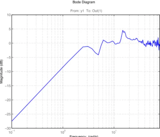
10−1 100 101 −30 −25 −20 −15 −10 −5 0 5 10
From: y1 To: Out(1)
Magnitude (dB)
Bode Diagram
Frequency (rad/s)
Fig. 6. Magnitude Bode diagram of the sensitivity function
which achieves an optimal performance of γ = 2.12.
Figure 6 shows the magnitude of the Bode diagram of the sensitivity function for the nominal model. It can be observed that the sensitivity function is small at low frequencies and its maximum value is less than 5db which guarantees a good stability margin.
5. CONCLUSIONS
In comparison with the classical model-based H∞
con-troller design the following features can be highlighted:
• Only frequency response of the plant is used for
controller design and no parametric model is required.
• Pure input/output time delay can be considered with
no approximation.
• Frequency-domain uncertainty is taken into account
with almost no conservatism.
• Parametric uncertainty in identified models with
noisy data can be considered in a stochastic sense with almost no conservatism.
• Fixed-order controllers can be designed with direct
optimization (no need for model or controller order reduction).
Clearly, the choice of basis functions affects the optimiza-tion results for low-order controllers. Their optimal choice and the extension of the results to multivariable systems are considered for future research works.
REFERENCES
T. Alamo, R. Tempo, and A. Luque. On the sample com-plexity of probabilistic analysis and design methods. In
Perspectives in Mathematical System Theory, Control, and Signal Processing, pages 39–55. Springer, 2010.
A. S. Bazanella, L. Campestrini, and D. Eckhard.
Data-driven Controller Design: The H2 Approach. Springer, 2012.
G. Calafiore and M. C. Campi. The scenario approach
to robust control design. IEEE Trans. on Automatic
Control, 51(5):742–753, May 2006.
M. C. Campi, A. Lecchini, and S. M. Savaresi. Virtual reference feedback tuning: A direct method for the
design of feedback controllers. Automatica, 38:1337–
1346, 2002.
A. J. Den Hamer, S. Weiland, and M. Steinbuch. Model-free norm-based fixed structure controller synthesis. In
48th IEEE Conference on Decision and Control, pages 4030–4035, Shanghai, China, 2009.
S. Formentin, K. Van Heusden, and A. Karimi. A compar-ison of model-based and data-driven controller tuning.
Int. Journal of Adaptive Control and Signal Processing, 2013. doi: 10.1002/acs.2415.
G. Galdos, A. Karimi, and R. Longchamp. H∞controller
design for spectral MIMO models by convex
optimiza-tion. Journal of Process Control, 20(10):1175 – 1182,
2010.
H. Hjalmarsson, M. Gevers, S. Gunnarsson, and O. Lequin. Iterative feedback tuning: Theory and application.
IEEE Control Systems Magazine, pages 26–41, 1998. R. Hoogendijk, A. J. Den Hamer, G. Angelis, R. van de
Molengraft, and M. Steinbuch. Frequency response data based optimal control using the data based symmetric
root locus. InIEEE Int. Conference on Control
Appli-cations, pages 257–262, Yokohama, Japan, 2010. L. C. Kammer, R. R. Bitmead, and P. L. Bartlett. Direct
iterative tuning via spectral analysis. Automatica, 36
(9):1301–1307, 2000.
A. Karimi. Frequency-domain robust control toolbox. In
52nd IEEE Conference in Decision and Control, pages 3744 – 3749, 2013.
A. Karimi and G. Galdos. Fixed-orderH∞ controller
de-sign for nonparametric models by convex optimization.
Automatica, 46(8):1388–1394, 2010.
A. Karimi, L. Miˇskovi´c, and D. Bonvin. Iterative
correlation-based controller tuning. Int. Journal of
Adaptive Control and Signal Processing, 18(8):645–664, 2004.
A. Karimi, M. Kunze, and R. Longchamp. Robust con-troller design by linear programming with application to
a double-axis positioning system. Control Engineering
Practice, 15(2):197–208, February 2007.
L. H. Keel and S. P. Bhattacharyya. Controller synthesis
free of analytical models: Three term controllers. IEEE
Trans. on Automatic Control, 53(6):1353–1369, July 2008.
S Khadraoui, HN Nounou, MN Nounou, A Datta, and
SP Bhattacharyya. A measurement-based approach
for designing reduced-order controllers with guaranteed
bounded error. Int. Journal of Control, 86(9):1586–
1596, 2013.
I. D. Landau, R. Lozano, M. M’Saad, and A. Karimi.
Adaptive Control: Algorithms, Analysis and Applica-tions. Springer-Verlag, London, 2011.
L. Ljung. System Identification - Theory for the User.
Prentice Hall, NJ, USA, second edition, 1999.
H. Parastvand and M. J. Khosrowjerdi. Controller
synthe-sis free of analytical model: fixed-order controllers. Int.
Journal of Systems Science, (ahead-of-print), 2014. A. Rantzer and A. Megretski. Convex parameterization
of robustly stabilizing controllers. IEEE Trans. on
Automatic Control, 39(9):1802–1808, September 1994. K. van Heusden, A. Karimi, and D. Bonvin. Data-driven
model reference control with asymptotically guaranteed
stability. Int. Journal of Adaptive Control and Signal
Processing, 25(4):331–351, 2011.
K. Zhou.Essentials of Robust Control. Prentice Hall, New