• No results found

Bayesian Change Point Analysis of Copy Number Variants Using Human Next Generation Sequencing Data

N/A
N/A
Protected

Academic year: 2021

Share "Bayesian Change Point Analysis of Copy Number Variants Using Human Next Generation Sequencing Data"

Copied!
148
0
0

Loading.... (view fulltext now)

Full text

(1)

BAYESIAN CHANGE POINT ANALYSIS of COPY NUMBER VARIANTS

USING HUMAN NEXT GENERATION SEQUENCING DATA

A DISSERTATION IN

Mathematics

and

Molecular Biology and Biolochemistry

Presented to the Faculty of the University

of Missouri-Kansas City in partial fulfillment of

the requirements for the degree

DOCTOR OF PHILOSOPHY

by

Jianfeng Meng

MS, University of Colorda Health Science Center, 2007

MS, Indiana University, 2001

MPH, Sichuan University HuaXi School of Public Health, 1991

MD, Sichuan University HaiXi Health Science Center, 1988

Kansas City, Missouri

2014

(2)

c

Jianfeng Meng

2014

All Rights Reserved

(3)

BAYESIAN CHANGE POINT ANALYSIS of COPY NUMBER VARIANTS

USING HUMAN NEXT GENERATION SEQUENCING DATA

Jianfeng Meng, Candidate for the Doctor of Philosophy Degree

University of Missouri-Kansas City, 2014

ABSTRACT

Read count analysis is the principal strategy implemented in detection of copy

num-ber variants using human next generation sequencing (NGS) data. Read count data

from NGS has been demonstrated to follow non homogeneous Poisson distributions.

The current change point analysis methods for detection of copy number variants are

based on normal distribution assumption and used ordinary normal approximation in

their algorithms. To improve sensitivity and reduce false positive rate for detection

of copy number variants, we developed three models: one Bayesian Anscombe

nor-mal approximation model for single genome, one Bayesian Poisson model for single

genome, and a Bayesian Anscome normal approximation model for paired genome.

The Bayesian statistics have been optimized for detection of change points and copy

numbers at single and multiple change points through Monte Carlo simulations. Three

R packages based on these models have been built up to simulate Poisson

distribu-tion data, estimate and display copy number variants in table and graphics. The high

sensitivity and specificity of these models have been demonstrated in simulated read

count data with known Poisson distribution and in human NGS read count data as

well in comparison to other popular packages.

(4)

APPROVAL PAGE

The faculty listed below, appointed by the Dean of Graduate Studies have

exam-ined a dissertation titled ”Bayesian Change Point Analysis of Copy Number Variants

Using Human Next Generation Sequencing Data”, presented by Jianfeng Meng,

can-didate for the DOCTOR OF PHILOSOPHY degree, and certify that in their opinion

it is worthy of acceptance.

Supervisory Committee

Jie Chen, Ph.D., Committee Chair

Department of Mathematics and Statistics

Shui Qing Ye, Ph.D.,

Department of Biomedical & Health Informatics

Gerald J Wyckoff, P.h.D,

Division of Molecular Biology and Biochemistry

Majid Bani-Yaghoub, P.h.D,

Department of Mathematics and Statistics

Xiao-qiang Yu, P.h.D,

(5)

CONTENTS

ABSTRACT

. . . .

iii

LIST OF ILLUSTRATIONS

. . . .

vii

LIST OF TABLES

. . . .

ix

ACKNOWLEDGEMENTS

. . . .

xi

Chapter

1. BACKGROUND

. . . .

1

1.1

Detection of CNVs . . . .

2

1.2

Detection of CNVs Using Next Generation Sequencing Data .

5

1.3

Change Point Data Analysis

. . . .

9

1.4

Bayesian Change Point Analysis . . . .

18

2. SINGLE GENOME BAYESIAN APPROACHES IN NGS

READ COUNT ANALYSIS

. . . .

21

2.1

The Models . . . .

21

2.2

Change Point Model Under Normal Transformation

. . . . .

22

2.2.1

Rationale . . . .

22

2.2.2

No Change Point Model

. . . .

23

2.2.3

One Change Point Model . . . .

28

2.2.4

H0

vs.

H1

and Change Point

. . . .

33

2.3

Bayesian Approach to Poisson Change Point Model . . . .

34

2.3.1

No Change Point Model (

H

0

) . . . .

35

2.3.2

One Change Point Model (

H

1

) . . . .

37

2.3.3

H

0

vs.

H

1

and Change Point

. . . .

40

2.4

Multiple Change Point Decomposition . . . .

42

2.5

Data . . . .

43

2.5.1

One Change Point Simulation Procedure . . . .

43

(6)

2.5.3

Next Generation Sequencing (NGS) Data Sets . . .

46

2.6

Evaluation . . . .

49

2.6.1

Definition

. . . .

49

2.6.2

Evaluation Indicies for One Change Point and

Mul-tiple Change Point Simulation Data . . . .

51

2.6.3

Evaluation Indices for NGS Data . . . .

55

2.7

Results . . . .

59

2.7.1

BayNormal . . . .

59

2.7.2

BayGamma

. . . .

68

2.7.3

Comparisons . . . .

79

2.8

Conclusion . . . .

85

3. NORMAL APPROXIMATION BATESIAN CHANGE POINT

MODEL FOR PAIRED GENOMES

. . . .

87

3.1

Rationale . . . .

87

3.2

Models . . . .

87

3.2.1

No Change Point Model

. . . .

89

3.2.2

One Change Point Model . . . .

93

3.2.3

H

0

vs.

H

1

and Change Point

. . . .

96

3.3

Multiple Change Point Decomposition . . . .

98

3.4

Data . . . .

98

3.4.1

One Change Point Read Count Data Simulation in

Paired Genomes . . . .

98

3.4.2

Multiple Change Point Data Simulation in Paired

Genomes . . . .

99

3.4.3

Next Generation Sequencing Datasets . . . .

100

3.5

Evaluation . . . .

101

3.5.1

Evaluation Indices for One Change Point and

Multi-ple Change Point Data . . . .

101

3.5.2

Evaluation Indices for NGS in Paired Genomes . . .

104

3.6

Results . . . .

108

3.6.1

PairedBayNormal . . . .

108

3.7

Conclusion . . . .

117

4. CONCLUSION AND FUTURE WORK

. . . .

121

4.1

Conclusion . . . .

121

4.2

Future Work . . . .

125

REFERENCES

. . . .

127

(7)

LIST OF ILLUSTRATIONS

Figure

Page

2.1

One Change Point Read Count Data Simulation

. . . .

45

2.2

Multiple Change Point Read Count Data Simulation

. . . .

47

2.3

Human NGS Read Count Data

. . . .

48

2.4

Human NGS Read Count Data Simulation

. . . .

50

2.5

LnOR

k

at Possible Single Change Points by BayNormal

. . . .

60

2.6

Impact of Window Size (or Segment Length) on ECP of mlnOR

by BayNormal

. . . .

62

2.7

Impact of The Assumed Change Point Location on ECP of mlnOR

by BayNormal

. . . .

63

2.8

Estimated Read Counts and Copy Numbers of Human NGS Read

Count Data By BayNorma

. . . .

69

2.9

Log Posterior Odds (

lnOR

k

) at Possible Change Points by BayGamma 71

2.10

Impact of Segment Length on ECP of mlnOR by BayGamma

. . .

72

2.11

Impact of Assumed Change Point Location on ECP of mlnOR by

BayGamma

. . . .

74

2.12

Histogram of Identified Change Points by BayNormal

. . . .

80

2.13

Histogram of Identified Change Points by BayGamma

. . . .

81

(8)

3.1

Log Posterior Odds Ratio (lnOR) by PairedBayNormal

. . . .

110

3.2

Adjusted Log Posterior Odds Ratio (∆ lnOR) by PairedBayNormal 111

3.3

Impact of Segment Length on ECP of m∆

lnOR

k

by

PairedBayNor-mal

. . . .

112

3.4

Impact of Change Point Location on ECP of m∆lnOR by

Paired-BayNormal

. . . .

113

(9)

LIST OF TABLES

Table

Page

2.1

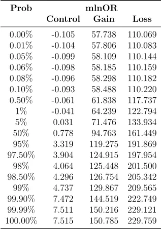
Empirical Cumulative Distribution of Maximum Log Posterior Odds

Ratio (mlnOR) by BayNormal

. . . .

64

2.2

Evaluation of Single Change Point Detection at OR.level=10.0 by

BayNormal

. . . .

66

2.3

Evaluation of Multiple Change Point Detection by BayNormal

. .

67

2.4

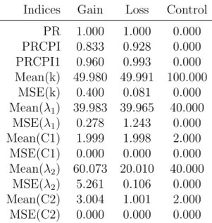
Evaluation on Human NGS+Simulation Data by BayNormal

. . .

68

2.5

Empirical Cumulative Distribution of Maximum Posterior Odds

(mlnOR) by BayGamma

. . . .

75

2.6

Evaluation of Single Change Point Detection at OR.level=10.0 by

BayGamma

. . . .

76

2.7

Evaluation of Multiple Change Point Detection By BayGamma

. .

77

2.8

Evaluation on Human NGS+Simulation Data by BayGamma

. . .

78

2.9

Evaluation of Single Change Point Detection by CBS

. . . .

83

2.10

Evaluation of Multiple Change Point Detection by CBS

. . . .

84

2.11

Evaluation on Human NGS+Simulation Data by CBS

. . . .

84

3.1

Empirical Cumulative Distribution of Maximum Posterior Odds

Ratio (m∆ lnOR) by Paired BayNormal

. . . .

114

3.2

Evaluation of Single Change Point Detection at OR.level=3.0 by

(10)

3.3

Evaluation of Multiple Change Point Detection by Paired BayNormal 118

(11)

ACKNOWLEDGEMENTS

I am very grateful to my mentor Dr. Jie Chen for her continuous support, patience

and excellent guidance through my PhD study. The comments and advices from

my supervisory committee members are really valuable for the preparation of this

dissertation and for my career development. I want to thank all of these who have

provide helps during my study. The support from my lovely family are always strong

and consistent. Without their support, I may not continue the efforts towards this

degree. Thanks to the people who made this dissertation possible, especially put

together a nice LATEX template for me to use.

(12)
(13)

Chapter 1

BACKGROUND

Genetic variations refer to the differences in the sequence of genetic

materi-als (DNA) in human genome among individumateri-als.

Genetic variations take many

forms ranging from large chromosomal anomalies (segmental aneuploidy) to single

nucleotide variant (Abecasis et al, 2012). Among them, structural variants (SV)

in-volve quantitative (e.g. copy number variants, indels) or positional (translocations)

or orientation (inversion) alterations of DNA sequence with multiple or segmental

nucleotides. Copy number variation refers to copy number differences in a segment

of DNA among individuals. Copy number variation is evidenced from either failure

to detect a certain DNA segment (deletion) or identification of multiple copies of a

DNA sequence (insertion) per haploid genome in comparison with reference human

genome sequence. A copy number variant (CNV) was usually defined as the

dupli-cation, insertion, or deletion of DNA segment larger than 1 kb. With the advent of

next-generating sequencing and new generation arrays, several studies used a

mini-mal length of 500bp to define the size of DNA segment for copy number variation

(Valsesia et al, 2013).

CNVs have been found genome wide in humans and other species. CNVs could

occur in both normal and disease population. The comparison of CNVs among

differ-ent human populations or across species has been explored to understand the genetic

diversity with the consequence of genetic evolution and disease susceptibility (Conrad

(14)

and Hurles, 2007). Some CNVs were likely to be associated with common diseases

(Craddock et al, 2010).

1.1

Detection of CNVs

Gross CNVs were initially detected by karyotyping in the early days of

cytoge-netic, where the number and structure of chromosomes in the sample of cells were

examined. In past decades, the evolution of CNV detection techniques from

Fluores-cent In Situ Hybridization (FISH) in early 1980 to new technology made it possible

to be more reliable, high throughput and fine resolution in the detection of CNVs

(Langer-Safter et al, 1982). The current widely used techniques include comparative

genome hybridization (CGH), single nucleotide polymorphism (SNP) array and next

generation sequencing based methods.

CGH is developed based on the assumption that CNVs can be detected by the

relative ratio of the test sample DNA amounts to the reference genome DNA. The

flu-orescence labeled test and reference DNA in ratio 1:1 were simultaneously hybridized

to a normal metaphase spread of chromosomes or a DNA microarray (aCGH), and

bind competitively at the locus of the origin. If there are more copies of test DNA

than the reference DNA, a relatively higher intensity of the test sample color in a

specific chromosomal region will be captured through fluorescence microscope and

computer software. Conversely, a relative lower intensity of the test sample color in

comparison to the reference DNA color will indicate the loss of DNA sequence copies

in the test samples (Ren et al, 2005; Urban et al, 2006). The location of copy number

will be determined by known DNA sequences embedded on the DNA microarray.

SNP array was originally used to detect single nucleotide polymorphisms (SNPs)

and to genotype human DNA in populations. The common procedure for SNP array

is that the test and reference sample DNA are hybridized to an DNA array

contain-ing hundreds of thousands even millions of unique nucleotide probe sequences with

(15)

fluorescent which is designed to bind complementarily to a target DNA subsequence.

Various computation algorithms have been implemented in converting the raw signals

into inferences about the presence or absence of each of the two alleles in different

platforms. Meanwhile, the probe signal intensity level either from summarization of

multiple SNP probe intensity or from singleton non-polymorphic probes incorporated

with genotype information is converted into single measure of row copy number by

comparing to that from a panel of reference samples (LaFramboise, 2009). Since SNP

array is relatively cheap to genotype individuals for previously known variants, it is

popularly used in population genetic studies to identify the association of SNPs and

copy number variations with disease traits (Valsesia et al, 2012). Dozens of statistical

methods have been developed to infer chromosomal segments of locally constant copy

number from the noisy raw copy number measurements. The algorithms range from

mainly Hidden Markov Model (HMM) and circular binary segmentation to mixture

models, maximum likelihood, regression, wavelet and genetic models (Lai et al, 2005;

Wang et al, 2007; Colella et al, 2007; Chen et al, 2009). However, considerable

varia-tions in sensitivity and specificity for identifying CNV boundary and determining the

number of CNVs called exist among programs. The CNV length, frequency of CNV

and features of CNV e.g. deletions or duplication in addition to SNP array platform

with density of selected SNPs may contribute to the accuracy of the detection across

multiple programs (Zhang et al, 2011).

DNA sequencing is a process of determining the precise order of nucleotides (A, G,

C and T) in a strand of DNA. Early DNA sequencing techniques is based on inferring

DNA sequences from differentiating labeled DNA fragments in DNA synthesis process

either through radiolabelled DNA and chemical cleavage of specific base (Maxam and

Gilbert, 1977) or through fluorescence labeled chain-termination inhibitor of DNA

polymerase. The high demand for low cost and fast sequencing has driven the

de-velopment of high throughput sequencing or next generation sequencing (NGS) in

(16)

which parallelized sequencing process produces thousands or millions of sequencing

reads simultaneously. Several platforms have been developed since the mid 1990s.

Among them, 454 Pyrosequencing by Roche Diagnostic, Applied SOLiD technology

and Illumina (Solexa) sequencing are the most popularly used. As an example to

illus-trate the next generation sequencing technique, Illumina Solexa sequencing system is

based on reversible dye terminators technology. In this method, DNA fragment with

primers are attached to solid surfaces and amplified by PCR so that DNA clusters of

clonal DNA are formed. To determine the sequence, four types of reversible

termina-tor nucleotides are added and non-incorporating nucleotides are washed away. After

a camera takes the fluorescent image, the dye and 3 blockers are chemically removed

so that the next cycling can begin. The DNA chains are extended one nucleotide at

one time and an image is acquired sequentially until a DNA sequence is completed.

By combined with massively parallelized sequencing technology, very large arrays of

DNA colonies can be sequenced concurrently (Margulies et al, 2005). Up to billions of

nucleotide reads per run within 1 to 10 days can be generated using Illumina

sequenc-ing system. In deep sequencsequenc-ing, total length of DNA sequences generated is many

times larger than the length of the sequence under the study due to the depth of the

process. Depth of coverage in massively paralleling sequencing refers to the number

of times a nucleotide is read during the sequencing process. More NGS methods are

under development. The extension of single read sequencing (also called single end

sequencing) to paired end reads or mate pairs (also called paired end sequencing)

offers additional information to detect copy number variation and other structural

variations such as inversion and translocation (Raphael et al, 2012; Medvedev et al,

2009). The comparison of NGS methods can be found in the excellent reviews by

Quail et al (2012) and Liu et al (2012). Since significant reduction in cost has been

achieved, the application of NGS has been used to sequence whole genome sequence

of thousand human individuals.

(17)

Compared to array based techniques, copy number analysis by NGS allows the

breakpoints of copy number regions to be determined more precisely because it does

not rely on predefined probes (Chiang and McCarroll, 2009). It also allows

detec-tion of smaller copy number variadetec-tions by simply increasing the depth of sequencing

(Chiang and McCarroll, 2009). Estimation of integer copy numbers from NGS data

is more accurate at high copy counts, since depths of coverage scale linearly with

copy number and it does not suffer from hybridization saturation (Alkan et al, 2009).

More and new allele specific copy numbers may be estimated from sequencing data,

while array-based techniques are restricted to predefined alleles. Allele specific copy

numbers are of interest because the functional alleles may be mutants leading to

dis-ease development (Stratton et al, 2009; Klambauer et al, 2012). Overall, NGS has

demonstrated higher sensitivity, in terms of types and sizes of variants that can be

detected.

1.2

Detection of CNVs Using Next Generation Sequencing Data

Strategy

The commonly used strategies include read depth analysis, paired end

mapping, split read approach, sequence assembly and combination algorithms. Read

depth analysis and sequence assembly can be applied on single end sequencing, while

paired end mapping and split read approach mainly depend on paired end sequencing

(PES) (Alkan et al, 2011; Valsesia et al, 2013; Teo et al, 2012).

Paired end mapping (PEM)

requires sequencing both ends (also called paired end

reads or mate pairs) of a genomic fragment of known size and then mapping the

end sequence pair to a reference sequence (Raphael et al, 2012). Since the distance

between paired end reads is expected to fall in fixed range, fragments overlapping

structural variant events in a test genome may result in discordant paired end

se-quences that map to different parts of the reference genome. Discordant paired ends

in length or direction indicate respectively possible indels or inversions or locations

(18)

(Medvedev et al, 2009). When sequenced ends of the fragment map to the reference

at a distance longer than expected, it is indicative of an insertion in the studied

genome. Vice versa, when sequenced ends of the fragment map to the reference at a

distance shorter than expected, it is indicative of a deletion in the studied genome.

As an example, if two ends of a fragment are mapped with a wrong orientation, it

could be an indication of an inversion. Several analysis tools based on detection of

discordant end-pairs and clustering of end pairs have been developed and used for

the estimate of SVs and CNVs (Koboldt et al, 2012). Paired end mapping is more

specific when lining back to genome resulting from two paired end reads compared

to single end mapping. Precise breakpoints can be determined through paired end

mapping. In addition to CNV, other SVs can be measured through it. However, the

detection resolution is limited to the distance between pairs, neither large nor very

small rearrangements can be detected, with the exception of large deletions (Valsesia

et al, 2013).

The split read (SR)

approach was used to detect deletion and insertion events when

one of paired end reads mapped uniquely onto a reference genome but the other one

of paired end reads can’t be mapped. It is assumed in the split read approach that the

unmapped read occurs because the breakpoints of deletion or insertion are inside the

reads in test genome. Therefore the analysis strategy is that the mapped end read is

taken as anchor point and the unmapped read can be mapped to reference genome by

splitting it into two fragments or three fragments. If two fragments are mapped to the

reference genome uniquely, it indicates deletion. If two ends of three fragments are

mapped to the reference genome uniquely, it indicates an insertion of middle part of

the unmapped end read (Ye et al, 2009). Identification of breakpoints with a pattern

growth algorithm was applied in the split read analysis (Ye et al, 2009).

De novo assembly

aligns a test genome sequence utilizing high sequencing depth

data. Then the sequence is compared to the reference sequence for detection of

(19)

dele-tions and inserdele-tions. The advantage is that different size of deledele-tions and inserdele-tions

even smaller than paired end insert size can be detected. However, de novo assembly

is very difficult for repeat rich regions and until recently was only possible with high

read depth (Iqbal et al, 2012; Simpson and Durbin, 2012).

Read depth

also called

read count (RC) analysis

is based on depth of

cover-age (DOC) in the NGS. It assumed that the sequencing process is uniform across a

genome and number of reads mapping to a region is expected to be proportional to

number of times the region appear in the DNA sample. A region that has deletion

(or duplication) is expected to have less (or more) reads mapping to it (Chiang and

McCarroll, 2009; Medvedev et al, 2009).

Read Count Analysis

Read count analysis are still the main strategy in analysis

of read data for copy number variations from both paired and single end sequencing

in literatures. After RC analysis was first used by Campbell (Campbell et al, 2008)

and Chiang (Chiang and McCarroll, 2009) to detect CNVs, several RC analysis

pack-ages have been developed to look for copy number difference in normal and diseased

populations (Yoon et al, 2009; Xie et al, 2009; Ivakno et al, 2010; Kim et al, 2010;

Xi et al, 2011). The analysis pipeline implemented in current packages for

discov-ering CNVs is conceptually derived from aCGH data analysis and can be divided

into four fundamental steps: read data filtering and sequence alignment; assignment

to bin/window; CNV region identification (segmentation); Copy number estimation

(Magi et al, 2012). Since the mappability of reads onto the reference genome sequence

influences the accuracy of read counts assignment, mappability correction has been

often applied. GC content in genome sequence and sequencing error among DNA

samples have been demonstrated to influence the accuracy of read generation in next

generation sequencing technology. Therefore GC content correction and sample

nor-malization are frequently seen in analysis packages.

(20)

vari-ation. Taking consideration of NGS read data from single genome, paired genomes

or multiple genomes three different strategies have been implemented. Various

al-gorithms have been developed for the segmentation process in each strategy. The

packages for single genome rely mostly on read depth data that are sequenced from

one single person, and sometimes integrated with read pair and read split information.

The packages for paired genomes are based on ratio or comparison between targeted

individual sequence data and a reference sequence data. A typical example is the

detection of CNVs in cancer patients compared with normal tissue or with a control

subject. Population based methods utilize read depth data from multiple samples.

Copy number estimation

The copy number calling algorithms are based on

seg-mentation and generate results about gain or loss of copy number or rough copy

numbers. The copy number of each event was inferred in RDxplorer (Yoon et al,

2009) by rounding the average normalized read counts in each individual to the

near-est integer. The normalized read counts is defined as 2 X (read count)/(mean read

count over the genome). The segments identified in ReadDepth by Miller et al (2011)

were called gains or losses if their mean value exceeded 1.5 standard deviation from the

mean probe value. The CNV calling for duplication or deletion in CNVnator (Abyzov

et al, 2009) is based on statistical significance t tests with multiple correction p value

in comparison with genomic average RD signal. ERDS by Zhu et al (2012) generates

initial copy number inference using continuous paired Hidden Markov Model (HMM)

for both deletion and duplication based on expected RD data in nonoverlaping

win-dows and refines the deletion and breakpoints of putative deletions by integrating

paired end mapping (PEM) and soft-clipping signatures to filter false positive and

confirm weak RD signals.

The copy number change based on read count ratio between test and control

samples is considered as gain or loss while segmentation algorithms for significantly

changed ratio along the genome position are applied (Chiang and McCarroll, 2009;

(21)

Xie et al, 2009; Kim et al, 2010; Ivakno et al, 2010; Xi et al, 2011).

Read count analysis requires that reads from sample DNA are mapped to the

reference genome sequence. Since reads from a novel sequence can’t be mapped to the

reference genome sequence, it is unable to detect a new insertion of DNA sequence

through read count analysis. Unlike PEM insertion signatures, RC analysis can’t

detect other SVs such as inversion or translocation. Furthermore uniquely mapping

reads to high repeat rich region is very difficult. These deteriorate the accuracy of RC

analysis in amounts and location of CNVs. To overcome the limitation of algorithm

only based on DOC, more packages applied combination algorithm with information

from DOC, PEM and SR as well as other features of sequence data at population

level for more accurate detection of CNVs (Medvedev et al, 2010; Miller et al, 2011;

Abyzov et al, 2009; Zhu et al, 2012; Klambauer et al, 2012; Bellos et al, 2009).

Overall, Most of these methods showed less sensitive and high false discovery

rate (

20% or more) in read datasets. Those may lead to wrong conclusions for

identification of disease variants in genetic association studies. Identifying factors

that may impact the accuracy of those methods and developing more sensitive and

accurate statistical methods with innovative strategy are crucial to improve CNV

detection using next generation sequencing technology. Since the segmentation plays

a crucial role in determining the copy number change, an improved algorithm is

expected to increase the sensitivity and reduce false positive rate in the detection.

The change point analysis is among one of these approaches. In the following section,

the detailed algorithm and mathematical deduction with respect to change point

analysis are illustrated so that improvements can be specified.

1.3

Change Point Data Analysis

Change Point Analysis

The change point problem refers to the identification

(22)

locations. Usually statistical inference about change points has two aspects. The

first is to detect if there is any change in the sequence of observed random variables.

The second is to estimate the number of changes and their corresponding locations.

The detection of CNVs along the human genome is actually a change point issue

where read counts change in bins corresponding to copy number change. This has

been recognized and applied in CNV detection packages.

Let

X

1

,

X

2

,

· · ·

,

X

n

be a sequence of independent random vectors (variables) with

probability distribution functions

F

1

,

F

2

,

· · ·

,

F

n

, respectively. Then in general, the

change point problem is to test the following null hypothesis,

H

0

:

F

1

=

F

2

=

· · ·

=

F

n

versus the alternative:

H

1

:

F1

=

· · ·

=

Fk

1

6

=

Fk

1

+1

=

· · ·

=

Fk

2

6

=

Fk

2

+1

=

· · ·

=

F

kq

6

=

F

kq+1

· · ·

=

F

n

where 1

< k

1

< k

2

<

· · ·

< k

q

< n

, q is the unknown number of change points

and

k

1

, k

2

,

· · ·

, k

q

are the respective unknown positions that have to be estimated. If

the distributions

F

1,

F

2,

· · ·

,

F

n

belong to a common parametric family

F

(

θ

), where

θ

R

p

, then the change point problem is to test the null hypothesis about the

population parameters

θ

i

, i

= 1

,

· · ·

, n

:

H

0

:

θ

1

=

θ

2

=

· · ·

=

θ

n

=

θ

(

unknown

)

(1.1)

(23)

H

1

:

θ

1

=

· · ·

=

θ

k

1

6

=

θ

k

1

+1

=

· · ·

=

θ

k

2

6

=

θ

k

2

+1

=

· · ·

=

θ

kq

6

=

θ

kq

+1

· · ·

=

θ

n

(1.2)

where q and

k

1

, k

2

,

· · ·

, k

q

have to be estimated. These hypotheses together reveal

the aspects of change point inference: determining if any change point exists in the

process and estimating the number and positions of change point(s).

The frequently used methods for change point inference in the literature are the

maximum likelihood ratio test, Bayesian test, nonparametric test, stochastic process,

information theoretic approach, and so on. Many of them can be found in a book by

Chen and Gupta (2012). Most of the change point studies were concentrated on the

case of a single change point in the random sequence. The problem of multiple change

points were rarely addressed by many authors. A binary segmentation procedure

(BSP) proposed by Vostrikova (1981) has been proved to be consistent and been

widely used in detecting multiple change points, and it has the merits of detecting

the number of change points and their positions simultaneously and saving a lot of

computation time. Briefly in the case we described in equation (1) and (2), several

steps are generally involved in the final identification of multiple change points. The

first step is to test for no change point versus one change point; that is, test the null

hypothesis by equation (1) versus the following alternative.

H

1

:

θ

1

=

· · ·

=

θ

k

6

=

θ

k+1

· · ·

=

θ

n

(1.3)

where k is the location of the single change point at this stage. If

H

0

is not

(24)

point and we go to step 2.

In step 2, the two subsequences before and after the change point found in step

1 are tested separately for a change. This process is repeated until no further

subse-quences have change points. The collection of change point locations found by above

steps is denoted by

{

k

ˆ

1

,

k

ˆ

2

,

· · ·

,

k

ˆ

q

}

, and the estimated total number of change points

is then q.

The majority of the models proposed for change point problems in the literatures

are the normal models (univariate or multivariate), perhaps due to the fact that the

normal model is the most common model in practice. These have been addressed by

Chen and Gupta (2012). Meanwhile, the gamma and exponential model, regression

model, hazard function model, binomial model, Poisson model as well as well smooth

and abrupt model have been reported in the literatures.

Application of Change Point Analysis in CNVs Detection

The copy

num-ber detection in aCGH experiments is based on the ratio of test sample intensity to

the reference sample intensity. Let

T

i

denote the test sample intensity at locus i on the

genome and

Ri

denotes the the corresponding reference sample intensity. The

normal-ized log base 2 ratio of the sample and reference intensities,

log

2

T

i

/R

i

, is considered

as a random variable used for the derivation of copy number. Here,

log

2

T

i

/R

i

= 0

indicates no DNA copy number change at locus i,

log

2

T

i

/R

i

<

0 reveals a deletion at

locus i, and

log

2

T

i

/R

i

>

0 signifies duplication in the test sample at that locus. This

random variable is assumed to follow a Gaussian distribution of mean 0 and constant

variance

σ

2

. Then, deviations from the constant parameters (mean and variance)

presented in

log2Ti/Ri

data may indicate a copy number change.

Among the many methods used for a CGH data, Olshen et al (2004) proposed a

circular binary segmentation (CBS) method to identify DNA copy number changes in

an aCGH database on the mean change point model. This CBS method is mainly the

combination of the likelihood ratio based test (Sen and Srivastava, 1975) for testing no

(25)

change in the mean against exactly one change in the mean with the BSP (Vestrikova,

1981) for searching multiple change points in the mean, assuming that the variance

is unchanged.

To illustrate the CBS algorithm, let

X

i

denote the normalized

log

2

T

i

/R

i

at the ith

locus along the chromosome;then

{X

i

}

is considered as a sequence of normal random

variables taken from

N

(

µ

i

, σ

i

2

), respectively, for

i

= 1

,

· · ·

, n

. Consider any segment

of the sequence of the log ratio intensities

X

i

to be spliced at the two ends to form a

circle;

Z

ij

, the likelihood ratio test statistic given by Sen and Srivastava (1975a) for

testing the hypothesis that they are from i+1 to j and its complement have different

means, is given by:

Zij

=

1

{

1

/

(

j

i

) + 1

/

(

n

j

+ 1)

}

12

{

S

j

S

i

j

i

S

n

S

j

+

S

i

n

j

+

i

}

(1.4)

with

Si

=

X1

+

X2

+

· · ·

+

Xi,

1

i < j

n.

The test statistic

Z

c

of the CBS is based on the modified likelihood-ratio test and

is given by:

Z

c

= max

1

i<j

n

|Z

ij

|

(1.5)

Z

c

allows for both a single change (j=n) and the epidemic alternative (

j < n

).

A change is claimed if the statistic exceeds an appropriate critical value at a given

significant level based on the null distribution. However, the null distribution of the

test statistic

Z

c

is not attainable so far in the literature of change point analysis.

(26)

Monte Carlo simulations or the approximation given by Segmund (1986) for the tail

probability when

X

i

s are normal. Once the null hypothesis of no change is rejected,

the change points are estimated to be i (and j) such that

Z

c

=

|Z

ij

|

and the procedure

is applied recursively to identify all the changes in the whole sequence of the log ratio

intensities of a chromosome.

Since the p-value given by the CBS for a specific locus being a change point,

however, is obtained by a permutation method and the calculation of such a p-value

takes a long computation time when the sequence is long, which is the case for high

density array data. The original R package was found to be the slowest computation

method by Pichard et al (2005). By modifying the analytic formula, an updated

version DNA copy (Venkatraman and Olshen, 2007) has improved the computational

speed of CBS. The DNA copy package has been widely used in copy number analysis

of aCGH data. Miller et al (2011) has applied CBS in the package ReadDepth for

analysis of CNV from NGS read counts which has been considered as one of the best

packages until now.

Change Point Analysis in NGS

Among single genome based approaches, Yoon

et al (2009) applied the event-wise testing (EWT) algorithm to define the region with

read count changes. Based on standardized read data counted in 100bp windows over

whole genome, the events for increased or reduced read depth data are identified by

upper or lower tail probability of approximated normal distribution in EWT. A

du-plication or deletion segment within consecutive windows is defined if the maximum

of the p values is lower than multiple corrected false positive rate (FPR). Miller et

al (2011) used normalized read count data in the package ReadDepth and adopted

circular binary segment algorithm which are widely used in aCGH data copy

num-ber estimation to identify the boundaries of the segment with read count changes.

CNVnator by Abyzov et al (2009) is based on combining the established mean shift

approach with additional multiple bandwidth partitioning approach. The mean shift

(27)

process is an iterative procedure that shifts each data points to the density maxim

along the mean shift vector, a gradient of probability density function. Boundaries of

genomic segments are identified by finding the consecutive pairs of bins with

mean-shift vectors switching direction. Iterative read depth signaling merging,

segmenta-tion and boundary identificasegmenta-tion are through greedy algorithm and significance tests.

FreeC by Boeva et al (2011) adopted LASSO based algorithms for segmentation of

normalized read count data. All these algorithms are based on normal approximation

of read counts data which may not reflect the true discrete data distribution.

In the early algorithms that utilize ratio of read counts between tumor and

con-trol samples, Segseq (Chiang and McCarroll, 2009) is a hybrid of local change point

analysis with a subsequent merging procedure that joints adjacent chromosomal

seg-ments. It partitions the genome into windows of fixed size, estimates the test-control

ratios for each window and merges the adjacent bins based on significance p value

threshold. CNV-seq by Xie et al (2009) transforms the read count ratio of Gaussian

variables to a t variable and calls copy number change based on p-value calculation

from greater or less than ratio 1 with optimized window size. rSW-seq (Kim et al,

2010) applies a recursive smith waterman algorithm to sequence reads from tumor

and matched control genomes that are combined and sorted in a no decreasing

or-der according to their genomic position and weighted differently for tumor (Wt) and

control (Wc). A large local positive (or negative) cumulative sum of weighted values

indicates a local copy number gain (or loss). For copy number gains, the algorithm

searches for the segment such that the partial cumulative sum is maximized and

iterated until no more alteration can be found. In package CNAseg, Ivakno et al

(2010) transferred the read count difference between tumor and control samples in

non-overlapping windows to hidden states of copy number using k-mean clustering

algorithm. Merging segments with the same copy number states is based on Pearson

(28)

table. The merging threshold is derived from flow cell splitting approach. BIC-seq

developed by Xi et al (2011) applied minimizing Bayesian information criterion (BIC)

on likelihood of mapped reads from tumor or control in reference genome positions

to define optimized breakpoints for segmentation. BIC-seq level function (B, t,

λ

)

(given a list of bins B, consecutive t bins in a window, and a tuning parameter for

smooth penalty) is iteratively evaluated until all windows with negative BIC-diff are

exhausted. False positives was identified by BIC-seq from the re-sampled data pulled

from a pool of tumor and control reads.

Poisson distribution of Read Counts

All of the above approaches are based on the

assumption of normal distribution or approximation of normal distribution. Actually

it has been demonstrated that read counts follows Poisson distribution. Under the

assumption that the reads are randomly and independently sampled from any location

of the test genome with equal probability, Bentley et al (2008) and Yoon et al (2009)

have reported that RCs by Illumina GA follow a Poisson distribution with a slight

over dispersion. The distribution of RC counts in fixed bin size window seems to be

more dispersed in data from Illumina and SOLiD than that from Roche. Smaller bin

size (e.g. 1000 bp compared to 2000 bp and 5000 bp) seems to have a more narrowly

distribution. Except Poisson distribution, negative binomial distribution seems to fit

the data more likely than Poisson distribution (Magi et al, 2012).

The over dispersion of RC data distribution can be accounted for by three main

reasons: the existence of genomic regions of duplications and deletions (CNVs); the

correlation between read coverage and the DNA local GC content; the correlation

between the read coverage and the mappability (i.e. the inability to map reads into

repetitive regions of the genome (Magi et al, 2012). It is estimated that the fraction

of a genome subject to variation of copy number is 3.7

7.0% (Conrad et al, 2010). It

was observed by Magi et al (2012) that the removal of genomic regions with known

CNVs reduces the index of dispersion of RC data distribution in either of Illumina,

(29)

SOLiD and Roche platforms and also in either of low and high coverage data. These

indicate that the existence of genomic regions of duplications and deletions (CNVs) is

the major reason for over dispersion of the data distribution especially after correction

of GC content and mappability error while the majority of RC data follow a Poisson

distribution with global average number of reads as its mean.

It was also noted that in RD data, the variance is lowest for deletion states (zero or

one copy) and variance increases proportionally with increasing copy number

(Bent-ley et al, 2008; Yoon et al, 2009). This observation is consistent with the Poisson

distribution in which the variance is equal to the average mean value. This differs

from the characteristic data from microarray CGH data in which variance in probe

ratios is lowest for the normal state (two copies) and probe variance increase from

copy number changes in both directions (Yoon et al, 2009).

By reducing the bin size to 100 bp, Yoon et al (2009) used normal distribution to

approximate standardized RD data. It has been noted by Olshen et al (2004) in copy

number detection using aCGH array that centering log ratio intensities around zero

for normalization of data to correct for confounding factors makes the copy numbers

unidentifiable without some additional modeling. For example, the normalized data

from diploid and triploid samples will appear similar. Miller et al (2011) recommended

a model of negative binomial distribution to approximate the over dispersed Poisson

distribution. As we know, a mixture of Poisson distributions with mean parameter

value

λ

which is drawn from a gamma distribution with shape parameter

α

and scale

parameter

β

follows a negative binomial distribution. Miller et al (2011) developed

a model of negative binomial distribution with

λ

as the median value of the Poisson

distribution and with

γ

as a variance parameter for

λ

from a gamma distribution.

Introduction of

γ

alters the variancemean ratio (VMR) and accounts for the excessive

variance from the over dispersion. The resulting root mean square error is three times

smaller than that of Poisson.

(30)

As illustrated above, read counts from NGS follows overdispersed Poisson

distri-bution in which the copy number variants seem to be the main reason accounting for

the overdispersion. Under the assumption of unchanged copy number variants, read

counts more likely follow homogeneous Poisson distribution. Therefore, the

identifi-cation of copy number variants is an issue to find change of Poisson distributions for

read counts data along the reference genome sequence.

1.4

Bayesian Change Point Analysis

It has long been recognized that Bayesian methods are well suited to find change

points (Smith, 1975; Worsley et al, 1986). Bayesian change point methods are based

on Bayesian inference according to Bayes’ rule. The posterior probability (

π

(

θ|X

)

is derived as a consequence of two antecedants, a prior probability (

π

0

(

θ

)) and a

likelihood function (L(

θ, X

) derived from a probability model for the data to be

observed.

π

(

θ|X

) =

L

(

θ, X

)

π

0

(

θ

)

m

(

X

)

(1.6)

where m(

X

) is the marginal likelihood of observed values and is same for all

hypotheses and often canceled in the relative posterior odds between two hypotheses.

All inferences are based on posterior distribution of

θ

.

Under null hypothesis (equation (1.1)), the integration of the product of prior

dis-tribution and likelihood function will generate the posterior probability of hypothesis

H

0

:

π

0

(

X

) =

P

(

θ


0

|X

). Under alternative hypothesis, that will generate the

posterior probability of

H

1

:

π

1

(

X

) =

p

(

θ


c

0

|X

). Bayesian factor which is the

ratio of integrated posterior probability of

θ

is preferred to be used for comparison

of multiple models by hypothesis testing. With specific k change point in mind, the

posterior probability of change point at k is:

π

1

(

k|X

) =

p

(

θ


c

0

(

k

)

|X

) is frequently

(31)

of posterior probabilities of the hypotheses given observed data.

OR

k

=

π

1

(

k|X

)

π

0

(

X

)

=

R

θ


c0

L

1

(

θ, k, X

)

π

0

(

θ


c

0

)

π

0

(

k

)

R

θ


0

L0

(

θ, X

)

π0

(

θ


0

)

(1.7)

The posterior odds

OR

k

is used to in this research for comparison of one change

point model at k vs

H0

. The threshold level will be derived from empirical distribution

of the posterior odds in Monte Carlo simulations.

Bayesian inference is used to update the probability estimate for a hypothesis as

additional evidence is acquired. If the evidence does not match up with a hypothesis,

one should reject the hypothesis. But if a hypothesis is extremely unlikely a prior,

one should also reject it, even if the evidence does not appear to match up. When the

prior distribution is uninformative, the Bayesian is just like a likelihood ratio test.

Bayesian utilized all information in the inferences including both the observed data

and prior belief for the parameters. Wald and Wolfowitz (1950) proved that every

Bayesian procedure is admissible. Under some conditions, all admissible procedures

are either Bayesian procedures or limits of Bayesian procedures (in various senses) in

decision theory.

Bayesian methods are very popular in change point analysis. Bayesian analysis

of Poisson data similar in spirit to the present work include Raftery and Akman

(1986); Gregory and Loredo (1992); West and Ogden (1997); Scargle (1998). However,

no Poisson Bayesian model has ever been used in CNV detection esp using next

generation sequencing data as we know. The application of Bayesian approaches in

big data as that from NGS is also challenging.

In present work, we developed a Bayesian change point model for single genome

and a Bayesian change point model for paired genomes based on Anscombe normal

(32)

approximation algorithm, and modified a Bayesian Poisson change point model to

identify the change points and estimate copy number variants from NGS read count

data in single genome. The statistics have been optimized for the detection of change

points and copy numbers at single and multiple change points. Three rapid R packages

have been developed to simulate Poisson data, estimate and display copy number

variants in table and graphics. The sensitivity and specificity are evaluated in both

simulated read count data with known Poisson distribution and in human NGS read

count in comparison to other popular packages.

(33)

Chapter 2

SINGLE GENOME BAYESIAN APPROACHES IN NGS READ

COUNT ANALYSIS

2.1

The Models

A reference human genome sequence (or a specific chromosome) with total g

nucleotides is divided into total n evenly spaced intervals with each interval having

b base pairs (called bin size). The next generation sequencing will produce total T

reads and each read has average

l

nucleotides called read length. The average read

counts per bin is equal to T/n.

Let

Xi

represents read counts in evenly spaced intervals i with bin size b bps,

where

X

i

= 0

,

1

, . . .

and

i

(1

,

2

,

· · ·

, n

) along the studied genome sequence and

n=int(g/b). We assume

X

i

follow independent Poisson distributions:

X

i

P ois

(

λ

i

)

with intensity parameter 0

λ

i

<

. Statistical inference for multiple change point

analysis is based on the following hypotheses testing. The nulll hypothesis is given by :

(34)

versus alternative hypothesis

H

1

:

λ

1

=

· · ·

=

λ

k

1

6

=

λ

k

1

+1

=

· · ·

=

λ

k

2

6

=

λ

k

2

+1

=

· · ·

=

λ

kq

6

=

λ

kq

+1

=

· · ·

=

λ

n

(2.2)

Under null hypothesis, all read counts follow identically independent Poisson

dis-tribution (i.e. there is no CNV in the genome segment) with parameter

λ

over the

seg-ment, while under alternative hypothesis, there are q change points at

k

1

, k

2

,

· · ·

, k

q

,

which separate the studied segment into q+1 regions with possibly q+1 different

con-stant rates of reads. Read counts

Xi

s are assumed to follow identically independent

Poisson distribution with parameter

λ

1

from 1 to

k

1

, with parameter

λ

2

from

k

1

+ 1

to

k

2

etc in the genome segment. The no change point model corresponds to null

hypothesis. One change point model and multiple change point model correspond to

the alternative hypothesis. These models are detailed subsequently in the following.

2.2

Change Point Model Under Normal Transformation

2.2.1

Rationale

Normal approximation of read counts data has been widely used in CNV data

analysis especially using the next generation sequencing data although read counts

have been demonstrated to follow Poisson distribution. This is partly because it is

easier to deduce the mathematical algorithm and popular properties of a normally

distributed variable. However, the normal approximation method used currently is

not efficient and has been considered to generate errors in probability analysis (Lesch

and Jeske, 2009). We developed the following change point model for single genome

(35)

using Anscombe (1948)’s normal approximation to Poisson distribution from Bayesian

perspective, which is one of popular variance stabilizing algorithms that converge to

normality faster than the ordinary normal approximation in which mean and

vari-ance of normal distribution are equal to the Poisson intensity parameter (Anscombe,

1948). The latter is often used in current NGS read count data analysis.

2.2.2

No Change Point Model

Let

Y

i

represents read counts in

b

i

, where

Y

i

= 0

,

1

,

· · ·

and

i

(1

,

2

,

· · ·

, n

) along

the reference genome sequence. The

Y

i

is assumed to independently follow Poisson

distributions:

Yi

P ois

(

λi

) with mean parameter 0

λi

<

.

Let

X

i

=

q

Y

i

+

3

8

. The independence of

Y

i

s

results in the independence of

X

i

because

X

i

is a function of only

Y

i

.

Xi

(

X

:

X

1

, X

2

,

· · ·

, X

n

)

According to Anscombe (1948),

X

i

=

r

Y

i

+

3

8

approxiN

r

λ

i

+

1

8

,

1

4

!

,

if λ

i

is large

(2.3)

Let assume

θ

i

=

q

λ

i

+

1

8

, then

Xi

approxiN

θi,

1

4

,

if θi

is large and

r

1

8

θi

(2.4)

Since the final deduction of posterior probability will be the result of integration of

λ

i

and is independent with

λ

i

, we will use

θ

i

in the following deduction as a substitute

for simplification purpose. Actually we can deduce

λ

1

=

λ

2

from

θ

1

=

θ

2

or deduce

θ

1

=

θ

2

from

λ

1

=

λ

2

based on

θ

i

=

q

(36)

hypothesis for

λ

i

will become that for

θ

i

. The probability density function for

X

i

is:

f

(

Xi|θi

)

r

2

π

e

(

2(Xi

θi)

2

)

,

i

= 1

, . . . , n

(2.5)

Under no change point assumption,

θ

i

are constant for all intervals and

θ

i

=

θ

.

The independence between the read counts

X

i

in intervals leads to the likelihood

function

L

0

(

θ|X

1

, X

2

, . . . , X

n

) =

f

(

X

1

, X

2

,

· · ·

, X

n

)

=

n

Y

i=1

f

(

X

i

)

=

n

Y

i=1

r

2

π

e

(

2(Xi

θ)

2

)

= (

2

π

)

n 2

e

2

P

n i=1

(Xi

θ)

2

(2.6)

We assume a normal prior for

θ

:

θ

N

(

µ, τ

2

).

π0

(

θ

)

1

2πτ

2

e

(θ−µ)2 2τ2

q

1

8

θ,

= 0

θ <

q

1

8

.

(2.7)

(37)

no change, denoted as

π

0

(

X

):

π

0

(

X

)

Z

θ

L

0

(

θ|X

)

π

0

(

θ

) d

θ

Z

θ

(

2

π

)

n 2

e

2

P

n i=1

(Xi

θ)

2

·

1

2

πτ

2

e

(θ−µ)2 2τ2

= 2

(

n−21

)

π

n+1 2

(

τ

2

)

1 2

Z

θ

exp

(

(2

n

X

i=1

(

X

i

θ

)

2

+

(

θ

µ

)

2

2

τ

2

)) d

θ

= 2

(

n−21

)

π

n+1 2

(

τ

2

)

1 2

Z

θ

exp

(

∆) d

θ

(2.8)

Then,

∆ = 2

n

X

i=1

(

X

i

θ

)

2

+

(

θ

µ

)

2

2

τ

2

)

=

4

τ

2

Pn

i=1

(

X

i

θ

)

2

+ (

θ

µ

)

2

2

τ

2

=

4

τ

2

Pn

i=1

(

X

i

X

¯

+ ¯

X

θ

)

2

+ (

θ

µ

)

2

2

τ

2

· · ·

=

4

τ

2

Pn

i=1

(

X

i

X

¯

)

2

+ 4

2

X

¯

2

+

µ

2

(4nτ

2

X+µ)

¯

2

4nτ

2

+1

2

τ

2

+

(4

2

+ 1)(

θ

4nτ

2

X

¯

4nτ

2

+1

)

2

2

τ

2

(2.9)

Introducing ∆ from equation (2.9) into equation (2.8) leads to the posterior

prob-ability of no change point

(38)

π

0

(

X

)

2

n−1 2

π

n+1 2

(

τ

2

)

1 2

exp

(

(

4

τ

2

Pn

i=1

(

X

i

X

¯

)

2

2

τ

2

))

·

exp

(

4

2

X

¯

2

+

µ

2

(4nτ

2

X+µ)

¯

2

4nτ

2

+1

2

τ

2

)

·

Z

θ

exp

(

(4

2

+ 1)(

θ

4nτ

2

X+µ

¯

4nτ

2

+1

)

2

2

τ

2

) d

θ

= 2

n2

(

π

)

n 2

e

2

P

n i=1

(Xi

X)

¯

2

·

exp

(

4

2

X

¯

2

+

µ

2

(4nτ

2

X+µ)

¯

2

4nτ

2

+1

2

τ

2

)

·

(4

2

+ 1)

12

·

(2

πτ

2

)

1 2

(4

2

+ 1)

1 2

·

Z

1 8

e

(4nτ2+1)(θ−4nτ2 ¯X+µ 4nτ2+1 )2 2τ2

d

θ

= 2

n2

(

π

)

n 2

e

2

P

n i=1

(Xi

X)

¯

2

·

exp

(

4

2

X

¯

2

+

µ

2

(4nτ

2

X+µ)

¯

2

4nτ

2

+1

2

τ

2

)

·

(4

2

+ 1)

12

·

δ

(2.10)

Let

z

=

θ

4nτ2 ¯X+µ 4nτ2+1

r

τ2 4nτ2+1

, then

θ

=

z

q

τ

2

4nτ

2

+1

+

4nτ

2

X+µ

¯

4nτ

2

+1

, d

θ

=

q

τ

2

4nτ

2

+1

d

z

. and

Figure

Figure 2.1: One change point read count data simulation with segment length n=100 at assumed changed point k=50
Figure 2.2: Multiple change point data simulation for six segments with change point at k 1 = 50, k 2 = 100, k 3 = 150, k 4 = 200 and segment length n=300.
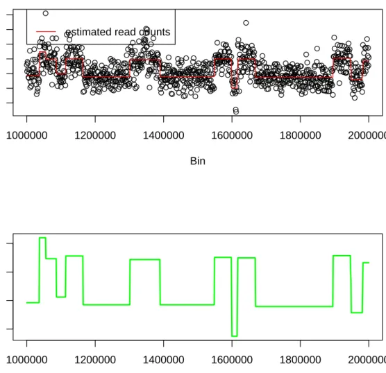
Figure 2.3: Read count data from human NGS of NA 19239 chromosome 6 with 1kb in each bin.-I  I  I  I
Figure 2.4: Display of read count data from NGS in a segment from bp position 6.0E+07 to 6.7E+07 in reference genome sequence
+7

References

Related documents

A sample of 108 women, aged between 35 and 55 years, completed questionnaire measures of body dissatisfaction, appearance investment, aging anxiety, media exposure (television

Prevalence and intensity of helminths found in stenodermatine bats from western Amazonian Brazil, and lick sites from which infected bats were captured.. Helminth Host Prevalence

The Government’s guidelines for external reporting for state- owned companies adopted in November 2007, (see pages 17–18 and 22–31) with special requirements on state-owned companies

The aim of our study was to analyze two sturgeon species, Huso huso and Acipenser ruthenus and their interspecific hybrid - bester, using nuclear markers, in order to set up

Learning and academic analytics in higher education is used to predict student success by examining how and what students learn and how success is supported by

Bankruptcy and Creditor Debtor Rights / Insolvency and Reorganization Law Litigation - Bankruptcy.

Beyond the implications outlined above (indications regarding managerial motives; insight into managerial challenges involved with mergers; identification of value-decreasing

Our consolidation solution is a disciplined, systematic approach that allows clients to realize significant operating cost savings in their enterprise contact centers..