1
OPTIMIZATION ISSUES IN WEB
SEARCH ENGINES
Zhen Liu
1and Philippe Nain
21IBM Research
Hawthorne, NY 10532, USA
[email protected] 2INRIA
B.P. 93, 06902, Sophia Antipolis Cedex, France
Abstract: Crawlers are deployed by a Web search engine for collecting information from different Web servers in order to maintain the currency of its data base of Web pages. We present studies on the optimization of Web search engines from different perspectives. We first investigate the number of crawlers to be used by a search engine so as to maximize the currency of the data base without putting an unnecessary load on the network. Both the static setting, where crawlers are always active, and the dynamic setting where, crawlers may be activated/deactivated as a function of the state of the system, are addressed. We then consider the optimal scheduling of the visits of these crawlers to the Web pages assuming these pages are modified at different rates. Finally, we briefly discuss some other optimization issues of Web search engines, including page ranking and system optimization.
Keywords: Web search engines, web crawlers, scheduling, optimal control, queues;
Markov decision process.
1.1 INTRODUCTION
The role of World Wide Web as a major information publishing and retrieving mech-anism on the Internet is now predominant and continues to grow extremely fast. The amount of information on the Web has long since become too large for manually browsing through any significant portion of its hypertext structure. As a consequence, a number of Web search engines have been developed in the last decade: starting from the pioneering search engines such as Alta Vista, Lycos, Infoseek, Magellan, Excite, to the most successful ones such as Yahoo and Google.
Search engines have become an indispensable utility for Internet users. According to a recent Pew Foundation Internet and Project (January 2005), “Search engines are highly popular among Internet users. Searching the Internet is one of the earliest activities people try when they first start using the Internet, and most users quickly feel comfortable with the act of searching. Users paint a very rosy picture of their online search experiences.”, and as of January 2005, “84% of internet users have used search engines. On any given day, 56% of those online use search engines.”
Thus, technologies that enhance Web search engines are of high practical interest. These search engines consist of indexing engines for constructing a data base of Web pages, and in many cases crawlers for bringing information to the indexing engine. To maintain currency and completeness of the data base, crawlers periodically make recursive traversals of the Web’s hypertext structure by accessing pages, then the pages referenced by these pages, and so on. In the literature one finds other colorful terms for crawler, such as wanderer, robot or spider, and the notion of a crawler being ‘routed to’ or ‘visiting’ a page. This chapter keeps with the ‘crawler’ and ‘accessing’ terminology throughout.
Traditionally, crawlers visit and index the Web pages until the data base reaches certain size. Periodically, this process is repeated through the rebuilding of a brand new data collection in replacement of the old one. Alternatively, the data base can be refreshed or updated incrementally. Such an operational mode is sometimes referred to as incremental crawler, see e.g. Cho and Garcia-Molina (2000b). Throughout this chapter, we consider the latter mode, i.e. the incremental crawler, although most anal-yses apply to the former as well.
Due to the critical role that these crawlers play in the Web search engines, the op-timization issues are topics of a number of research papers. In this chapter we present some of these research problems. Rather than providing comprehensive, but high-level, discussions, we present detailed solutions to some of the technical problems.
More precisely, Section 1.2 considers both the issues of optimizing the number of the crawlers to be deployed when all crawlers are always active (static setting – Section 1.2.1), and of finding an optimal decision rule for the case where crawlers may be activated/deactivated as a function of the state of the system (dynamic setting – Section 1.2.2). Performance of static and dynamic policies are compared in Section 1.2.3. The optimal scheduling of the page visits of these crawlers is studied in Section 1.3. Finally, we provide pointers to some other issues such as page ranking and system optimization (Section 1.4).
A word on the notation in use: bxc(respectivelydxe) denotes the largest (respec-tively smallest) integer less (respec(respec-tively greater) than or equal to x. Also for any mappings f and g, the relation f(x)∼xg(x)is understood as limx→∞f(x)/g(x) =1. 1.2 OPTIMIZING THE NUMBER OF CRAWLERS
We first address in Section 1.2.1 the situation where crawlers are always active, re-gardless of the state of the system, and we determine the optimal number of crawlers to be deployed. Then, we move in Section 1.2.2 to the situation where crawlers may be activated/deactivated as a function of the state of the system, and we find an optimal
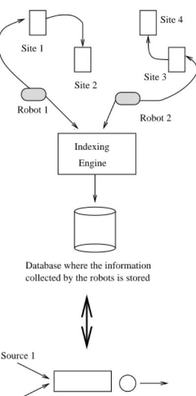
Engine Indexing Robot 1 Robot 2 Site 1 Site 2 Site 4 Site 3
Database where the information collected by the robots is stored
Source 1
Source 2 Server with a finite buffer
Figure 1.1 Model of search engine with two crawlers
decision rule for the number of active crawlers at any time. In both settings the cost function is a weighted sum of the starvation probability and loss rate.
The results presented in this section are based on the work of Talim et al. (2001b) and Talim et al. (2001a). Practical issues of deploying parallel crawlers are discussed in Cho and Garcia-Molina (2002).
1.2.1 The Static Setting
The search engine is modeled as a single server finite capacity queue. The system capacity is K≥2 (including the position in the server), see Figure 1.1.
There are N≥1 crawlers: each crawler brings new pages to the queue according to a Poisson process with rateλ>0. These N Poisson processes are assumed to be mutually independent and independent of the indexing (service) times. Hence, new pages are generated according to a Poisson process with intensityλN. An incoming
page finding a full queue is lost. Indexing times are assumed to be independent and identically random variables with common distribution F(x). Let 1/µ be the expected
The search engine is therefore modeled as the well known M/G/1/K queue (see e.g. Cohen (1982,Chapter III.6)). In this notation we define the cost function as the weighted sum of two terms:
the fraction of time that the system is empty, hereafter referred to as the
starva-tion probability;
the expected number of times when an arriving crawler finds a full system per unit time, hereafter referred to as the loss rate.
Let X (resp. X∗) be the stationary queue-length at arbitrary epochs (resp. stationary queue-length at arrival epochs) in a M/G/1/K queue with arrival rateλN and service
rate µ.
Withρ:=Nλ/µ>0 and forγ>0 the cost function is then defined as
C(ρ,γ,K):=γProb(X=0) +λN Prob(X∗=K) (1.1) with Prob(X=0)andλN Prob(X∗=K)the starvation probability and the loss rate, respectively. Since Prob(X∗=i) =Prob(X=i)for i=0,1, . . . ,K from the PASTA
property Wolff (1982), (1.1) rewrites as
C(ρ,γ,K) =γProb(X=0) +ρµ Prob(X=K) (1.2) whereλN in (1.1) has been replaced byρµ.
Throughout Section 1.2.1 we will assume that indexing times are exponentially distributed. The general case where the indexing times are arbitrarily distributed is more involved, due to the lack of closed-form expressions for the M/G/1/K queue, and is discussed in Talim et al. (2001b).
1.2.1.1 The M/M/1/K Search Engine Model. We assume that the
in-dexing times are exponentially distributed, namely, F(x) =1−exp(−µx). In other words, we model the search engine as an M/M/1/K queue.
In the M/M/1/K queue with traffic intensityρthe stationary queue-length probabil-ities at arbitrary epochs are given by Kleinrock (1975):
Prob(X=i) = 1−ρ 1−ρK+1ρ i (1.3) for i=0,1, . . . ,K. Therefore, C(ρ,γ,K) =(1−ρ)(γ+µρ K+1) 1−ρK+1 . (1.4) In particular, C(ρ,γ,K) = (γ+µ)/(K+1)whenρ=1.
Lemma 1 shows the existence of a unique minimum for C(ρ,γ,K)considered as a function ofρ. The proof is provided in Talim et al. (2001b).
Lemma 1 For anyγ>0, K≥2, the mappingρ→C(ρ,γ,K)has a unique minimum in[0,∞), to be denotedρ(γ,K). Furthermore, 0<ρ(γ,K)<1 ifγ<γ(K),ρ(γ,K) =1
We now return to the original problem, namely the computation of the number N of crawlers that minimizes the cost function C(ρ,γ,K)withρ=λN/µ. The answer is
found in the next result which is a direct corollary of Lemma 1.
Proposition 1 For anyγ>0, K≥2, let N(γ,K)be the optimal number of crawlers to use.
Then,
N(γ,K) =arg minnC(nλ/µ,γ,K) (1.5)
with n∈ {bρ(γ,K)µ/λc,dρ(γ,K)µ/λe}. Furthermore, N(γ,K)≤ dµ/λeifγ<γ(K), N(γ,K)∈ {bµ/λc,dµ/λe}ifγ=γ(K), and N(γ,K)≥ bµ/λcifγ>γ(K).
In the next section we investigate the impact of the parameterγ on the optimal number of crawlers.
1.2.1.2 Impact of γon the Optimal Number of Crawlers. Recall that
the parameterγis a positive constant that allows us to stress either the probability of starvation or the loss rate. Part of the impact ofγonρ(γ,K), and therefore on N(γ,K), the optimal number of crawlers, is captured in the following result.
Proposition 2 For any K≥2, the mappingγ→ρ(γ,K)is nondecreasing in(0,∞),
with limγ→∞ρ(γ,K) =∞.
Proof. Pick two constants 0<γ1<γ2and define
∆(ρ,γ1,γ2,K) := C(ρ,γ2,K)−C(ρ,γ1,K)
= 1−ρ
1−ρK+1(γ2−γ1).
We assume thatρ(γ2,K)<ρ(γ1,K)and show that this yields a contradiction.
Under the conditionγ1<γ2the mappingρ→∆(ρ,γ1,γ2,K)is decreasing in[0,∞).
Therefore,
0 < ∆(ρ(γ2,K),γ1,γ2,K)−∆(ρ(γ1,K),γ1,γ2,K)
= [C(ρ(γ2,K),γ2,K)−C(ρ(γ1,K),γ2,K)]
+ [C(ρ(γ1,K),γ1,K)−C(ρ(γ2,K),γ1,K)]
≤ 0, (1.6)
which contradicts the fact thatρ→∆(ρ,γ1,γ2,K)is decreasing in[0,∞). Therefore ρ(γ2,K)≥ρ(γ1,K)and the mappingγ→ρ(γ,K)is nondecreasing in[0,∞). We may
then define L :=limγ→∞ρ(γ,K).
From the identity∂C(ρ,γ,K)/∂ρ=0 forρ=ρ(γ,K)(see Lemma 1) we obtain 0 = µρ(γ,K)2(K+1)−(γK+µ(K+2))ρ(γ,K)K+1
0 1 2 3 4 5 6 7 8 0 1 2 3 4 5 6 K = 5 K=20
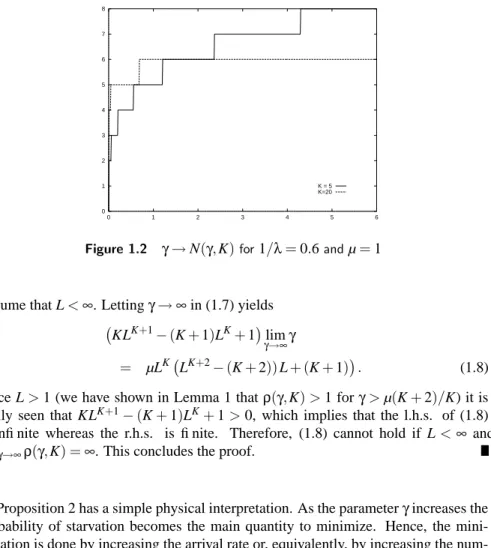
Figure 1.2 γ→N(γ,K)for1/λ=0.6andµ=1
Assume that L<∞. Lettingγ→∞in (1.7) yields
KLK+1−(K+1)LK+1
lim γ→∞γ
= µLK LK+2−(K+2))L+ (K+1)
. (1.8)
Since L>1 (we have shown in Lemma 1 thatρ(γ,K)>1 forγ>µ(K+2)/K) it is
easily seen that KLK+1−(K+1)LK+1>0, which implies that the l.h.s. of (1.8) is infinite whereas the r.h.s. is finite. Therefore, (1.8) cannot hold if L<∞ and limγ→∞ρ(γ,K) =∞. This concludes the proof.
Proposition 2 has a simple physical interpretation. As the parameterγincreases the probability of starvation becomes the main quantity to minimize. Hence, the mini-mization is done by increasing the arrival rate or, equivalently, by increasing the num-ber of crawlers, as shown in Proposition 2. Figure 1.2 provides two numerical exam-ples illustrating the monotonicity of the optimal number of crawlers as a function of
γ.
1.2.1.3 Impact of K on the Optimal Number of Crawlers. In this
section we examine the behavior ofρ(γ,K)as a function of K. The following results hold (see Talim et al. (2001b)):
Proposition 3
(a) If 0<γ≤µ then the mapping K→ρ(γ,K)is nondecreasing in[2,∞);
(b) Ifγ>µ then there exists an integer K0≥ b2u/(γ−λ)csuch that the mapping K→ρ(γ,K)is nondecreasing in[2,K0−1]and non-increasing in[K0,∞).
The next proposition examines the limiting behavior ofρ(γ,K)as K increases to in-finity.
Proposition 4 For anyγ>0,
lim
K→∞ρ(γ,K) =1. (1.9)
Proof. Let M :=limK→∞ρ(γ,K), where the existence of the limit follows from Proposition 3.
Letting now K→∞in (1.7) we see that the r.h.s. converges to−γif M<1 and converges to infinity if M>1, thereby showing that necessarily M=1, which con-cludes the proof.
Proposition 4 shows that the optimal arrival rate converges to the service capacity when the buffer size increases to infinity.
The limiting result (1.9) can be used to derive an approximation for the optimal number of crawlers to be deployed when K is large. Indeed, the relation
lim
K→∞N(γ,K) =Klim→∞argn∈{bµ/λminc,dµ/λe}C(λn/µ,γ,K), (1.10) which follows from (1.5), suggests the following approximation, for large K
N(γ,K)∼K dµ/λe if C(ρ+,γ,∞)≤C(ρ−,γ,∞) bµ/λc if C(ρ+,γ,∞)>C(ρ−,γ,∞) (1.11)
with the notation
C(ρ,γ,∞):=limK→∞C(ρ,γ,K),ρ+:= (λ/µ)dµ/λeandρ−:= (λ/µ)bµ/λc. Since C(ρ,γ,∞) =γ(1−ρ)forρ≤1 and C(ρ,γ,∞) =−µ(1−ρ)for ρ≥1 from (1.4), we may rewrite (1.11) as N(γ,K)∼K dµ/λe if−µ(1−ρ+)≤γ(1−ρ−) bµ/λc if−µ(1−ρ+)>γ(1−ρ−). (1.12)
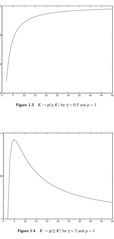
The mapping K→ρ(γ,K)is displayed in Figure 1.3 forγ<µ and in Figure 1.4
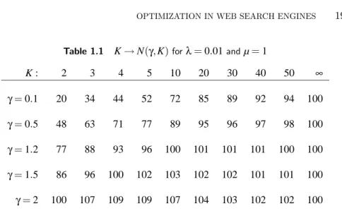
forγ>µ. Table 1.1 gives N(γ,K)for different values of K and compare these values with the approximation (1.12) (last column in Table 1.1). The approximation (1.12) appears to be fairly sensitive to model parameters; however, in all but one case (1.12) lies within 10% of the exact value as soon as K≥10. We also observe that the quality of the approximation increases whenγincreases (within 10% of the exact value for
0 5 10 15 20 25 30 35 40 45 50 0.4
0.6 0.8 1
Figure 1.3 K→ρ(γ,K)forγ=0.5andµ=1
0 5 10 15 20 25 30 35 40 45 50
1 1.05 1.1
Table 1.1 K→N(γ,K)forλ=0.01andµ=1 K : 2 3 4 5 10 20 30 40 50 ∞ γ=0.1 20 34 44 52 72 85 89 92 94 100 γ=0.5 48 63 71 77 89 95 96 97 98 100 γ=1.2 77 88 93 96 100 101 101 101 100 100 γ=1.5 86 96 100 102 103 102 102 101 101 100 γ=2 100 107 109 109 107 104 103 102 102 100
1.2.2 The Dynamic Setting
In this section we assume that the number of active crawlers may vary in time ac-cording to the backlog in the queue and to the number of crawlers already active. To address this situation we will cast our model into the Markov Decision Process (MDP) framework (Bertsekas, 1987; Puterman, 1994; Ross, 1983).
The indexing engine is again modeled as a finite-capacity single-server queue. Ser-vice times still constitute independent random variables with common negative expo-nential distribution (with mean 1/µ) and the buffer may accommodate at most K≥2 customers, including the one in service, if any. There are N available crawlers and each of these crawlers, when activated, brings pages to the server according to a Pois-son process with rate λ. We assume that these N Poisson processes are mutually independent and further independent of the service time process.
The new feature in this section is that the number of active crawlers may be mod-ified at any arrival and at any departure epoch. When an arrival occurs, the incoming crawler is deactivated at once; the controller may then decide to keep it idle or to re-activate it. When a departure occurs the controller may either decide to re-activate one additional crawler, if any available, or to do nothing (i.e. the number of active crawlers is not modified).
The objective is to find a policy (to be defined) that minimizes a weighted sum of the stationary starvation probability and the loss rate.
We now introduce the MDP setting in which we will solve this optimization problem. Since the time between transitions is variable we will use the uniformization method (Bertsekas, 1987,Sec. 6.7).
At the n-th decision epoch tnthe state of the MDP is represented by the triple xn= (qn,rn,sn)∈ {0,1, . . . ,K} × {0,1, . . . ,N} × {0,1,2}, with qnand rnthe queue-length and the number of active crawlers just before the n-th decision epoch, respectively, and snthe type (arrival, departure, fictitious – see below) of the n-th decision epoch.
The successive decision epochs{tn,n≥1}are the jump times of a Poisson process with intensityν:=λN+µ, independent of the service time process. In this setting, the n-th decision epoch tncorresponds to an arrival in the original system with probability
λrn/ν(in which case sn=1), to a departure with probability µ/νprovided that qn>0 (sn=0) and to a fictitious event with the complementary probability((N−rn)λ+µ)/ν (sn=2).
Let an∈ {0,1}be the action chosen at time tn. We assume that an=1 if the decision is made to activate one additional crawler, if any available, and an=0 if the decision is made to keep unchanged the number of active crawlers. By convention we assume that an=0 if the n-th decision epoch corresponds to a fictitious event (sn=2).
From the above definitions we see that states of the form(•,0,1)and(0,•,0)are not feasible, as an arrival cannot occur if all crawlers are inactive and a departure cannot occur if the queue is empty, respectively. Therefore, the state-space for this MDP is
{(q,r,s),0≤q≤K,0≤r≤N,s=0,1,2}
−{(0,r,0),(q,0,1),0≤q≤K,0≤r≤N}.
However, this set contains one absorbing state, the “fictitious” state(0,0,2). To re-move this undesirable state we will only consider policies (see formal definition be-low) that always choose action a=1 when the system is in state(1,0,0)so that(0,0,2) can never be reached. This is not a severe restriction since a policy that never activates crawlers when the system is empty is of no interest. In conclusion, the state space for this MDP is
X :={(q,r,s),0≤q≤K,0≤r≤N,s=0,1,2}
−{(0,0,2),(0,r,0),(q,0,1),0≤q≤K,0≤r≤N}
and the set Axof allowed actions when the system is in state x= (q,r,s)∈X is given by Ax= {0} if s=2 {1} if(q,r,s) = (1,0,0) {0,1} otherwise.
To complete the definition of the MDP we need to introduce the one-step cost c and the one-step transition probabilities p. Given that the process is in state x= (q,r,s) and that action a is made, the one-step cost is defined as
c(x) =γ1(q=0) +ν1(q=K,s=1), (1.13) independent of a. We will show later on in this section that this choice for the one-step cost will allow us to address, and subsequently to solve, the optimization problem at hand.
For x∈X, the one-step transition probabilities px,x0(a)are given by px,x0(a) = µ ν1(q>1) if x0= (q−1,min{r+a,N},0) λr ν if x0= (q−1,min{r+a,N},1) 1−µ 1(q>1)−λr ν if x0= (q−1,min{r+a,N},2) (1.14) if s=0, a=0,1; px,x0(a) = µ ν if x0= (min{q+1,K},r+a−1,0) λ(r+a−1) ν if x0= (min{q+1,K},r+a−1,1) 1−µ+λ(r+a−1) ν if x0= (min{q+1,N},r+a−1,2) (1.15) if s=1, a=0,1; px,x0(0) = µ ν1(q>0) if x0= (q,r,0) λr ν if x0= (q,r,1) 1−µ 1(q>0) +λr ν if x0= (q,r,2) (1.16)
if s=2. All other transition probabilities are equal to 0.
Without loss of generality we will only consider pure stationary policies since it is known that nothing can be gained by considering more general policies (Puterman, 1994,Ch. 8-9). Recall that in the MDP setting a policyπis pure stationary if, at any decision epoch, the action chosen is a non-randomized and time-homogeneous map-ping of the current state (Bertsekas, 1987; Puterman, 1994; Ross, 1983). We define an
admissible stationary policy as any mappingπ: X→ {0,1}such thatπ(x)∈Ax. For later use introduce P(π):= [px,x0(π(x))](x,x0)∈X×X, the transition probability
ma-trix under the stationary policyπ.
Let
P
be the class of all admissible stationary policies. For any policy π∈P
introduce the long-run expected average cost per unit timeWπ(x) =lim n→∞ 1 nEπ " n
∑
i=1 c(xi)|x1=x # , x∈X. (1.17) The existence of the limit in (1.17) is a consequence of the fact thatπis stationary and X is countable (Puterman, 1994,Proposition 8.1.1).We shall say that a policyπ?∈
P
is average cost optimal ifWπ?(x) = inf
π∈PWπ(x) ∀x∈X. (1.18) In order to use results from MDP theory for average cost models we first need to determine to which class (recurrent, unichain, multichain, communicating, etc.) the current MDP belongs to. Consider the following example: N=2 and let πbe any stationary policy that selects action 1 in states(•,r,1)for r∈ {1,2}and in state (1,0,0), and action 0 otherwise. It is easily seen that this policy induces a MDP with two recurrent classes (X∩ {(•,1,•)}and X∩ {(•,2,•)} and a set of transient states (X∩ {•,0,•}). We therefore conclude from this example that the MDP{xn,n≥1}is
multichain (Puterman, 1994,p. 348).
An MDP is communicating (Puterman, 1994,p.348) if, for every pair of states (x,x0)∈X×X, there exists a stationary policy π such that x0 is accessible from x, that is, if there exists n≥1 such that Px,xn 0(π)>0, where Px,xn 0(π)is the(x,x0)-entry of
the matrix Pn(π).
Lemma 2 The MDP(xn,n≥1)is communicating. The proof of Lemma 2 is given in (Talim et al., 2001a). The next result follows from Lemma 2 and Proposition 4 in (Bertsekas, 1987,Sec. 7.1):
Proposition 5 There exists a scalarθand a mapping h : X→IR such that, for all x∈X,
θ+h(x) =c(x) +min a∈Axx
∑
0∈Xpx,x0(a)h(x0) (1.19)
withθ=infπ∈PWπ(x)for all x∈X, while ifπ?(x)attains the minimum in (1.19) for
each x∈X, then the stationary policyπ?is optimal.
The optimal average costθand the optimal policyπ?in Proposition 1.17 can be computed by using the following recursive scheme, known as the relative value itera-tion algorithm.
Proposition 6 Let ˆx be a fixed state in X and 0<τ<1 be a fixed number. For k≥0,
x∈X, define the mappings(hk,k≥0)as
hk+1(x) = (1−τ)hk(x) +τ(T(hk)(x)−T(hk)(ˆx)) with
T(hk)(x):=c(x) +min a∈Axx
∑
0∈Xpx,x0(a)hk(x0),
where h0(xˆ) =0 but otherwise h0is arbitrary.
Then, the limit h(x) =limk→∞hk(x)exists for each x∈X,θ=τT(h)(xˆ), and the
optimal actionπ?(x)in state x is given byπ?(x)∈argmina∈A
x∑x0∈Xpx,x0(a)h(x0). Proof. Since the MDP is communicating (cf. Lemma 2) the proof follows from Puterman (1994,Sec. 8.5,9.5.3) (see also Bertsekas (1987,Prop. 4, p. 313 )).
We now return to our initial objective, namely, minimizing a weighted sum of the stationary starvation probability and the loss rate. To see why the solution to this problem is given by the solution to the MDP problem formulated in this section, it suffices to show that the average cost (1.17) is a weighted sum of the stationary star-vation probability and the loss rate. It should be clear, however, that this result cannot hold for policies that induce an average cost (1.17) that depends on the initial state x as, by definition, the stationary starvation probability and the loss rate are independent of the initial state. We will therefore restrict ourselves to the class
P
0⊂P
of policiesthat generate a constant average cost, namely,
P
0={π∈P
: Wπ(x) =Wπ(x0),∀x∈X}.The set
P
0 is non-empty as it is well-known that it contains, among others, allunichain policies (Puterman, 1994,Proposition 8.2.1). Among such policies is the
static policyπN that always maintain N crawlers active, namely,πN(x) =1 for all
x= (•,•,s)∈X with s=0,1 andπN(x) =0 for all x= (•,•,2)∈X.
We may also note that reducing the search for an optimal policy to policies in
P
0does not yield any loss of generality as it is also known that there always exitsan optimal policy with constant average cost in the case of communicating MDP’s (Puterman, 1994,Proposition 8.3.2).
Fixπ∈
P
0. Introducing (1.13) into (1.17) yields Wπ(x) =γSπ(x) +Lπ(x)withSπ(x) = lim n→∞ 1 nEπ "n
∑
i=1 1(qi=0)|x1=x # Lπ(x) = νlim n→∞ 1 nEπ " n∑
i=1 1(qi=K,si=1)|x1=x # .In the following we will drop the argument x in Sπ(x)and Lπ(x)since these quantities do not depend on x from the definition of
P
0.Let us now interpret Sπ and Lπ. Sπ is the stationary probability that the system is empty at decision epochs. Since the decision epochs form a Poisson process, we may conclude from the PASTA property (Wolff, 1982) that Sπ is also equal to the stationary probability that the system is empty at arbitrary epoch with is nothing but the stationary starvation probability.
Let us now consider Lπ. Recall that{tn,n≥1}, the successive decision instants, is a Poisson process with intensityνand assume without loss of generality that t1=0 a.s.
Define A(t)as the total number of customers that have arrived to the queue up to time
t, including customers which have been lost, and let Q(t)be the queue length at time
t. We assume that the sample paths of the processes{A(t),t≥0}and{Q(t),t≥0} are right-continuous with left limit. With these definitions and the identity E[tn] =n/ν
we may rewrite Lπas Lπ=lim n→∞ EπR0tn1(Q(t−) =K)dA(t) E[tn] .
In other words, we have shown that Lπis the ratio, as n tends to infinity, of the expected number of losses during the first n decision epochs over the expected occurrence time of the n-th decision epoch.
The interpretation of Lπas a loss rate now follows from the identity Lπ = lim n→∞ EπRtn 0 1(Q(t−) =K)dA(t) E[tn] = lim T→∞ 1 T Eπ Z T 0 1( Q(t−) =K)dA(t) , ∀π∈
P
0, (1.20)upon noticing that the latter quantity represents the mean number of losses per unit time or the loss rate. The second identity in (1.20) is a direct consequence of the theory of renewal reward processes (Ross, 1983,Theorem 7.5) and of the definition of the set
P
0.In summary, we have shown that for any policyπin
P
0the average cost is Wπ=γSπ+Lπ,with Sπthe starvation probability and Lπthe loss rate.
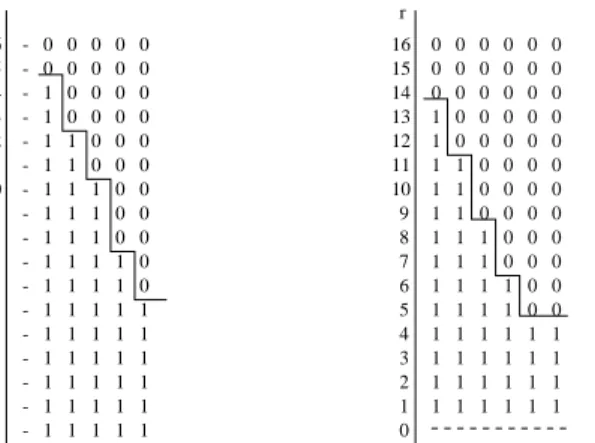
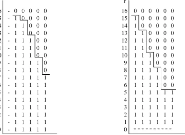
The optimal policy has been computed for different values of the model parame-ters. Figures 1.5-1.7 display the optimal policy for N=16, K=5,λ=0.1, µ=1 and for different values ofγ(γ<γ(K) =1.4, γ=γ(K)andγ>γ(K)). The results were obtained by running the value iteration algorithm given in Proposition 6 with the stopping criterion maxx∈X|(hk+1(x)−hk(x))/hk(x)|<10−5(254, 255 and 256
iter-ations were needed to compute the optimal policy displayed in Figures 1.5, 1.6 and 1.7, respectively). We see from these figures that the optimal policy is a monotone
switching curve, namely, there exist two monotone (decreasing here) integer
map-pings fs :{0,1, . . . ,N} → {0,1,2, . . .}, s∈ {0,1}, such thatπ?(x) =1(fs(r)≥q)for all x= (q,r,s)∈X with s=0,1 (we must also have f0(0)≥1 so thatπ?(1,0,0) =1 as
required). We conjecture that the optimal policy always exhibits such a structure but we have not able been to prove it.
s = 0 s = 1 16 15 14 13 12 11 10 9 8 7 6 5 4 3 2 1 0 r - 1 1 1 1 1 - 1 1 1 1 1 - 1 1 1 1 1 - 1 1 1 1 1 - 1 1 1 1 1 - 1 1 1 1 1 - 1 1 1 1 0 - 1 1 1 1 0 - 1 1 1 0 0 - 1 1 1 0 0 - 1 1 1 0 0 - 1 1 0 0 0 - 1 1 0 0 0 - 1 0 0 0 0 - 1 0 0 0 0 - 0 0 0 0 0 - 0 0 0 0 0 0 1 2 3 4 5 q 16 15 14 13 12 11 10 9 8 7 6 5 4 3 2 1 0 r 0 1 2 3 4 5 q 1 1 1 1 1 1 1 1 1 1 1 1 1 1 1 1 1 1 1 1 1 1 1 1 1 1 1 1 0 0 1 1 1 1 0 0 1 1 1 0 0 0 1 1 1 0 0 0 1 1 0 0 0 0 1 1 0 0 0 0 1 1 0 0 0 0 1 0 0 0 0 0 1 0 0 0 0 0 0 0 0 0 0 0 0 0 0 0 0 0 0 0 0 0 0 0
Figure 1.5 Optimal policy (γ=1, Cost = 0.20907)
s = 0 s = 1 - 1 1 1 1 1 - 1 1 1 1 1 - 1 1 1 1 1 - 1 1 1 1 1 - 1 1 1 1 1 - 1 1 1 1 1 - 1 1 1 1 1 - 1 1 1 1 0 - 1 1 1 1 0 - 1 1 1 0 0 - 1 1 1 0 0 - 1 1 1 0 0 - 1 1 0 0 0 - 1 1 0 0 0 - 1 0 0 0 0 - 1 0 0 0 0 - 0 0 0 0 0 16 15 14 13 12 11 10 9 8 7 6 5 4 3 2 1 0 r 16 15 14 13 12 11 10 9 8 7 6 5 4 3 2 1 0 r 0 1 2 3 4 5 q 0 1 2 3 4 5 q 1 1 1 1 1 1 1 1 1 1 1 1 1 1 1 1 1 1 1 1 1 1 1 1 1 1 1 1 0 0 1 1 1 1 0 0 1 1 1 1 0 0 1 1 1 0 0 0 1 1 1 0 0 0 1 1 0 0 0 0 1 1 0 0 0 0 1 1 0 0 0 0 1 0 0 0 0 0 1 0 0 0 0 0 0 0 0 0 0 0 0 0 0 0 0 0
s = 0 s = 1 16 15 14 13 12 11 10 9 8 7 6 5 4 3 2 1 0 r 16 15 14 13 12 11 10 9 8 7 6 5 4 3 2 1 0 r 0 1 2 3 4 5 q - 1 1 1 1 1 - 1 1 1 1 1 - 1 1 1 1 1 - 1 1 1 1 1 - 1 1 1 1 1 - 1 1 1 1 1 - 1 1 1 1 1 - 1 1 1 1 1 - 1 1 1 1 0 - 1 1 1 1 0 - 1 1 1 0 0 - 1 1 1 0 0 - 1 1 1 0 0 - 1 1 0 0 0 - 1 1 0 0 0 - 1 0 0 0 0 - 0 0 0 0 0 0 1 2 3 4 5 q 1 1 1 1 1 1 1 1 1 1 1 1 1 1 1 1 1 1 1 1 1 1 1 1 1 1 1 1 1 1 1 1 1 1 0 0 1 1 1 1 0 0 1 1 1 1 0 0 1 1 1 0 0 0 1 1 1 0 0 0 1 1 0 0 0 0 1 1 0 0 0 0 1 1 0 0 0 0 1 0 0 0 0 0 1 0 0 0 0 0 0 0 0 0 0 0
Figure 1.7 Optimal policy (γ=2, Cost = 0.32211)
1.2.3 Static Versus Dynamic Policies
In this section we compare static and dynamic policies in the case where the indexing times are exponentially distributed. The results are reported in Tables 1.2 and 1.3. Throughout the experiments µ=1. For different sets of parametersλ,K,γ, we first computed the optimal number of crawlers Ns(given by Proposition 1) and the average cost Cs(given in (1.4)) in the static setting.
Then, for each set of parametersλ,K,γ, we set the value of the number of available crawlers N to Ns and determined, via the relative value iteration algorithm given in Proposition 6 (withτ=0.99999 – the closerτis from 1 the faster the algorithm con-verges), the optimal average cost Cd(given in (1.18)) as well as the minimum (Nmin)
and the expected (N) number of crawlers activated by the optimal dynamic policy. These results can be found in Table 1.2.
We stopped the numerical procedure when the relative error between two consec-utive iterates was (uniformly) less than 10−5. The number of iterations (Niter) and the
relative improvement (100%×(Cs−Cd)/Cd) are also reported in Table 1.2.
Last, we computed the overall optimal dynamic policy by removing the restriction on the number of available crawlers. The optimal average cost Cd as well as the minimum (Nmin), expected (N) and maximum (Nmax) number crawlers used by the
overall optimal dynamic policy are given in Table 1.3.
We observe that substantial gains may be achieved by dynamically controlling the activity of the crawlers. When the number of available crawlers is set to Ns(Table 1.2) the relative improvement w.r.t. to the optimal static policy ranges from 4% to 103% for the considered model parameters; when the restriction on the number of avail-able crawlers is removed then the improvement ranges from 6% to 3226%! The gain appears to be an increasing function of the queue size K and of the arrival rateλ.
Table 1.2 Static vs. dynamic policies (withµ=1andτ=0.99999)
Static Approach Dynamic Approach
λ K γ Cs Ns Cd Nmin N¯ Niter Rel. Impr.
0.01 5 0.4 0.17541 73 0.16804 57 70.3 1634 4% - - 1.4 0.40000 100 0.38336 86 95.1 1911 4% - - 2.4 0.53834 114 0.51746 101 108.4 2051 4% 0.01 10 0.4 0.10207 86 0.09062 60 82.6 1794 13% - - 1.2 0.20000 100 0.17534 77 94.1 1939 14% - - 2.4 0.28347 110 0.24798 88 102.3 2039 14% 0.01 15 0.4 0.07177 91 0.05891 58 87.7 1860 22% - - 1.13 0.13313 100 0.10720 70 94.5 1953 24% - - 2.4 0.19192 107 0.15342 78 99.7 2024 25% 0.05 5 0.4 0.17578 15 0.15127 7 13.8 338 16% - - 1.4 0.40000 20 0.34733 12 17.7 391 15% - - 2.4 0.53841 23 0.46583 15 20.2 422 16% 0.05 10 0.4 0.10220 17 0.08308 5 16.2 369 23% - - 1.2 0.20000 20 0.14955 8 18.2 402 34% - - 2.4 0.28347 22 0.20541 10 19.4 423 38% 0.05 15 0.4 0.07184 18 0.05514 4 17.4 401 30% - - 1.13 0.13313 20 0.09117 6 18.7 426 46% - - 2.4 0.19372 21 0.13895 8 19.3 438 39% 0.1 5 0.4 0.17600 7 0.15239 1 6.5 167 15% - - 1.4 0.40000 10 0.32198 4 8.6 200 24% - - 2.4 0.54067 11 0.44989 5 9.3 211 20% 0.1 10 0.4 0.10403 9 0.06838 0 8.4 204 52% - - 1.2 0.20000 10 0.13854 2 9.0 218 44% - - 2.4 0.28347 11 0.18585 3 9.6 227 53% 0.1 15 0.4 0.07184 9 0.05326 0 8.7 312 35% - - 1.13 0.13313 10 0.08538 1 9.3 359 56% - - 2.4 0.19458 11 0.09606 1 9.7 376 103%
Table 1.3 Static vs. dynamic policies (withµ=1andτ=0.99999)
Static Approach Dynamic Approach
λ K γ Cs Ns Cd Nmin N¯ Nmax Rel. Impr.
0.01 5 0.4 0.17541 73 0.16595 58 74.8 82 6% - - 1.4 0.40000 100 0.37886 88 99.9 115 6% - - 2.4 0.53834 114 0.51179 103 113.0 133 5% 0.01 10 0.4 0.10207 86 0.08124 62 89.3 105 27% - - 1.2 0.20000 100 0.15876 78 99.6 123 26% - - 2.4 0.28347 110 0.22777 89 107.1 137 24% 0.01 15 0.4 0.07177 91 0.04236 59 94.9 118 69% - - 1.13 0.13313 100 0.07812 71 99.8 131 70% - - 2.4 0.19192 107 0.11493 79 103.6 143 67% 0.05 5 0.4 0.17578 15 0.13770 7 15.9 20 28% - - 1.4 0.40000 20 0.31712 13 19.8 27 26% - - 2.4 0.53841 23 0.43292 16 21.9 32 24% 0.05 10 0.4 0.10220 17 0.04128 5 19.0 29 148% - - 1.2 0.20000 20 0.12020 8 19.9 33 66% - - 2.4 0.28347 22 0.20541 10 20.6 36 38% 0.05 15 0.4 0.07184 18 0.00969 2 19.8 35 641% - - 1.13 0.13313 20 0.01818 4 20.0 38 632% - - 2.4 0.19372 21 0.02782 6 20.1 41 596% 0.1 5 0.4 0.17600 7 0.11097 2 8.2 12 59% - - 1.4 0.40000 10 0.25924 4 9.8 16 54% - - 2.4 0.54067 11 0.35805 6 10.7 18 51% 0.1 10 0.4 0.10403 9 0.01937 0 9.7 18 437% - - 1.2 0.20000 10 0.03887 1 9.9 20 415% - - 2.4 0.28347 11 0.05894 2 10.1 22 381% 0.1 15 0.4 0.07184 9 0.00188 0 10.0 24 3721% - - 1.13 0.13313 10 0.00368 0 10.0 25 3518% - - 2.4 0.19458 11 0.00585 0 10.0 27 3226%
1.3 OPTIMAL SCHEDULING OF THE CRAWLERS
We now turn to the problems of scheduling a crawler that maintains the currency of existing pages in search-engine data bases. For sake of arguments, we assume that the set of Web pages is fixed. However, as we shall see, our results can be promoted as
heuristics that acquire new pages and drop old pages over time. A specific objective will be to find crawler schedules that minimize the obsolescence of the data base in some useful sense. For example, assume there are N Web pages, labeled 1,2, . . . ,N,
which are to be accessed repeatedly by a crawler, the duration of each access being an independent sample from a given distribution. Assume also that the contents of page i are modified at times that follow a Poisson process with parameter µi. A page is considered up-to-date by the indexing engine from the time it is accessed by the crawler until the next time it is modified, at which point it becomes out-of-date until the crawler’s next access. Let ri be the fraction of time page i spends out-of-date. The problem is to find relative page-access frequencies and a sequencing policy that realizes these frequencies such that the objective function C=∑1≤i≤Nciri, is mini-mized, where the ciare given weights. Under simplifying but plausible assumptions on the weights, page access times, and the class of allowed policies, we obtain explicit solutions to this problem.
From a theoretical point of view, our problem is closely related to those multiple-queue single-server systems usually called polling systems in the multiple-queueing literature. Indeed, the crawler can be considered as the server and the pages as the stations in the polling system. The durations of consecutive page accesses correspond to switch-over times and the page modifications correspond to customer arrivals. The service times in this polling system are zero. Our two-stage approach of optimizing crawler schedules (determining access frequencies and then finding a schedule that realizes them) is similar to the approach in Borst (1994), Borst et al. (1994) and Boxma et al. (1993) of optimizing visit sequences in polling systems.
An extensive literature exists on the analysis and control of polling systems. The interested reader is referred to the book of Takagi (1986) for general references; the special issue of the journal Queueing Systems, Vol. 11 (1992) on polling models and the recent thesis of Borst (1994) can be consulted for more recent developments. In particular, the polling systems with zero service times were motivated by communi-cation networks such as teletext and videotex where pages of information are to be broadcast to terminals connected to a computer network (Ammar and Wong, 1987; Dykeman et al., 1986; Liu and Nain, 1992). However, the problem here has not been analyzed. Indeed, in the usual analysis of polling systems with unbounded buffers, in-terest centers on mean waiting times and mean queue lengths, whereas in our problem, the performance measure of interest, viz., the obsolescence time, corresponds to the maximum waiting time of a customer during a visit cycle of the server. An alternative view of our model identifies it with a polling loss system having unit buffers, in which our obsolescence time becomes the waiting time. With this point of view, our model has potential use in maintenance applications.
The next subsection is devoted to a precise formulation of our model, and a review of some useful concepts in stochastic ordering theory. Section 1.3.2 begins by prov-ing two properties of crawler schedulprov-ing policies: (i) expected obsolescence times increase as the page-access time increases in the increasing-convex-ordering sense, and (ii), by Schur-convexity results, accesses to any given page should be as evenly spaced as possible. We then derive a tight lower bound on the cost function C assum-ing that the weights ci are proportional to the µi. These results yield a formula for
optimal access frequencies. Our techniques can be extended to general ci, but explicit formulas are not attainable in general.
To motivate the assumption on weights, note that a useful choice for the ci is the customer page-access frequency, for in this case the total cost can be regarded as a customer total error rate. The special case where the customer access frequency ci is proportional to the page-change rate µ is reasonable under this interpretation - the greater the interest (access frequency), the greater the frequency of page modification.
Sections 1.3.3 and 1.3.4 deal with the problem of sequencing page accesses opti-mally, or near optiopti-mally, so as to realize a given set of access frequencies. This mate-rial is prefaced by a discussion at the end of Section 1.3.2 which relates our scheduling problem to those that come under the heading of generalized round-robin or template-driven scheduling.
In Section 1.3.3, we introduce randomized page accessing, where each access is determined by an independent and identically distributed (i.i.d.) sample from a distri-bution{fi}. We show how to find that choice for this distribution which minimizes C. In Section 1.3.4, we develop a policy that performs well when N is large. It is based on work of Itai and Rosberg (1984) (in an entirely different setting) and yields a cost within 5% of optimal.
Results presented in this section are based on the work of Coffman Jr. et al. (1998). A related study was conducted in Cho and Garcia-Molina (2000a).
1.3.1 Preliminaries
Let{Xk}be the sequence of durations of consecutive page accesses by the crawler, each Xkbeing distributed independently as a random variable X . For scheduling policy
π, letπn∈ {1,2, . . . ,N}be the scheduling decision for the n-th access, i.e., the index of the n-th page to be accessed by the crawler underπ. Define the inter-access distance
dij(π) =nij(π)−nij−1(π), where ni
j(π)is the index of the j-th access of page i, i.e.,
nij(π) =inf{n>nij−1(π)|πn=i}, and where ni0(π)≡0. Let Xij=Xij(π)be the j-th inter-access time of page i, i.e., j-the time between j-the (j−1)-st and j-th page-i access completion times. We have Xij=∑n
i j
k=nij−1+1Xk, so the random variables X
i jare mutually independent. Note that, if page access times Xkare exponentially distributed, then Xi
jhas an Erlang distribution of dijstages.
Hereafter, except in definitions, the policyπ will normally be omitted from our notation; in such cases, the policy will always be clear in context.
Let Zij =Zij(π)be the time that page i is out-of-date during the j-th inter-access time of page i. Let min=min(π)be the number of accesses of page i among the first
n accesses: min=∑nk=1
1
{πk=i}, where1
{·}is the indicator function. Hereafter, we consider only stationary scheduling policies in the sense that, for each such policy, the limitfi=fi(π) = lim n→∞
min
n (1.21)
exists and is strictly positive for all i, 1≤i≤N. We call fithe access frequency of page i. We also require that the limits limn→∞∑nj=1Zij/n and limn→∞∑nj=1E[Zij]/n
exist and be equal. These last assumptions hold under fairly mild conditions, e.g., when the sequence{di
j(π)}jis stationary and ergodic (cf. Kingman (1968)).
The obsolescence rate ri=ri(π)of page i is the limiting fraction of time that page
i is out of date; precisely, it is defined as
ri=lim n→∞ ∑min j=1Zij ∑mi n j=1Xij = lim n→∞ ∑min j=1Zij n lim n→∞ ∑min j=1Xij n = 1 E[X]·nlim→∞ ∑min j=1E[Zij] n . (1.22)
In particular, when policyπis cyclic with cycle length K, i.e., whenπnK+k=π(n−1)K+k for all 1≤k≤K and all n=1,2, . . ., then
ri= 1 KE[X] miK
∑
j=1 E[Zij], (1.23)where miK is the number of page-i accesses during a cycle. The cost function to be minimized is the weighted sum of the obsolescence rates:
C=C(π) = N
∑
i=1ciri, (1.24) where ciare given positive real numbers and the minimization is to be over all station-ary scheduling policies.
A few basics in stochastic ordering conclude this section. For two m-dimensional real vectors x and y, x majorizes y, written xy, if ∑ki=1x[i]≥∑ki=1y[i], for k= 1, . . . ,m−1 and∑mi=1x[i]=∑m
i=1y[i], where x[i] is the ith largest component of x.
In-tuitively, y is better balanced than x. A function h is said to be Schur-convex if
h(x)≥h(y)whenever xy. See Marshall and Olkin (1979) for more details about this and related properties.
A random variable Y1is said to be no greater than a random variable Y2in the convex
ordering sense, denoted Y1≤cxY2, if E[h(Y1)]≤E[h(Y2)]for all convex functions h,
provided the expectations exist. If in this definition ‘convex’ is replaced everywhere by ‘increasing and convex,’ then we write Y1≤icxY2. As is easily verified, Y1≤cxY2
implies that Y1has the same mean but smaller variance than Y2. It is also easy to see
that Y1≤cxY2 implies Y1≤icxY2. See Stoyan (1933) for equivalent definitions and
further properties.
1.3.2 Schur Convexity and a Lower Bound
Recall that a page is considered out-of-date from the time it is modified until the next time it is accessed by the crawler. Thus, if page i is not modified during its j-th inter-access interval, then the obsolescence time is Zi
j=0. Otherwise, Zij is the time that elapses from the first moment page i is modified during its j-th inter-access interval until the end of that interval. Recall also that the modification (or mutation) epochs of page i follow a Poisson process with parameter µi. By the memoryless property of the
Poisson process, the time that elapses from the beginning of page i’s j-th inter-access interval to the first subsequent mutation has an exponential distribution with parameter
µi. Let Ri1,Ri2, . . .be an i.i.d. sequence of such random variables, so that
Zij=d Xij−Rij+, (1.25) where x+denotes max(x,0)and=d denotes equality in distribution.
As an immediate consequence, we obtain
Proposition 7 If the page access time is decreased in the increasing convex ordering
sense, then the obsolescence rate is decreased for all pages under any scheduling policy.
Proof. Let{Xk0}be a sequence of access times distributed independently as X0, and define{X0ij}jand{Z0ij}jas for Xk. Assume that X0≤icxX . Then,
Z0ij=d X0ij−Rij+≤icx Xji−Rij + d =Zij, and so E[Z0ij]≤E[Zij]. Thus, ri0= 1 E[X0]·nlim→∞ ∑min j=1E[Z0 i j] n ≤ 1 E[X]·nlim→∞ ∑min j=1E[Zij] n =ri, as desired.
Returning to our main problem, where the distribution of page access times is as-sumed given, we now show that the obsolescence rate is a Schur convex function of the vector of inter-access distances. For this, we need the following calculation which will also be useful for later results. Define hi=E[e−µiX], the Laplace transform of X evaluated at µi.
Lemma 3 For any page i,
E[Zij] =dijE[X]−µ1 i 1−hd i j i .
Proof. Let Gijbe the probability distribution of Xij. We have from (1.25) that
E[Zij] = Z ∞ 0 P(Zij>z)dz = Z ∞ 0 P(Xij−Rij>z)dz = Z ∞ 0 Z ∞ z 1−e−µi(x−z)·Gi j(dx)dz = Z ∞ 0 Z x 0 1−e−µi(x−z)dzGi j(dx) = Z ∞ 0 x−1−e −µix µi Gij(dx)
which yields the lemma.
We can conclude from the above proof that the result of Proposition 7 still holds when the increasing convex ordering is replaced by the weaker Laplace-transform ordering (see Stoyan (1933)). It follows from a result of Schur (cf. Marshall and Olkin (1979,Proposition 3.C.1, page 64)) and Lemma 3 that
Proposition 8 For any fixed number n of page-i accesses, the expected total
obso-lescence time of page i, ∑ni=1E[Zij]is a Schur convex function of the distances dij, j=1, . . . ,n.
Thus, in order to minimize the expected obsolescence time, the accesses to any particular page should be as evenly spaced as possible.
An algorithm that computes a schedule of the crawler that implements a given set of access frequencies in the sense of (1.21) is called an accessing policy. In these terms, the scheduling policies proposed in this paper consist of two stages; the first computes a set of access frequencies{fi}and the second is an accessing policy that implements{fi}. The even-spacing objective of accessing policies yields a lower bound, as follows.
Proposition 9 The obsolescence rate under any accessing policy implementing the
access frequencies{fi}satisfies for each i,
ri≥ 1 E[X] E[X]−µfi i + fi µi h1/fi i . Proof. ri = 1 E[X]·nlim→∞ ∑mi n j=1E[Zij] n = 1 E[X]·nlim→∞ 1 n mi n
∑
j=1 dijE[X]− 1 µi 1−hd i j i = 1 E[X]·nlim→∞ 1 n nE[X]−m i n µi + 1 µi mi n∑
j=1 hd i j i = 1 E[X] E[X]−µfi i +1 µi lim n→∞ 1 n min∑
j=1 hd i j i ≥ E[1X] E[X]−µfi i + 1 µi lim n→∞ min n h n/mi n i = 1 E[X] E[X]− fi µi + fi µi h1/fi i ,where the inequality comes from the Schur convexity of ∑min j=1h
di j
i in the dij’s (cf. Proposition 8).
The above lower bound can be achieved only in special cases. For instance, if the frequencies are all equal, the policy that accesses pages 1,2, . . . ,N cyclically yields this
optimal obsolescence rate. Another example where we can find a feasible accessing policy achieving the lower bound is when the frequencies are of the form fi=1/2ki, where kiis an integer for every i. We return to the general case after considering the cost-minimization theorem. The proof of the following theorem gives a solution tech-nique applicable to general weights ciand shows that the technique leads to explicit results in an interesting special case.
Proposition 10 Assume that the weights in the cost function are proportional to the
mutation rates of the pages, i.e., ci=c0µifor all i=1,2, . . . ,N. Then for any
schedul-ing policy, C=c0· N
∑
i=1 µiri≥c0 µ− 1 E[X]+ 1 E[X] N∏
i=1 hi ! >0, (1.26) where µ=∑N i=1µi.Proof. For the moment, let the ci be general. Following Proposition 9, we have
C≥C∗, where C∗is the solution to the following optimization problem:
C∗=min N
∑
i=1 ci 1− 1 E[X]µi xi+ 1 E[X]µi xih1i/xi (1.27) subject to xi≥0 and N∑
i=1 xi=1.To solve the above problem, we use Lagrange multipliers and define
L
(x1, . . . ,xN,λ) = N∑
i=1 ci 1− 1 E[X]µi xi+ 1 E[X]µi xih1i/xi +λ N∑
i=1 xi−1 ! .By the convexity of the function
N
∑
i=1 ci 1− 1 µiE[X] xi+ 1 µiE[X] xih1i/xiin the vector(x1, . . . ,xN), the solution satisfies the necessary and sufficient conditions:
∂
L
∂xi = − ci µiE[X] 1−h1/xi i + ln hi xi h1/xi i +λ=0 (1.28) ∂L
∂λ = N∑
i=1 xi−1=0. (1.29)Observe that hi<1, so that h1/xi
i <1. One can easily check that the function 1−y+y ln y is strictly decreasing in y for y<1. Thus, under the assumption that ci is proportional to µi, we conclude from (1.28) that all h1i/xi are identical and that the minimum is achieved, by (1.29), when
xi= ln hi ∑N i=1ln hi = ln(hi)− 1 ∑N i=1ln(hi)−1 . (1.30)
This solution is positive so it is also the solution to the minimization problem in (1.27). Hence, C∗ = N
∑
i=1 c0µi− c0 E[X] N∑
i=1 xi+ c0 E[X] N∑
i=1 xih1i/xi = c0 µ− 1 E[X]+ 1 E[X]exp ( N∑
i=1 ln hi )! = c0 µ− 1 E[X]+ 1 E[X] N∏
i=1 hi ! . Note that N∏
i=1 hi=E " exp ( − N∑
i=1 µiXi )# >1−E " N∑
i=1 µiXi # =1−µE[X], so µ− 1 E[X]+ 1 E[X] N∏
i=1 hi>0, and the proof is complete.When the weights in the cost function are not proportional to the mutation rates of pages, one can still use Lagrange multipliers to solve the optimization problem. As noted earlier, however, we do not have closed-form solutions in general.
It is also worthwhile noticing that the optimal access frequencies (cf. (1.30)) in the above lower bound are not necessarily proportional to the page mutation rates
µi, a fact that has emerged in the context of other polling systems (see, e.g., Borst et al. (1994) and Boxma et al. (1993)). Rather, they are proportional to ln(hi)−1=
ln
E[e−µiX] −1
.Proportionality to the µioccurs only when X is a constant. Note also that the magnitude of the difference between µiE[X]and ln
E[e−µiX] −1
is large if
Var(X)is large (or X is large in the convex ordering sense).
To summarize, the results of this section show that, if the weights in the cost func-tion are proporfunc-tional to the mutafunc-tion rates of the pages, then an accessing policy that comes close to the lower bound in Proposition 9 with the finearly proportional to the ln(hi)−1will come close to minimizing C.
Finding good accessing policies that realize a given set of access frequencies is the subject of the next two sections. In Section 5, we develop an optimal randomized accessing policy, and in Section 6, we adapt the well-studied golden-ratio policy to our problem, primarily as a candidate for good asymptotic performance; we will see that this policy gives an obsolescence rate within 5% of the lower bound, in the limit of large N.
We remark that this problem is closely related to the design and analysis of polling/ splitting sequences in the context of queueing (and in particular, communication) sys-tems (Andrews et al., 1997; Arian and Levy, 1992; Borst et al., 1994; Boxma et al., 1994; 1993), where algorithms are described as template driven or generalized round robin. With future research in mind, we note that these studies suggest other ap-proaches worth investigating, e.g., extensions of the mathematical programming tech-niques in Borst et al. (1994) and the algorithms (Arian and Levy, 1992) derived from Hajek’s results on regular binary sequences (Hajek, 1985). Although the latter lack the established performance bounds of the golden-ratio policy, simulations in the ear-lier queueing models show they are superior algorithms. Thus, they make promising candidates for our page-accessing model.
1.3.3 Randomized Accessing and Its Optimal Solution
Let f1,f2, . . . ,fN be given access frequencies. According to the randomized schedul-ing policy, at each decision point, the crawler chooses to access page i with probability
fi; the decision is made independently of all previous decisions. One can easily see that{dij}j,{Xji}j and{Zij}j are three sequences of i.i.d. random variables for all i. Moreover, dijhas a geometric distribution: P(dij=n) =fi(1−fi)n−1. Thus, we have
Lemma 4 For given frequencies f1,f2, . . . ,fN,
ri= 1 E[X] E[X]−µfi i + fi µi· fihi 1−hi+fihi .
Proof. As dijhas a geometric distribution, we obtain
E[Xij] = ∞
∑
n=1 fi(1−fi)n−1nE[X] =E[X] fi ,and by Lemma 3 we have,
E[Zij] = ∞
∑
n=1 fi(1−fi)n−1 nE[X]−µ1 i +1 µi hni = E[X] fi − 1 µi + 1 µi fihi 1−hi+fihi ,so elementary renewal theory and (1.22) imply
ri(ρ) =E[Z i j(ρ)] E[Xij(ρ)]= 1 E[X] E[X]−µfi i + fi µi· fihi 1−hi+fihi .
It is interesting to compare the lower bound of Proposition 9 with the obsolescence rate of the randomized policy. One can see that when fiis small (close to 0) or large (close to 1), the difference between riand the lower bound tends to 0. More precisely, this difference is
hi
µiE[X]
fi2+o((fi)2) when figoes to 0, and is
hi
µiE[X]
(1+ln hi)(fi−1) +o(1−fi) when figoes to 1.
We now consider the problem of finding the optimal access frequencies under the randomized policy. First, we have the following lower bound over all frequencies.
Proposition 11 Assume that the weights in the cost function are proportional to the
mutation rates of the pages, i.e., ci=c0µifor all i=1,2, . . . ,N. Then
C=c0· N
∑
i=1 µiri≥c0 µ− 1 E[X]· ∑N i=1(h−i 1−1) 1+∑Ni=1(h−i1−1) ! . (1.31)Moreover, this lower bound is achieved when the access frequencies are proportional to h−i 1−1.
The proof uses again Lagrange multipliers and can be found in Coffman Jr. et al. (1998). Note that if the weights in the cost function are not proportional to the mutation rates of the pages, the bound is still valid, see discussions in Coffman Jr. et al. (1998), provided min 1≤i≤N rc i µi ≥ ∑N i=1 qc i µi h −1 i −1 1+∑N i=1 h− 1 i −1 .
1.3.4 Asymptotic Optimality and the Golden Ratio Policy
In this section we consider the asymptotic large-N behavior of scheduling policies. A similar study was carried out by Itai and Rosberg (1984) in the context of the control of a multiple-access channel. Some of the results here are analogous to theirs.
We define asymptotically optimal policies with respect to the lower bound in Propo-sition 10. Hence, we assume throughout this section that the weights in the cost function are proportional to the mutation rates of the pages, i.e., ci =c0µi for all
i=1,2, . . . ,N. We say that a policyπis asymptotically optimal if lim
N→∞C(π)−C ∗=0.
Note first that if the total mutation rate µ tends to zero, then all cyclic policies are asymptotically optimal. Indeed, consider an arbitrary cyclic policy with cycle length
K. It follows from (1.23) and Lemma 3 that C = c0· N
∑
i=1 µiri = c0 KE[X]· N∑
i=1 µi mi K∑
j=1 dijE[X]−µ1 i 1−hd i j i = c0µ− c0 KE[X]· N∑
i=1 mi K∑
j=1 1−(1−dijµiE[X] +O(µ2i)) = c0µ− c0 KE[X]· N∑
i=1 miK∑
j=1 dijµiE[X] +O(µ2i) = O(µ2), so if µ→0, then C→0.Thus, we assume that when N→∞, the total mutation rate µ, as well as the expected access time E[X], is fixed. However, for any i, 1≤i≤N, we have µi→0 when N→∞. Under such assumptions, the lower bound C∗in Proposition 10 becomes
lim N→∞C ∗ = c 0µ− c0 E[X] 1−Nlim→∞ N
∏
i=1 hi ! = c0 µ− 1 E[X]+ 1 E[X]e− µE[X] , (1.32) where we used the facts that E[e−µiX] =e−µiE[X]+o(µαi)and that∑Ni=1µαi →0 for all 1<α<2.
Now consider the following cyclic scheduling policy, called the Golden Ratio pol-icy, and studied in Itai and Rosberg (1984) for the control of a multiple-access channel. The policy is defined in terms of the Fibonacci numbers
Fk=
φk−(1−φ)k
√
5 , k=0,1, . . . ,
whereφ= (√5+1)/2, and whereφ−1= (√5−1)/2'0.6180339887 is the golden
ratio.
For any fixed k, letγ(k,N)denote the golden ratio policy with Fkthe cycle length, and N the total number of pages. It is assumed that Fk≥N. Let Mk,Ni be the number of page-i accesses in each cycle ofγ(k,N); these numbers satisfy
bfiFkc ≤Mk,Ni ≤ dfiFke
and∑Ni=1Mik,N=Fk,where fiare the optimal access frequencies given by (1.30)
fi= ln hi
∑N i=1ln hi