Repetitive branch-and-bound using constraint programming for constrained minimum sum-of-squares clustering

Repetitive Branch-and-Bound using Constraint

Programming for Constrained Minimum

Sum-of-Squares Clustering

Tias Guns

and

Thi-Bich-Hanh Dao

and

Christel Vrain

and

Khanh-Chuong Duong

Abstract. Minimum sum-of-squares clustering (MSSC) is a widely studied task and numerous approximate as well as a number of exact algorithms have been developed for it. Recently the interest of inte-grating prior knowledge in data mining has been shown, and much attention has gone into incorporating user constraints into clustering algorithms in a generic way.

Exact methods for MSSC using integer linear programming or constraint programming have been shown to be able to incorporate a wide range of constraints. However, a better performing method for unconstrained exact clustering is the Repetitive Branch-and-Bound Algorithm (RBBA) algorithm. In this paper we show that both ap-proaches can be combined. The key idea is to replace the internal branch-and-bound of RBBA by a constraint programming solver, and use it to compute tight lower and upper bounds. To achieve this, we integrate the computed bounds into the solver using a novel con-straint. Our method combines the best of both worlds, and is generic as well as performing better than other exact constrained meth-ods. Furthermore, we show that our method can be used for multi-objective MSSC clustering, including constrained multi-multi-objective clustering.

1

INTRODUCTION

Cluster analysis or clustering is an important task in data mining, which has various applications in different domains such as biology, chemistry, medicine or business. Given a set of objects, cluster analy-sis aims at partitioning the objects into homogeneous subsets, called clusters. The homogeneity is usually formulated by an optimization criterion. One of the most used criterion is minimizing the Within-Cluster Sum of Squares (WCSS), which is defined by the sum of the squared Euclidean distances from each object to the centroid of the cluster to which it belongs. In order to make the clustering task more accurately fit the problem at hand, prior user knowledge has been integrated into the clustering process by means of user-defined constraints.

Minimum sum-of-squares clustering (MSSC) has been proven to be NP-Hard [1] and has been studied in numerous works. The well-known k-means algorithm as well as other dedicated heuristic algo-rithms find a local optimal for this criteria [21]. They have been also extended to integrate different user constraints but they can fail to

1_{KU Leuven, Department of Computer Science, Celestijnenlaan 200A,}

Leu-ven, Belgium, email: [email protected]

2 _{Univ. Orl´eans, INSA Centre Val de Loire, LIFO EA 4022,}

F-45067, Orl´eans, France, email: [email protected], [email protected], [email protected]

find a solution that satisfies all the constraints even when such a so-lution exists. On the other hand, general and declarative frameworks using generic optimization tools offer the flexibility of handling a wide variety of user constraints, and finding an exact solution of the problem whenever one exists. As a consequence, this precludes the use of these approaches on large datasets, but finding an exact so-lution may be of high importance on small but valuable datasets. Different frameworks have been proposed, based either on Integer Linear Programming with column generation [4] or on Constraint Programming [9].

On the other hand, Brusco [6] proposed a simple yet effective method for unconstrained MSSC: the Repetitive Branch-and-Bound Algorithm (RBBA). It computes increasingly tight bounds on the MSSC score by repetitively searching for the optimal solution, start-ing from a small subset of points up to the full set of all points. In this work we show how the idea of clustering with RBBA can be com-bined with the ideas of clustering with constraint programming [9].

Our contributions are as follows:

• We extend RBBA using Constraint Programming (CP) to support user-defined constraints. The key idea is to use CP in each branch-and-bound step and we show that this eases the modeling of a range of user constraints;

• The use of CP enables the computation of (constrained) lower bounds and upper bounds for the non-linear MSSC, and we de-velop a novel CP constraint that incorporates these bounds;

• We show that the resulting method is generic yet better performing than other exact constrained clustering methods.

• We experimentally illustrate the interest of our framework by its use in a multi-objective constrained clustering setting that min-imizes WCSS and maxmin-imizes the split between clusters. To the best of our knowledge, this framework is the first one to support this bi-criterion clustering and different kinds of user-constraints. Outline.Section 2 gives the preliminaries and Section 3 reviews re-lated work. Section 4 presents RBBA and the extension we propose to integrate user constraints. Section 5 presents a framework using CP to achieve the extension of RBBA. Section 6 is devoted to the experiments and comparisons of our method with other existing ap-proaches. Section 7 discusses perspectives and concludes.

2

PRELIMINARIES

Let us consider a dataset ofNobjectsOin an Euclidean space. Let dbe the Euclidean distance (d(o, o0) =||o−o0||). Minimum Sum-of-Squares Clustering (MSSC) aims at finding a partition∆of the

objects intoKclustersC1, ..., CK such that: (1)∀k∈ {1, . . . , K},

Ck 6=∅, (2)S_kCk =O, (3)∀k 6=k0,Ck∩Ck0 =∅and (4) the

Within-Cluster Sum of Squares (WCSS) is minimized. The WCSS criterion is defined by:

W CSS(∆) = X k∈{1,...,K}

X

o∈Ck

d(o, mk)2 (1)

where for eachk∈[1, K],mkis the centroid (mean) of the cluster

Ck. Equivalently [14, 16]: W CSS(∆) = X k∈{1,...,K} 1 2|Ck| X o,o0∈Ck d(o, o0)2 (2)

There exists other optimization criteria, such as min-imizing the Within-Cluster Sum of Dissimilarities

cri-terion (W CSD = P k∈{1,...,K} P o,o0_∈C kd(o, o 0 )), minimizing the maximal diameter D of the clusters (maxDiam = maxk∈{1,...,K}maxo,o0_∈C

kd(o, o

0

)) or max-imizing the minimal split S between clusters (minSplit = mink,k0_{∈{1,...,K},k6=k}0min_o∈C

k,o0∈Ck0d(o, o

0 )).

In applications, the user can have prior knowledge or requirements on the objects. For instance, the labels of a subset of objects can be known or an upper bound on the number of objects in each cluster can be required. Prior knowledge is integrated into the clustering process by user-defined constraints that have to be satisfied. User constraints can beinstance-level, specifying requirements on pairs of objects, or cluster-level, giving requirements on the clusters. Instance-level con-straints, introduced first in [25], are used most often. They are either must-link (ML) or cannot-link (CL) constraints on pairs of objects, which states that the objects must be or cannot be in the same clus-ter. Different kinds of cluster-level constraints also exist, the most popular ones being:

• A diameter constraint sets an upper boundγon the cluster diame-ter:∀k∈ {1, . . . , K},∀o, o0∈Ck,d(o, o0)≤γ. This constraint

can be expressed by cannot-link constraints: each pair of objects o, o0havingd(o, o0)> γmust be in different clusters.

• A split constraint sets a lower bound δ on the separation be-tween clusters:∀k 6= k0 ∈ {1, . . . , K},∀o∈ Ck,∀o0 ∈ Ck0,

d(o, o0)≥δ. This constraint can be expressed by must-link con-straints: each pair of objectso, o0havingd(o, o0)< δmust be in the same cluster.

• A density constraint requires that each object has in its neighbor-hood of radiusat leastmobjects belonging to the same cluster as itself:∀k ∈ {1, . . . , K},∀o∈ Ck,∃o1, .., om ∈ Ck\ {o}, d(o, oi)≤, or at leastm%objects:∀k∈ {1, . . . , K},∀o∈Ck, |{oi∈Ck|d(o,oi)≤}| |{oi∈O|d(o,oi)≤}| ≥ m 100.

• A minimal (maximal) capacity constraint requires each cluster to have at least (at most, resp.) a givenα(β, resp.) number of objects:

∀k∈ {1, . . . , K},|Ck| ≥α(or|Ck| ≤β, resp.).

Constraint Programming (CP) is a constraint-based satisfaction and optimization framework. A constraint optimisation problem is expressed as a quadruple(V, D, C, f)whereV is a set ofvariables and each variablev ∈V must take a value from itsdomainD(v). The setC is a set of constraints over (a subset of) the variablesV. The functionfis an objective function defined overV and a solution that maximizes/minimizesfis an optimal solution.

Typical constraint solvers use depth-first branch-and-bound search. Each node in the search tree represents a partial solution consisting of a domain D0 where∀v ∈ V : D0(v) ⊆ D(v). In

each node of the search tree, the constraint solver tries topropagate each constraint. Propagation is achieved when a constraint reduces the domains of its variables by removing those values that violate the constraint. For example, a constraintX > 2can remove from D(X) ={1,2,3,4,5}the values1and2. Constraint solvers contain many different constraints, from logical to arithmetic and domain-specific constraints, such as for scheduling, each with its own prop-agation algorithm. If a propagator detects that the current partial so-lution cannot be extended to a full soso-lution, namely when the do-main of a variable becomes empty, the search backtracks. A solution is reached when the domain of each variable is reduced to a single value:∀v∈V :|D(v)|= 1and none of the constraints is violated. When a solution is reached, a new bound on the objective function is added stating that the next solution must score better than the cur-rently best solution. Due to this branch-and-bound search, constraint solvers are exact: the search stops when it has proven that no better solution exists.

3

RELATED WORK

Constrained Minimum Sum-of-Squares Clustering has been stud-ied in both heuristic and exact approaches. Among the heuristic ap-proaches, even in the case without user constraints, the k-means al-gorithm as well as numerous other heuristic alal-gorithms find a lo-cal optimal [21]. Considering must-link and cannot-link constraints, the k-means algorithm has been extended to COP-kmeans [26] or LCVQE [20]. However, when the number of constraints increases, such algorithms either fail to find a solution satisfying all the con-straints even if one exists, or they find solutions that do not satisfy all the constraints.

Exact approaches for MSSC without user constraints use branch-and-bound search [18, 5, 6], dynamic programming [17, 23], Integer Linear Programming (ILP) and column generation [13, 3], a cutting plane algorithm [29] or a branch-and-cut semi-definite programming [2]. There exists few exact methods for MSSC that can handle user constraints [4, 9]. They are based on a generic optimization tool, so that different kinds of user constraints can be expressed. Extending [3], a framework based on ILP and column generation has been pro-posed in [4]. Using Constraint Programming (CP), a generic frame-work has been developed in [9], with a global constraint to compute and prune the search space for the WCSS criterion of MSSC.

Constrained clustering settings using an objective function differ-ent from WCSS have also been developed. A framework using ILP is proposed in [19]; it requires a set of clusters to be given in advance and considers different criteria to choose the best clustering from candidate clusters. A SAT based framework has been developed for constrained clustering for the diameter and the split criteria [11]. A well-performing CP based framework is developed in [7, 8] that in-cludes diameter, split and sum of squared distances criteria, as well as user constraints.

Our work extends the Repetitive Branch-and-Bound Algorithm (RBBA) [6]. This algorithm finds a global optimal for MSSC with-out user constraints. We show that the methodology can be combined with a CP framework to obtain an efficient method that can easily in-corporate user constraints.

4

EXTENDING RBBA TO

USER-CONSTRAINTS

We first explain the bound used in RBBA and the standard RBBA algorithm. We then show the validity of the bounds under user

con-straints and how to extend the algorithm to support concon-straints in a generic way.

LetObe a set ofNpoints. Let∆be a partition ofOinto at most Kclusters. For any subsetSofO, let∆Sdenote the projection of∆

onto the objects inSandW CSS(∆S)the WCSS value of∆S. Let

W CSS∗(S) = min∆(W CSS(∆S)). Let us note that in∆Ssome

clusters of∆may become empty.

4.1

Lower Bound Inequalities Without

User-Constraints

The bounds used in RBBA rely on the following result [18]. LetS be a subset ofO, and letS1 andS2 be such thatS =S1∪S2and

S1∩S2=∅(non-overlapping). We have:

W CSS(∆S)≥W CSS(∆S1) +W CSS(∆S2) (3) SinceW CSS∗(S2) = min∆(W CSS(∆S2)), soW CSS

∗ (S2)

is the smallest WCSS value for all partitions ofS2 into at mostK

clusters. Hence we have:

W CSS(∆S2)≥W CSS ∗ (S2) (4) and hence [6]: W CSS(∆S)≥W CSS(∆S1) +W CSS ∗ (S2) (5)

Eq. (5) can be used during the search for an optimal partition ofS as follows. Let us suppose that we have previously built a partition ofS, thus giving an upper bound forW CSS∗(S), that we have cur-rently built a partial solution∆S1 and that we know an optimal so-lution ofW CSS∗(S2). IfW CSS(∆S1) +W CSS

∗

(S2)is greater

than the actual upper bound, then the partial solution∆S1can never lead to a better solution than the current upper bound.

4.2

Repetitive Branch-and-Bound Algorithm

Algorithm 1:RBBAinput: objectsO, number clustersK 1 OrderPoints(O) 2 OK← {oN−K+1, . . . , oN} 3 ∆∗_K←Init(OK) 4 Wn←0, ∀n∈ {1, . . . , K} 5 forn=K+ 1toNdo 6 On← On−1∪ {oN−n+1} 7 ∆n←Greedy Extension(On,∆∗n−1) 8 Un←W CSS(∆n) 9 ∆∗n←BaB Search(On, Un, W) 10 Wn←W CSS(∆∗n)

Points in O are first ordered following an heuristic by OrderPoints(O). Different heuristics can be used for ordering points, they will be presented in Subsection 4.5. We assume that according to the ordering, points are named by their indexi ∈ [1, N].Onis

composed of thelastnpoints according to this order.

In this algorithm,∆nindicates any partition ofOninto at mostK

clusters and∆∗ndenotes the optimal partition ofOninto at mostK

clusters. This algorithm starts with the setOKof the lastKpoints

andInit(OK)creates∆∗K by putting each point alone in a cluster.

The optimal valueW CSS(∆∗n)is stored inWnfor eachn, and the

firstKvaluesW1, . . . , WKare 0 (each point in its own cluster).

The algorithm next iterates by adding to the setOnone point each

time, from the pointN−Kdown to the first point;Onrepresents this

set of lastnpointsoN−n+1, . . . , oN;Greedy Extension(On,∆∗n−1)

greedily finds a partition∆nforOn, by adding the new point to the

previous best partition∆∗n−1so that the value WCSS is minimally

increased. The valueW CSS(∆n)constitutes an upper boundUn

forW CSS(∆∗n). BaB Search(On, Un, W)is a branch-and-bound

algorithm which searches for a global optimal partition∆∗non the

set of pointsOn, usingUnas an upper bound and exploiting Eq. (5)

with theWi values (i < n) as lower bounds. Letom = oN−n+1

be the new point added at this step. The branch-and-bound search considers the points inOnin the orderom, om+1, . . . , oNand tries

to assign them to clusters.

Let us consider an arbitrary step when a point numberp(m≤p < N) is assigned to a cluster. LetS1be the set of points{om, ..., op}

andS2 be{op+1, ..., oN}. All the points inS1 have already been

assigned and henceW CSS(∆S1) is known. All the points inS2 are currently unassigned, however,W CSS∗(S2)has been computed

in a previous step of RBBA and stored inW|S2|;Unis the current upper bound. Eq. (5) is used and ifW CSS(∆S1)+W CSS

∗ (S2)≥

Un, we cannot extend∆S1 to a solution having WCSS better than Un. ThereforeBaB Searchwill not continue to extend∆S1 and the branch is pruned. Whenp=N, the partition∆is complete andUn

is set toW CSS(∆). When the entire search space is explored, the last complete partition found is the optimal solution.

This algorithm takes advantage of the optimal solutions previously computed to provide lower bounds in the branch-and-bound search. Also important are the upper bounds found by the greedy extension, they are often tight (meaning that the greedy extension is the optimal partitioning). Because of these tight bounds, even though the algo-rithm runs the branch-and-bound searchN times, it is nevertheless one of the best exact algorithms for minimum sum-of-squares clus-tering. A similar search method was proposed for valued (soft) CSPs with an additive objective function, called Russian Doll Search [24].

4.3

Lower Bound Inequalities With

User-Constraints

We now study the conditions under which Eq. (5) is still valid in the presence of a set of user constraintsC on O. Given a set of pointsS ⊆ O and a set of constraints C on S, S(S, C) de-notes the set of all partitions∆SofS satisfyingC. We denote by

W CSS∗(S,C)the optimal WCSS ofS ⊆ Ounder constraint set

C, that is,W CSS∗(S,C) = min({W CSS(∆S)|∆S∈ S(S,C)}).

We denote byW CSS(∆S,C)the WCSS value of a partition∆S

under the condition that it satisfies the constraint setC.

One can see from this that Eq. (4) still holds when considering a set of constraintsC:W CSS(∆S,C)≥W CSS∗(S,C). Indeed, any ∆S∈ S(S,C)will have a score equal or worse than the optimal one

satisfyingC.

The main question is then under what conditions Eq. (3), and hence (5), holds in the presence of constraints. Eq. (3) is always true, but the difficulty is that when considering a projection∆Siof

∆SwithSi ⊂S, some constraints may become ill-defined or even

be violated for∆Si, even if they are satisfied by∆S. For instance,

let us consider 5 points{a, b, c, d, e}, two cannot-link constraints CL(a, b)andCL(b, c)and a minimal size constraint specifying that each class must have at least 2 points. Let∆S={{a, c},{b, d, e}},

∆S2 = {{c},{d, e}}. The constraint CL(a, b)is satisfied onS1 whereasCL(b, c)is undefined on bothS1and onS2. Moreover the

minimal size constraint is satisfied on∆Sbut it is no longer satisfied

onS1, nor onS2. The question is hence, given a set of constraintsC

onSwhich∆Ssatisfies, what set of constraintsCSican be put on

S1andS2such that Eq. (5) is still valid?

In general, given a set ofCof constraints put on objects ofS, we can restrict the setCSiwithSi⊆Sto those constraints for which all

objects in the constraint are in the setSi. For example, one can add

toSiall instance-level constraints whose two objects are both inSi.

In the previous example,CL(a, b)can be considered onS1whereas

CL(b, c)cannot. If a partition∆S satisfies a set of constraintsC,

then its projection ontoSi(∆Si) will satisfy the subset of constraints

CSi. Therefore

W CSS(∆, C)≥W CSS(∆S1, CS1) +W CSS

∗

(S2, CS2) (6) Many cluster-level constraints involve all variables and hence with this approach cannot be considered until the very end. How-ever, for two constraint sets C1 and C2 such that C1 ⊆ C2,

then S(S, C2) ⊆ S(S, C1) and therefore W CSS∗(S, C1) ≤

W CSS∗(S, C2). Hence, including more constraints can lead to

tighter lower bounds.

In order to incorporate some cluster-level constraints, we distin-guish those that are anti-monotonic from those that are not. A con-straintcis said to be anti-monotonic if when satisfied by a partition ∆S, it is satisfied by all the projections∆Si, withSi⊆S. In other

words, letvcbe the function that tests whethercis satisfied on a

parti-tion. Then an anti-monotonic constraint satisfies the following prop-erty: if∆is a partition onS andSi ⊆S thenvc(∆Si)≥ vc(∆).

As an example, a maximal size constraint is anti-monotonic whereas a minimal size constraint is not.

LetCabe the anti-monotonic constraints inC. Then, since∆S2 satisfies the constraints onCS2and the anti-monotonic constraints of C, and similarly forS1, we have:

W CSS(∆, C)≥W CSS(∆S1) +W CSS(∆S2) (7)

≥W CSS(∆S1, CS1∪Ca) +W CSS

∗

(S2, CS2∪Ca) (8) A constraint solver can additionally reason overpartialsolutions, namely over the domain of a set of variables. A constraint solver is guaranteed not to reject a partial solution that can be extended to a full solution, while it can reject partial solutions that provably can not satisfy a constraint (such as an anti-monotonic constraint and more). This will ease searching for a partial solution∆S1 in branch-and-bound search, without needing to identifyCS1∪Ca each timeS1 changes.

4.4

RBBA with User Constraints

LetCbe the set of all constraints onO. We assume that the setCis satisfiable onO, ie. there exists a partition∆ofOthat satisfiesC. The extension of RBBA to incorporate user constraints is presented in Algorithm 2.

After ordering points, Algorithm 2 constructs an initial partition ∆Kofat mostKclusters taking constraintsCK=CO_kinto account. It does so by putting each point that can be in its own cluster in a separate cluster (if there is a must-link, the two points must be put in the same cluster). Among all such partitions, the one with smallest W CSS(∆K)is chosen. SinceC is satisfiable onO, the partition ∆∗Kmust exist.

At each stepn, for the setOn of the lastnpoints, Algorithm 2

searches in the solution spaceS(On,Cn). There are different options

for the constraint setCn. As discussed in the previous section,Cn

can beCOn orCOn ∪ Ca. We note that the more constraints that

are considered at one step, the tighter the lower bound for the next step would be. At the last step, whenON =O, the full set of user

constraintsC, anti-monotonic or not, will be considered.

Feasible Extensiontries to extend the best partition of the pre-vious step ∆∗n−1 to a partition ∆n of On that satisfies Cn. If

such an extension∆nexists, thenW CSS(∆n)is an upper bound

forW CSS(∆∗n). Otherwise, the upper bound is set to ∞.

Con-strained BaB(On,Cn, Un, W)performs a branch-and-bound search

to find an optimal partition among all the partitions that satisfy the set of constraintsCn. It usesUnas the initial upper bound andWfor

the lower bounds, in the same way asBAB Searchin Algorithm 1.

Algorithm 2:Extended RBBA

input: objectsO, number clustersK, constraint setC

1 OrderPoints(O) 2 OK ← {oN−K+1, . . . , oN} 3 ∆∗K←Init(OK,CK) 4 WK←W CSS(∆∗K) 5 forn=K+ 1toNdo 6 On← On−1∪ {oN−n+1} 7 ∆n←Feasible Extension(On,Cn,∆∗n−1) 8 if∆nexiststhen 9 Un←W CSS(∆n) 10 else 11 Un← ∞ 12 ∆∗n←Constrained BaB(On,Cn, Un, W) 13 Wn←W CSS(∆∗n)

4.5

Ordering of Points

Algorithms 1 and 2 start by ordering points and they do branch-and-bound for an increasing set of points following this order. Different orders can be used. In RBBA [6], the nearest-neighbor separation heuristic is used: at each step of the ordering, the two points that have the smallest distance among all pairs of points are withdrawn from the set of points and are placed at opposite ends in the ordering. This heuristic is aimed at puttingeasy-to-clusterpoints near the end of the RBBA process, to avoid introducing disruptive points near the end of the process and hence having to do much search there.

The ordering that we will use is based on the furthest-point-first (FPF) algorithm [15]. This algorithm starts by choosing the furthest point from all points and stores it as the first point in the ordering. It then assigns this point as thehead of all other points. At each iteration, the pointithat is the furthest to its head is marked as the next point in the order, and all the unmarked points that are closer to ithan to their head change their head toi. This ordering tends to put points that are far from each other early in the ordering, also aiming to considerdisruptivepoints earlier in the process.

5

A FRAMEWORK USING CONSTRAINT

PROGRAMMING

We present a framework to achieve Algorithm 2. In this framework, CP is used both to do complete branch-and-bound search for each

clustering step (Constrained Bab) and to construct a feasible cluster-ing if one exists (Feasible Extension). We also present improvements for enhancing the computation of lower and upper bounds.

5.1

A Basic CP Model for Constrained BaB

Constrained BaB(On,Cn, Un, W)in Algorithm 2 aims at finding a

clustering∆∗nonOnthat satisfiesCnand that minimizes the

sum-of-squares WCSS.

The CP model for this task is inspired by the model for constrained clustering in [8], the main difference being the objective. In order to define the assignment of points to clusters, integer value variables G1, . . . , GnwithDom(Gi) ={1, .., K}are introduced.Gi =k

means that pointiis assigned to the cluster numberk. This formu-lation ensures that a point can never belong to two clusters. A com-plete assignment of the variablesGitherefore defines a partitioning.

However, different assignment can represent the same partitioning but with a permutation on the cluster indices used. In order to break this kind of symmetry and to enforce that each partition corresponds to one complete assignment, the CP constraintprecede(G,[1, ..., K]) is used [8]. This constraint enforces that point number 1 is in clus-ter number 1, and point numberican only have cluster numberk if there is a pointj < iwith the same cluster number, or ifk−1 is the highest used cluster number so far. For the objective, we in-troduce a floating point variableV to represent the sum-of-squares of the clustering defined by the variablesG. The domain ofV is initially[0, Un). The bounds ofV are updated by a novel global

con-straintV =sumSquares(G, d, W), wheredis the (precomputed) distance between each pair of points, andW contains the previous WCSS* values (as per Algorithm 2).

Additional constraints can be expressed over theGvariables, in-cluding the user constraints defined in Section 2. Instance-level con-straints are expressed byGi = Gj for a must-link constraint and

Gi 6= Gj for a cannot-link constraint on i, j. A maximal cluster

size constraint, following its formal definition, is expressed byKCP cardinality constraints:#{i ∈ [1, N] | Gi = k} ≤ βfor each

k ∈ [1, K]. Each of these constraints enforces that the number of variablesGithat are assigned tok must not exceedβ. Other

con-straints can be modelled following their formal definition as well, see [8] for more examples.

According to the principle of RBBA, the variable order used dur-ing search instantiates (branches over) the variablesG1, . . . , Gnin

increasing order of their index.

5.2

A Novel Sum-of-Squares Constraint

The filtering algorithm for constraintV =sumSquares(G, d, W) is detailed in Algorithm 3. Because of the variable order, at any time the propagator is called, there is an indexp(1≤p < n) such that G1, .., Gpare instantiated andGp+1, ..., Gnare not.

Algorithm 3 enforces bound consistency forV by first computing a lower bound forV. The valuessum[k]andsize[k]represent re-spectively the sum of squared distances between any two points in the clusterkand the number of points in that cluster. The valueV1

represents the sum of squares of the partial clustering formed by the firstpassigned points, using Equation (2). SinceWn−prepresents

the minimal WCSS value for the lastn−ppoints (the unassigned pointsGp+1, ..., Gn), according to Equation (6) and (8),V1+Wn−p

is a lower bound forV (line 15). SinceV.lb≤ V < V.ub, a fail-ure will occur ifV1+Wn−p≥V.ub(line 12) leading the search to

backtrack. Otherwise the lower boundV.lbis revised.

Algorithm 3 exploits alsoW to do a look ahead to filter the do-main ofGp+1. Each values[k]represents the contribution of point

p+ 1in case it is assigned to clusterk. For eachk∈Dom(Gp+1),

that is, all clustersknot forbidden for this point because of another constraint, if pointp+ 1is assigned to the clusterk,V10 is the

re-vised value ofV1. SoV10represents the sum of squares of the partial

clustering formed by the firstp+ 1points. SinceWn−p−1represents

the minimal WCSS value for the lastn−p−1points, according to Equation (6), ifV10+Wn−p−1 ≥V.ubthen a failure would occur.

This means pointp+ 1cannot be assigned to clusterk. The valuek is then removed fromDom(Gp+1).

Algorithm 3:Filtering of: “V =sumSquares(G, d, W)”

input:V, G, d, W withG1, ..., Gpassigned,Gp+1unassigned

// computation of lower bound for V

1 fork= 1toKdo 2 sum[k]←0;size[k]←0;s[k]←0 3 fori= 1topdo 4 k←Gi.val() 5 size[k]←size[k] + 1 6 forj=i+ 1topdo 7 ifGj.val() ==kthen 8 sum[k]←sum[k] +d(i, j)2 9 V1←0 10 fork= 1toKdo 11 V1←V1+ sum[k]/size[k] 12 ifV1+Wn−p≥V.ubthen 13 return Failure 14 else 15 V.lb←max(V.lb, V1+Wn−p)

// look ahead to filter Dom(Gp+1)

16 fori= 1topdo

17 s[Gi.val()]←s[Gi.val()] +d(i, p+ 1)2

18 foreachkinDom(Gp+1)do

19 V₁0←V1−sum[k]/size[k]+(sum[k]+s[k])/(size[k]+1)

20 ifV₁0+Wn−p−1 ≥V.ubthen

21 removekfromDom(Gp+1)

The complexity of this algorithm isO(p2), due to the computa-tion ofsumandsize. It can be reduced toO(p)when the arrays sumandsizeare stored and computed incrementally over different propagation runs.

5.3

Other Improvements

5.3.1 Must-link Constraints

Must-link constraints agglomerate related points to the same cluster. Therefore to make better use of this kind of constraint, first of all the transitive closure of all the must-link constraints is computed. This defines a set of super-points or ML-blocks [10]. Instead of cluster-ing the set of initial points, we search for a clustercluster-ing on the set of ML-blocks. Given a set ofNinitial points, assume that there areM ML-blocks to be considered (M ≤ N). The distance between two ML-blocksbi, bjis defined asd(bi, bj) =

q_P

o∈bi,o0∈bjd(o, o

0₎2_.

Each blockbihas also its weightw(i) =P_o,o0_∈b

id(o, o

0 )2/2and

its sizes(i)which is the number of initial points in it. A blockbi

that contains only one point hasw(i) = 0ands(i) = 1. Instance-level constraints that remain to be satisfied are only cannot-link con-straints. A cannot-link constraint is defined on two blocksbi, bj if

there exists a cannot-link constraint on two pointso, o0 such that o∈biando0∈bj.

Using blocks means that in the model of Subsection 5.1, each vari-ableGicorresponds to a blockbi. All user constraints can be

rede-fined on blocks. For instance, a minimal cardinality constraint states that each cluster should have at leastαinitial points. To express this constraint, we define an arrayT, where each variableGiis repeated

s(i)times. The size ofT is thereforeNand the minimal cardinality constraint has to be expressed by|{j∈ {1, . . . , N} |Tj=k}| ≥α

fork∈[1, K]. Algorithm 3 can also be adapted to take into account size and weight of blocks.

5.3.2 Finding a Feasible Extension

Without user constraints, Greedy Extension(On,∆∗n−1) is found by

adding the new point to the previous best clustering∆∗n−1. This

typ-ically yields a good upper bound, often even being the optimal value. ForFeasible Extension(On,Cn,∆∗n−1)in Algorithm 2, one has to

additionally take the user constraints into account, since the cluster-ing∆nmust satisfy allCnconstraints.

We aim at finding a good feasible clustering that satisfies all the user constraints quickly. To achieve this, the same model as described in Subsection 5.1 is used with one restriction, namely that the last n−1variablesG2, . . . , Gnare assigned to the value they had in

clustering∆∗n−1; this mimics a greedy strategy as only one variable

can be decided, corresponding to adding the point to an existing clus-ter. If no such extension of the clustering exists, the clustering∆nis

undefined and its WCSS value is∞.

5.3.3 Local vs. Full Constraint Sets

LetC be the set of all user constraints on the whole set of points

{o1, . . . , oN}. There may be instance-level constraints (must-link or

cannot-link constraints) or cluster-level constraints (cardinality, den-sity constraints etc.). At each stepn,Constrained BaBfinds a clus-tering that minimizes the WCSS value and that satisfies the set of constraintsCn. We propose two different ways to define the setCnin

the constraint solver, following the discussion in Section 4.3.

Local model LetOnbe the set of points to cluster at stepn. The

simplest way is to defineCnbyCOn, the set of user constraints on a

(sub)set of the elements ofOn. One can see that forn=N,ON = Oand hence we will consider the setCO=Cof all constraints.

Full model To obtain tighter bounds, we can take anti-monotonic constraints into account too. However, we can also use CP capabili-ties to reason over partial solutions, to let it considerallconstraints at every step. In this case, at each iterationn≤N,Constrained BaB operates on the full set ofNvariables and all the user constraints inC

are considered in the model. However, since we are interested in find-ing a best clusterfind-ing on the lastnpoints ofGonly, the constraint sum-Squaresis defined only on the lastnvariablesGN−n+1, . . . , GN.

The branching is also on thesenvariables only.

The interest of such afullmodel is that it can allow to prune ear-lier cases that cannot be extended to a full solution. Let us take an example with 3 pointsa, b, c(N = 3),K = 2and two cannot-link constraintsCL(a, b)andCL(a, c). In stepn = 2, the two last

points are considered,O2 ={b, c}. The local model that is defined

onGb, Gc has no constraint (C2 = ∅) and will return a clustering

∆2where each point is in one cluster. The clustering∆2cannot be

used anymore at the next step, where the constraints cannot-link are taken into account. Meanwhile, the full model at each step has the 3 variablesGa, Gb, Gcand two constraintsGa=6 GbandGa 6=Gc.

At stepn= 2, even though only two variablesGb, Gcare

instanti-ated, the existence ofGain the model preventsbandcto be in two

different clusters, since otherwiseDom(Ga) = ∅. The full model

can therefore yield better, higher but more realistic, lower bounds for the WCSS attainable in later iterations.

6

EXPERIMENTS

We compare CPRBBA to other state-of-the-art exact clustering ap-proaches: original RBBA3_{[6], CPClustering 2.1}4_{[9] using CP with}

one phase branch-and-bound search and CCCG-0.5.15[4] using Inte-ger Linear Programming and column generation. Both unconstrained and constrained settings are considered. We also show the interest of our generic approach by its use in a multi-objective constrained clustering setting, which minimizes the WCSS and maximizes the separation between clusters.

CPRBBA is developed using the Gecode6 framework, version 4.3.3. Due to the computational demand of exact clustering we use small but classic datasets from the UCI repository7 _{with the true}

number of class labels, except for the Hatco dataset [6] which has an unknown number of classes, see Table 1. All experiments are performed on Intel Xeon E3-1225 CPUs running Ubuntu 14.04; a time limit of 30 minutes is used and a memory limit of 4 giga-bytes (which is never reached). Codes and examples are available

onhttp://www.cp4clustering.com.

6.1

Unconstrained Clustering

As noted before, the performance of (CP)RBBA can change depend-ing on the orderdepend-ing of the variables used. We compare in Table 1 CPRBBA (local model) with 4 different orderings: order in which the points are read from the input file (input), average of 5 random orderings (random), nearest-neighbor separation as used in RBBA (NNS), and the furthest-point first ordering (FPF). We see that the best ordering can differ from dataset to dataset. In the following, we use the FPF strategy as it has the smallest average runtime.

We now compare CPRBBA to RBBA [6], to CPClustering using CP [9] and CCCG using column generation [4]. Other unconstrained exact methods have no publicly available implementation, but the respective experiments point to RBBA as being the fastest for small values ofk, as is typical in data mining.

The results are shown in Table 2. We can see that both RBBA and CPRBBA are better than the recent CPClustering and CCCG meth-ods in case no constraints are added, and that the difference in run-time between RBBA and CPRBBA is in accordance to the difference in ordering used as reported in Table 1.

6.2

Clustering with User-Constraints

We compare CPRBBA with CPClustering and CCCG, supporting also user constraints.

3_{http://www.psiheart.net/QuantPsych/monograph.html} 4_{http://www.cp4clustering.com/}

5_{https://dtai.cs.kuleuven.be/CP4IM/cccg/} 6_{http://www.gecode.org}

dataset N K input random NNS FPF ruspini 75 4 0.06 0.00 0.01 0.01 soybean 47 4 773.91 10.01 0.80 1.28 hatco 100 2 0.19 0.02 0.07 0.05 hatco 100 3 4.68 0.69 0.55 0.20 hatco 100 4 980.35 556.33 78.37 7.52 hatco 100 5 1800+ 1800+ 1800+ 1636.41 iris 150 3 1800+ 0.95 2.30 1.33 wine 178 3 1800+ 1800+ 16.37 53.57 seeds 210 3 1800+ 491.03 1353.26 170.67 breast 569 2 1167.62 1800+ 1800+ 1800+ average 1012.7 645.9 505.2 367.1

Table 1. Runtimes in seconds of CPRBBA for different point orderings.

K CCCG CPClustering RBBA CPRBBA

ruspini 4 1800+ 0.41 0.01 0.01 soybean 4 1800+ 1.21 0.38 1.28 hatco 2 1800+ 1.74 0.03 0.05 hatco 3 1800+ 186.18 0.29 0.20 hatco 4 1800+ 1800+ 53.95 7.52 hatco 5 1800+ 1800+ 1800+ 1636.41 iris 3 1800+ 583.19 1.14 1.33 wine 3 1800+ 1800+ 7.86 53.57 seeds 3 1800+ 1800+ 542.74 170.67 breast 2 1800+ 1800+ 1800+ 1800+

Table 2. Runtimes in seconds of different exact methods

Instance-level constraints We randomly sampled a number of must-link (ML) and cannot-link (CL) constraints from the true class labels of the datasets. Two points are randomly taken and depend-ing on whether they have the same label or not, a ML or a CL con-straint is created. This is repeated until the required ML/CL number is reached.

ML constraints only.We observe in Table 3 that CPRBBA outper-forms the other two exact constrained clustering methods, CCCG and CPClustering. For must-link constraints, there is no difference between using -full or -local models because of the use of must-link blocks. In only one case (a 50-constraint set for the wine dataset), CPRBBA is not able to find a solution within the timeout.

#c CCCG CPClustering CPRBBA-local CPRBBA-full iris 10 1800+ (5) 341.59 (0) 0.81 (0) 0.86 (0) iris 50 1800+ (5) 135.32 (0) 0.23 (0) 0.25 (0) iris 100 47.20 (0) 1.20 (0) 0.01 (0) 0.01 (0) iris 150 0.20 (0) 0.07 (0) 0.01 (0) 0.01 (0) wine 10 1800+ (5) 1800+ (5) 258.54 (0) 259.30 (0) wine 50 1800+ (5) 1800+ (5) 363.34 (1) 363.62 (1) wine 100 1800+ (5) 1800+ (5) 1.19 (0) 1.23 (0) wine 150 10.60 (0) 18.92 (0) 0.13 (0) 0.13 (0)

Table 3. Runtimes averaged over 5 random samples of #c must-link constraints; between brackets number of runs that timed-out

(counted as 1800 seconds in average).

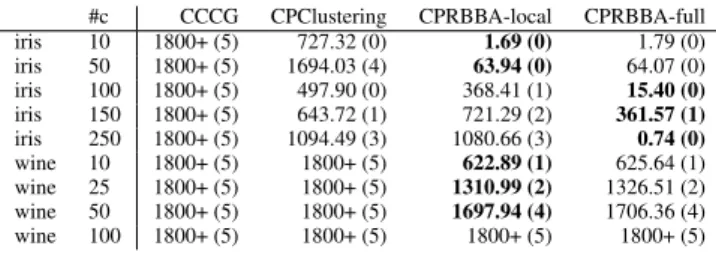
CL constraints only.The results for cannot-link constraints are shown in Table 4. Adding CL constraints can make the problem much harder. Here too CPRBBA outperforms the others, which is in line with the time difference in the unconstrained case. As more con-straints are added, an optimal solution can be found in the given time-out for fewer sampled constraint sets (see number between brackets), leading to higher average runtimes.

#c CCCG CPClustering CPRBBA-local CPRBBA-full iris 10 1800+ (5) 727.32 (0) 1.69 (0) 1.79 (0) iris 50 1800+ (5) 1694.03 (4) 63.94 (0) 64.07 (0) iris 100 1800+ (5) 497.90 (0) 368.41 (1) 15.40 (0) iris 150 1800+ (5) 643.72 (1) 721.29 (2) 361.57 (1) iris 250 1800+ (5) 1094.49 (3) 1080.66 (3) 0.74 (0) wine 10 1800+ (5) 1800+ (5) 622.89 (1) 625.64 (1) wine 25 1800+ (5) 1800+ (5) 1310.99 (2) 1326.51 (2) wine 50 1800+ (5) 1800+ (5) 1697.94 (4) 1706.36 (4) wine 100 1800+ (5) 1800+ (5) 1800+ (5) 1800+ (5)

Table 4. Runtimes averaged over 5 random samples of #c cannot-link constraints; between brackets number of runs that

timed-out (counted as 1800 seconds in average).

These results extend to the combination of must-link and cannot-link constraints (not shown).

Cluster-level constraints Table 5 shows runtimes for different datasets when adding a minimal or a maximal cluster size constraint. We can see that CPRBBA can handle such constraints well, and better than CPClustering. CPRBBA-full considers more constraints than CPRBBA-local in between iterations, and can hence provide tighter bounds. However, we observe that for some datasets, obtain-ing tighter bounds requires more search in one iteration to get them, thus loosing the benefits of the tighter bounds in subsequent itera-tions, and thus leading to overhead. For the iris dataset, the effort of searching for a tighter bound does pay of in the experiments. We observe similar results for a maximum cluster size constraint.

K min size cpclus. cprbba-local cprbba-full

ruspini 4 17 1.08 0.02 1.17 ruspini 4 18 270.00 9.00 24.06 soybean 4 10 1.28 1.39 1.78 soybean 4 11 1800+ 1563.12 1652.13 iris 3 38 564.86 1.32 1.67 iris 3 42 693.38 9.23 2.45 iris 3 46 933.23 341.23 18.46 iris 3 50 1508.77 1800+ 294.75

K max. size cpclus. cprbba-local cprbba-full

ruspini 4 20 0.54 0.01 0.05 ruspini 4 19 1800+ 602.82 794.83 soybean 4 14 1.28 1.32 1.83 soybean 4 13 17.52 13.19 17.44 iris 3 62 589.92 1.31 1.67 iris 3 58 723.63 3.95 3.04 iris 3 54 973.09 96.78 18.31 iris 3 50 1483.88 1800+ 158.75

Table 5. Runtime in seconds for clustering with minimum (top) and maximum (bottom) size constraint

6.3

Multi-Objective Constrained Clustering

Constraints offer a way to find solutions that better fit the problem at hand. Changing the objective function is another way. Curiously, whereas the aim of clustering is to find homogeneous as well as well-separated clusters, most measures, including WCSS, express only homogeneity. One solution is to use multi-objective optimization, with one measure for homogeneity and one for well-separatedness. The result is a set of Pareto optimal solutions, where a Pareto opti-mal solution is one for which it is not possible to improve the value of one criterion without degrading the value of the other one.

We propose an algorithm (Algorithm 4) to compute an exact set of Pareto solutions for bi-objective WCSS/Split optimization, so as to obtain both homogeneous and well-separated clusterings. It is based on the-constraintalgorithm [22] and is applicable to any complete method that can optimize WCSS under must-link constraints. In this algorithm, constrained single objective optimization (WCSS) is iter-ated, each time with a condition on the best value of the other objec-tive (minimal split) found so far. This minimal-split constraint can in turn be translated into must-link constraints.

Algorithm 4:Bi-objective WCSS/Split 1 Pareto sols← ∅

2 min split←0 3 repeat

4 ∆←Minimize WCSS(O,{Split >min split}) 5 min split←Split(∆)

6 if∆is not dominated in Pareto solsthen 7 Pareto sols←Pareto sols∪ {∆}

8 untilno∆was found;

In [12, 28, 27] the problem of finding the Pareto optimal solutions for minimizing the maximal diameter of the clusters and maximizing the minimal split between clusters is addressed, but without constraints. To our best knowledge the only work that handles user-constraints inside a multi-objective clustering problem is [8]. That work does not consider the WCSS criterion, and the criteria used often lead to thousands of equivalent clusterings corresponding to each Pareto point. Algorithm 4 can be easily modified to incorporate user-constraints, in case the Minimize WCSS algorithm supports it: another set of user-constraints can simply be added to the split con-straint at line 4.

Experiments Table 6 presents runtimes in seconds, number of Pareto solutions and the maximal number of clusterings ∆0 corresponding to each Pareto solution ∆ (i.e. W CSS(∆0) = W CSS(∆) and Split(∆0) = Split(∆)). We can see here (last column) that for each Pareto solution, there is always only one corre-sponding clustering, which contrasts with the thousands of equivalent solutions found in [8] for the Diameter/Split measure.

K time (s) #sols #c/s ruspini 4 0.01 1 1 soybean 4 1.58 4 1 hatco 4 32.52 24 1 hatco 5 1979.38 22 1 iris 3 1.11 10 1 wine 3 100.58 9 1 seeds 3 178.62 17 1

Table 6. Runtime, # Pareto solutions, maximal number of clusterings for each Pareto solution

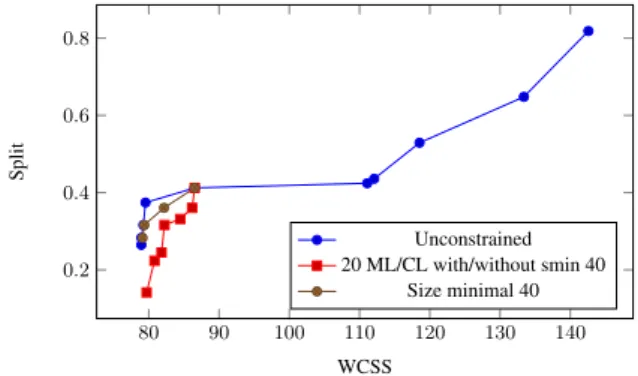
Our framework can also be used for bi-objective WCSS/Split un-der user constraints. To the best of our knowledge, it is the first method to support this bi-criterion optimization both for instance-and cluster-level constraints. Table 7 shows the results for differ-ent use cases on the Iris dataset. For four of these cases, the exact Pareto fronts are shown in Figure 1 (the two cases for 20 ML/CL constraints with and without the minimal size constraint have the

same Pareto front). We can see here the interest of being able to han-dle user-constraints during the optimization process. Indeed, in this dataset, each ground truth cluster is of size 50, whereas in the un-constrained use case, the Pareto solutions can give clusterings with unbalanced clusters. For instance, the last point in the Pareto front corresponds to a clustering with clusters of size 2, 50 and 98. The constrained cases have the last Pareto solution with WCSS=86.5396 and Split=0.412311. This solution is common to all the 4 cases, and the only corresponding clustering has clusters of size 49, 50, 51.

Use case time (s) #sols #c/s

unconstrained 1.11 10 1 20 ML/CL 13.68 7 1 40 ML/CL 9.66 8 1 size minimal 38 1.6 7 1 size minimal 40 1.8 4 1 20 ML/CL, size min 40 13.80 7 1 40 ML/CL, size min 40 9.75 8 1

Table 7. Results on Iris for bi-criterion constrained clustering cases

80 90 100 110 120 130 140 0.2 0.4 0.6 0.8 WCSS Split Unconstrained 20 ML/CL with/without smin 40 Size minimal 40

Figure 1. Pareto fronts for different cases on Iris

7

CONCLUSION

In this paper, we address one of the most popular constrained clustering task, the constrained minimum sum-of-squares clustering (MSSC). We extend the Repetitive Branch-and-Bound Algorithm, one of the best method for MSSC without user constraints, to inte-grate user constraints. The framework we propose is based on Con-straint Programming (CP), which is used in each internal branch-and-bound step, as well as in the computation of upper and lower bounds. We propose two different CP models in order to have tight lower bounds and construct a specific propagation mechanism to make better use of the computed bounds. Experiments on classic datasets show that our approach, even though being generic, is com-petitive compared to a dedicated implementation of RBBA in the un-constrained case. For un-constrained cases, our approach outperforms the existing state-of-the-art exact approaches. Furthermore, we show how its generality allows it to be used in a bi-objective constrained clustering setting.

To further enhance the efficiency of the framework, one may have to consider other ordering heuristics, including dynamic ones. More-over, RBBA has been applied to clustering tasks with other optimiza-tion criteria such as WCSD, to which our approach can be extended as well. Our bi-objective approach can also be used with non-exact constrained clustering methods, though the resulting Pareto front will be an approximation. Lastly, a mix of Russian Doll Search and our approach may lead to advances for both valued CSPs and clustering.

REFERENCES

[1] Daniel Aloise, Amit Deshpande, Pierre Hansen, and Preyas Popat, ‘NP-hardness of Euclidean Sum-of-squares Clustering’,Machine Learning, 75(2), 245–248, (2009).

[2] Daniel Aloise and Pierre Hansen, ‘An branch-and-cut SDP-based algo-rithm for minimum sum-of-squares clustering’,Pesquisa Operacional, 29(3), 503–516, (2009).

[3] Daniel Aloise, Pierre Hansen, and Leo Liberti, ‘An improved column generation algorithm for minimum sum-of-squares clustering’, Mathe-matical Programming,131(1-2), 195–220, (2012).

[4] Behrouz Babaki, Tias Guns, and Siegfried Nijssen, ‘Constrained clus-tering using column generation’, inProceedings of the 11th Interna-tional Conference on Integration of AI and OR Techniques in Constraint Programming for Combinatorial Optimization Problems, pp. 438–454, (2014).

[5] Michael J. Brusco, ‘An enhanced branch-and-bound algorithm for a partitioning problem’,British Journal of Mathematical and Statistical Psychology,56(1), 83–92, (2003).

[6] Michael J. Brusco, ‘A repetitive branch-and-bound procedure for min-imum within-cluster sums of squares partitioning’, Psychometrika, 71(2), 347–363, (2006).

[7] Thi-Bich-Hanh Dao, Kanh-Chuong Duong, and Christel Vrain, ‘A Declarative Framework for Constrained Clustering’, inProceedings of the European Conference on Machine Learning and Principles and Practice of Knowledge Discovery in Databases, pp. 419–434, (2013). [8] Thi-Bich-Hanh Dao, Khanh-Chuong Duong, and Christel Vrain,

‘Con-strained clustering by constraint programming’,Artificial Intelligence, DOI: 10.1016/j.artint.2015.05.006, (2015).

[9] Thi-Bich-Hanh Dao, Khanh-Chuong Duong, and Christel Vrain, ‘Con-strained minimum sum of squares clustering by constraint program-ming’, inPrinciples and Practice of Constraint Programming, CP 2015, Proceedings, pp. 557–573, (2015).

[10] Ian Davidson and S. S. Ravi, ‘Clustering with Constraints: Feasibility Issues and the k-Means Algorithm’, inProceedings of the 5th SIAM International Conference on Data Mining, pp. 138–149, (2005). [11] Ian Davidson, S. S. Ravi, and Leonid Shamis, ‘A SAT-based

Frame-work for Efficient Constrained Clustering’, inProceedings of the 10th SIAM International Conference on Data Mining, pp. 94–105, (2010). [12] M. Delattre and P. Hansen, ‘Bicriterion cluster analysis’,IEEE Trans.

Pattern Anal. Mach. Intell., (4), 277–291, (1980).

[13] O. du Merle, P. Hansen, B. Jaumard, and N. Mladenovic, ‘An interior point algorithm for minimum sum-of-squares clustering’,SIAM Jour-nal on Scientific Computing,21(4), 1485–1505, (1999).

[14] A. W. F. Edwards and L. L. Cavalli-Sforza, ‘A method for cluster anal-ysis’,Biometrics,21(2), 362–375, (1965).

[15] T. Gonzalez, ‘Clustering to minimize the maximum intercluster dis-tance’,Theoretical Computer Science,38, 293–306, (1985).

[16] Pierre Hansen and Brigitte Jaumard, ‘Cluster analysis and mathematical programming’,Mathematical Programming,79(1-3), 191–215, (1997). [17] Robert E. Jensen, ‘A dynamic programming algorithm for cluster anal-ysis’,Journal of the Operations Research Society of America,7, 1034– 1057, (1969).

[18] W. L. G. Koontz, P. M. Narendra, and K. Fukunaga, ‘A branch and bound clustering algorithm’,IEEE Trans. Comput.,24(9), 908–915, (1975).

[19] Marianne Mueller and Stefan Kramer, ‘Integer Linear Programming Models for Constrained Clustering’, inProceedings of the 13th Inter-national Conference on Discovery Science, pp. 159–173, (2010). [20] Dan Pelleg and Dorit Baras, ‘K-means with large and noisy constraint

sets’, inMachine Learning: ECML 2007, volume 4701 ofLecture Notes in Computer Science, pp. 674–682. Springer Berlin Heidelberg, (2007). [21] Douglas Steinley, ‘k-means clustering: A half-century synthesis’,

British Journal of Mathematical and Statistical Psychology,59(1), 1– 34, (2006).

[22] Vincent T’kindt and Jean-Charles Billaut, Multicriteria Scheduling, Theory, Models and Algorithms, Springer, 2nd edn., 2005.

[23] B.J. van Os and J.J. Meulman, ‘Improving Dynamic Programming Strategies for Partitioning’,Journal of Classification, (2004). [24] G´erard Verfaillie, Michel Lemaˆıtre, and Thomas Schiex, ‘Russian doll

search for solving constraint optimization problems’, inProceedings of the Thirteenth National Conference on Artificial Intelligence and Eighth Innovative Applications of Artificial Intelligence Conference, AAAI 96, pp. 181–187, (1996).

[25] K. Wagstaff and C. Cardie, ‘Clustering with instance-level constraints’, inProceedings of the 17th International Conference on Machine Learn-ing, pp. 1103–1110, (2000).

[26] Kiri Wagstaff, Claire Cardie, Seth Rogers, and Stefan Schr¨odl, ‘Con-strained K-means Clustering with Background Knowledge’, in Pro-ceedings of the 18th International Conference on Machine Learning, pp. 577–584, (2001).

[27] J. Wang and J. Chen, ‘Clustering to maximize the ratio of split to diam-eter’, inProceedings of the 29th International Conference on Machine Learning, (2012).

[28] Y. Wang, H. Yan, and C. Sriskandarajah, ‘The weighted sum of split and diameter clustering’,Journal of Classification,2(12), 231–248, (1996). [29] Y. Xia and J. Peng, ‘A cutting algorithm for the minimum