Risk-Based Maintenance Planning Model for
Oil and Gas Pipelines
Laya Parvizsedghy
A Thesis
In the Department
of
Building, Civil and Environmental Engineering
Presented in Partial Fulfillment of the Requirements
For the Degree of
Doctor of Philosophy (Civil and Environmental Engineering) at
Concordia University
Montreal, Quebec, Canada
October 2015
CONCORDIA UNIVERSITY
SCHOOL OF GRADUATE STUDIES
This is to certify that the thesis prepared
By: Laya Parvizsedghy
Entitled: Risk-Based Maintenance Planning Model for Oil and Gas Pipelines
and submitted in partial fulfillment of the requirements for the degree of
DOCTOR OF PHILOSOPHY (Building Engineering)
complies with the regulations of the University and meets the accepted standards with respect to originality and quality.
Signed by the final examining committee:
Dr. I. Stiharu Chair
Dr. R. Sadiq External Examiner
Dr. G. Gopakumar External to Program
Dr. O. Moselhi Examiner
Dr. Z. Zhu Examiner
Dr. T. Zayed Thesis Supervisor
Approved by:
ABSTRACT
Risk-Based Maintenance Planning Model for Oil and Gas Pipelines Laya Parvizsedghy, PhD
Concordia University, 2015
Oil and gas pipelines are the main means of transporting fossil fuels from the wellheads and processing facilities to the distribution centers. The 2013 US infrastructure report card assigned a grade of D+ to energy pipelines signifying they are in a poor condition. More than 10,000 incidents were reported on oil and gas pipelines during the last two decades, most of which resulted in considerable consequences. Recent failures and ruptures have raised concerns over the risk of failure of such pipes in Canada. The main objective of this research is to develop a risk-based maintenance planning model for oil and gas pipelines. The research develops a probability of failure (POF) and a consequence of failure (COF) prediction model and establishes a risk-based inspection and simulation-based rehabilitation planning models.
The POF model develops a comprehensive index by applying the granular theory of uncertainty and the principles of probability theory to forecast the POF of oil and gas pipes. The neuro-fuzzy technique is employed to develop a model that forecasts the financial consequences of the potential failures of such pipes. An integrated fuzzy risk evaluation model is developed with 25 fuzzy rules to assess a pipeline’s risk index. A fuzzy expert system is developed to select the inspection tools and determine their run-frequency according to the failure risk of a pipeline. Regression analysis is applied to develop a risk growth profile to forecast the maximum failure risk of various inspection scenarios. Scenarios are ranked based on their risk-cost index, which integrates two main
indices: 1) maximum risk of failure, and 2) life cycle cost of scenarios, computed by applying the Monte-Carlo simulation. Finally, a comprehensive maintenance model proposes the optimum maintenance plans with the lowest LCC, developing a third-degree risk-based deterioration profile of the pipelines.
The POF model’s sensitivity results highlight that cathodic protection effectiveness and soil resistivity are the leading causes of external corrosion failures, while the depth of cover is an important factor of mechanical damages. The COF model attests that diameter, as well as the location properties are important factors for estimating the financial consequences. The developed risk assessment model is validated using a test dataset that proved the models are accurate with about 80% validity. The developed models are applied on a case study of a 24-inch pipe. The POF and COF of the pipe are computed, and the results suggest that the pipe’s risk index is above medium with an average index of 3.5. The study proposes the application of an inspection tool, which decreases the risk growth by 50% during the service life of the pipeline. The application of the maintenance planning model proposes a combination of recoat, repair, and replacement with a medium size of rehabilitation. The net present value of the proposed scenario of maintenance is estimated to cost around 1.7 million dollars over the life cycle of the pipeline, compared to the last-ranked alternative that costs over three million dollars. This research offers a framework to develop a comprehensive index to predict the failure risk of pipes using historical data that can be extended to the other infrastructure types. It develops a model to plan for the optimal pipeline maintenance, and provides an overall image of its service life. The developed models will help the operators predict the risk of failure and plan appropriately for the life cycle of their oil and gas pipelines.
ACKNOWLEDGEMENT
I would like to express my highest gratitude to my supervisor, Professor Tarek Zayed, for his invaluable supervision and continuous support during my PhD studies. His patience and positive attitude along with exceptional insights made me capable of walking through this interesting but challenging journey.
In addition, I would like to express my special gratitude to Prof. Osama Moselhi for his great mentorship. I also acknowledge for the constructive feedback of the members of my Ph.D. examining committee including Dr. Zhenhua Zhu, Dr. Govind Gopakumar and Dr. Rehan Sadiq. I express my special acknowledgments to Prof. Oscar Pekau for his endless support in offering his time and advice during and after his very interesting Ph.D. seminar course.
I also acknowledge the helpful comments and support of my friends and colleagues at the Construction Automation Lab. I had the opportunity to work in a professional and friendly environment. I express my appreciation to the senior safety engineer, Dr. Naser Badri, who devoted his valuable time to discuss various aspects of my research.
Last but not least, I am deeply grateful to my family for their unconditional support and encouragement.
To all of those who provide humanitarian aid
to the people in need.
TABLE OF CONTENTS
LIST OF FIGURES ... xi
LIST OF TABLES ... xv
CHAPTER 1: INTRODUCTION ... 1
1.1 Problem Statement and Research Motivation ... 1
1.2 Research Objectives ... 2
1.3 Research Methodology ... 2
1.4 Structure of the Thesis ... 5
CHAPTER 2: LITERATURE REVIEW ... 6
2.1 Introduction ... 6
2.2 Oil and Gas Pipelines ... 6
2.3 Risk Assessment ... 9
2.3.1 Definition of Risk Assessment... 9
2.3.2 Risk-Based Decision Support Models for Oil and Gas Pipelines ... 10
2.3.3 Sources of Failure ... 12
2.3.4 Probability of Failure ... 13
2.3.5 Consequences of Failure ... 27
2.4 Oil and Gas Pipelines’ Operation Phase ... 33
2.4.1 Inspection Methods ... 34
2.5.1 Bow-Tie analysis ... 41
2.5.2 Artificial Neural Networks (ANN) ... 45
2.5.3 Fuzzy Set Theory ... 49
2.7.3 General Theory of Uncertainty ... 51
2.5.4 Neuro-fuzzy ... 52
2.5.5 Monte Carlo Simulation ... 55
2.6 Findings, Limitations, and Research Gap ... 56
CHAPTER 3: RESEARCH METHODOLOGY ... 58
3.1 Overall Research Methodology ... 58
3.2 Risk Assessment Model ... 60
3.2.1 Identification of Failure Sources and Contributing Variables ... 60
3.2.2 Probability of Failure Model ... 66
3.2.3 Consequence of Failure Model ... 76
3.2.4 Validation of the POF and COF Models... 89
3.2.5 Integrated fuzzy risk evaluation model ... 90
3.3 Maintenance Model ... 93
3.3.1 Inspection Planning ... 93
3.3.2 Rehabilitation Planning Model ... 100
CHAPTER 4: DATA COLLECTION ... 105
4.2 Frequency of Failures in Monetary Consequence Classes ... 116
4.3 Rehabilitation Cost Data ... 120
CHAPTER 5: MODEL DEVELOPMENT AND IMPLEMENTATION ... 123
5.1 Bow-Tie ... 125
5.2 Probability of Failure Prediction Model ... 128
5.2.1 Data Analysis and Model Implementation ... 130
5.2.2 Sensitivity Analysis ... 141
5.2.3 Validation of the Developed Model ... 143
5.3 Consequences of Failure Prediction Model ... 145
5.3.1 Consequences of Failure Model Validation ... 152
5.4 Integrated Fuzzy Risk Index ... 153
5.5 Inspection Planning ... 155
5.6 Rehabilitation Planning Model ... 163
5.6.1 Overall Scenarios ... 167
5.5.2 Economic Parameters... 168
5.7 Model Implementation to a Case Study ... 169
5.8 Automation of the developed model ... 182
CHAPTER 6: CONCLUSIONS AND RECOMMENDATIONS ... 188
6.1 Summary and Conclusions ... 188
6.3 Research Limitations ... 192
6.4 Future Work and Recommendations ... 192
6.4.1 Enhancement Areas ... 193
6.4.2 Extension Areas ... 194
REFERENCES ... 195
Appendix (A): Developed indices to calculate the POF of pipes ... 205
Appendix (B): Sample probability distribution functions for POF model ... 212
LIST OF FIGURES
Figure 2- 1: Components of Natural Gas Pipelines Network (GAO 2000) ... 8
Figure 2- 2: Oil and Gas Pipelines Fault Tree (Shahriar et al. 2012) ... 22
Figure 2- 3: Oil and Gas Pipelines Fault Tree; part A (Shahriar et al. 2012) ... 23
Figure 2- 4: Oil and Gas Pipelines Fault Tree; part B (Shahriar et al. 2012) ... 23
Figure 2- 5: Event Tree Diagram of Natural Gas Pipelines (Shahriar et al. 2012) ... 32
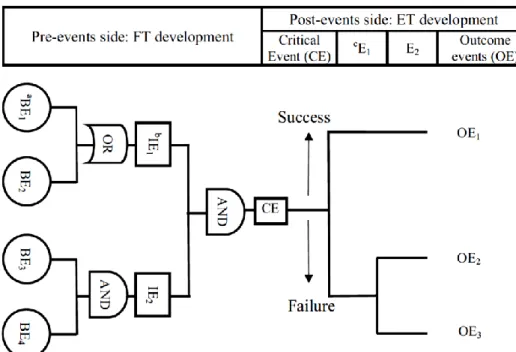
Figure 2- 6: Generic Bow-tie Model (adapted from Dianous & Fievez 2006) ... 42
Figure 2- 7: Elements of a Bow-tie model (adapted from Ferdous et al. 2012) ... 43
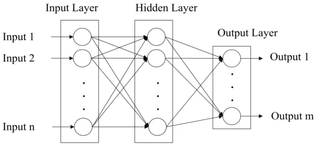
Figure 2- 8: Typical Artificial Neural Network (Parvizsedghy and Zayed 2013) ... 47
Figure 2- 9: Application of granular theory to a distribution function ... 51
Figure 2- 10: First Order Sugeno fuzzy model ... 53
Figure 2- 11: ANFIS architecture ... 53
Figure 3- 1: Overall Model Flowchart ... 59
Figure 3- 2: Overall Flow of Identification Phase ... 60
Figure 3- 3: Classifications of Identified Risk Factors ... 62
Figure 3- 4: Identified factors affecting each failure type ... 65
Figure 3- 5: Flowchart to develop the probability of failure model ... 67
Figure 3- 6: Modified sample fault tree ... 69
Figure 3- 7: Model Development Process ... 77
Figure 3- 8: Mamdani Fuzzy Inference System (Mathworks 2013) ... 86
Figure 3- 9: Sample FIS structure with four input variables (Mathworks 2013)... 87
Figure 3- 10: Sample fuzzy inference structure and output rules ... 88
Figure 3- 12: Inspection planning model ... 94
Figure 3- 13: Risk-based inspection model development ... 97
Figure 3- 14: Rehabilitation planning model development flowchart ... 101
Figure 4- 1: Distribution of Failure Sources (1986-2013) ... 107
Figure 4- 2: Air temperature map of North America in January 2011 (NOAA 2015) ... 109
Figure 4- 3: Mean air temperature of Texas State in January 2010 (NOAA 2015) ... 110
Figure 4- 4: Mean soil moisture content values for Texas State in December 2014 ... 110
Figure 4- 5: Wind speed map for Texas State in December 2014 ... 111
Figure 4- 6: Frequency of Failure Sources versus Age Classes (1986-2013)... 112
Figure 4- 7: Frequency of Failure Sources versus Diameter Classes (1986-2013) ... 113
Figure 4- 8: Frequency of Failure Sources versus Pipe wall Thickness Classes (1986-2013) ... 113
Figure 4- 9: Frequency of Failure Sources versus Pipe Maximum Operating Pressure (MOP) Classes (1986-2013) ... 114
Figure 4- 10: Frequency of Failure Sources versus SMYS Classes (1986-2013) ... 115
Figure 4- 11: Frequency of Failure Sources versus Coating Types (2010-2013) ... 115
Figure 4- 12: Frequency of Age Classes versus Monetary Consequence Classes (1986-2013) ... 116
Figure 4- 13: Frequency of Diameter Classes versus Monetary Consequence Classes (1986-2013)... 117
Figure 4- 14: Frequency of Wall Thickness Classes versus Monetary Consequence Classes (1986-2013)118Figure 4- 15: Frequency of MOP Classes versus Monetary Consequence Classes (1986-2013) ... 119
Figure 4- 16: Frequency of SMYS Classes versus Monetary Consequence Classes
(1986-2013) ... 119
Figure 5- 1: Model development and implementation overall process... 124
Figure 5- 2: Bow-Tie model (Fault tree part) ... 127
Figure 5- 3: Event tree part of Bow-tie model ... 128
Figure 5- 4: PDFs associated with A: pH, B: SR, and C: RP historical data ... 129
Figure 5- 5: Sensitivity analysis results ... 142
Figure 5- 6: Validation results ... 144
Figure 5- 7: Actual versus Predicted POF in the testing dataset ... 145
Figure 5- 8: Structure of the Model ... 149
Figure 5- 9: Membership function generated for input variables ... 150
Figure 5- 10: Three dimensional sensitivity surfaces ... 152
Figure 5- 11: Risk index model fuzzy rules ... 154
Figure 5- 12: Risk Index surface demonstration ... 155
Figure 5- 13: Membership functions of Fuzzy Inspection Tool Selection Model ... 159
Figure 5- 14: Surfaces demonstration of the Fuzzy Inspection Tool Selection Model .. 159
Figure 5- 15: Cumulative risk growth profile ... 160
Figure 5- 16: Fuzzy membership functions of the inspection tools’ detection capability ... 161
Figure 5- 17: Cumulative after inspection risk profile of an example pipeline ... 162
Figure 5- 18: EUAC Result of Monte Carlo simulation ... 162
Figure 5- 19: Risk-based deterioration profile ... 165
Figure 5- 21: Calculated mean values of POF with respect to all ... 170
Figure 5- 22: Estimated consequences of failure for all failure sources ... 171
Figure 5- 23: Risk growth Profile for ROCOMBO MFL-A/XT ... 175
Figure 5- 24: Sample Deterioration Profiles ... 176
Figure 5- 25: Simulation-Based EUAC Amounts (Sorted based on NPV, Most Likely)179 Figure 5- 26: Simulation- Based NPV Amounts ... 180
Figure 5- 27: Sample Excel sheet calculation for Internal Corrosion Failures ... 182
Figure 5- 28: Sample COF calculation sheet ... 183
Figure 5- 29: Sample risk score calculation of the case study ... 184
Figure 5- 30: Fuzzy inspection tool selection model demonstration ... 185
Figure 5- 31: Sample calculation sheet for life cycle cost analysis of rehabilitation scenarios ... 186
LIST OF TABLES
Table 2- 1: Failure types in six various sources ... 13
Table 2- 2: Probability Assessment Scale (Infraguide 2006) ... 14
Table 2- 3: Failure Probability Scale of Assessment (DNV 2010) ... 14
Table 2- 4: Summary of the variables affecting the probability of corrosion failures ... 24
Table 2- 5: Summary of the variables affecting the probability of operational failures ... 25
Table 2- 6: Summary of the variables affecting the probability of external failures ... 26
Table 2- 7: Safety consequences scale (Adapted from: DNV 2010) ... 27
Table 2- 8: Environmental consequences scale (Adapted from: DNV 2010a) ... 28
Table 2- 9: Economic consequences scale (Adapted from: DNV 2010a) ... 28
Table 2- 10: Different operation elements (Parvizsedghy et al. 2014) ... 34
Table 2- 11: Recommended Types of Rehabilitation for Different Types of Defects (Parvizsedghy et al. 2014) ... 35
Table 2- 12: Major categories of inspection to monitor various failure types (Hopkins et al. 2000) ... 36
Table 2- 13: Major Assessment Methods (Adapted from: Thompson 2000) ... 37
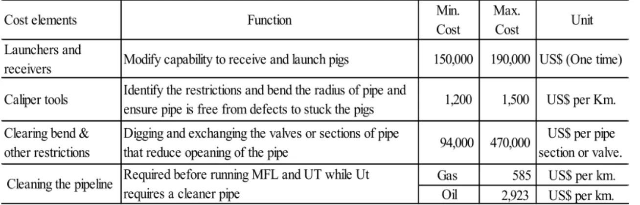
Table 2- 14: Cost elements of Pipeline Preparation for ILI (Adapted from: Thompson 2000) ... 38
Table 2- 15: Summary of application of inspection tools (INGAA 2007; NACE 2002) . 39 Table 2- 16: Description and shapes of Graphical symbols used in Fault tree models (adapted from Ferdous 2006) ... 44
Table 2- 17: Parameters of back-propagation method (Hegazy et al. 1994) ... 48
Table 3- 2: Variables used in the numerical models developed for the failure consequence
prediction models ... 81
Table 3- 3: Primary input variables ... 83
Table 3- 4: Probability of failure scale of evaluation ... 91
Table 3- 5: Sample list of inspection techniques and their cost and recommended range of operation frequency ... 94
Table 3- 6: Sample index of inspection frequency based on the level of failure probability ... 95
Table 4- 1: Sample data excel sheet (PHMSAa 2014) ... 106
Table 4- 2: Cost Data for Different Types of Rehabilitation Techniques (US $) ... 121
Table 5- 1: Coating types categories ... 130
Table 5- 2: Categories defined for the basic causes ... 133
Table 5- 3: Contribution of the identified basic causes to the EC failures ... 135
Table 5- 4: Contribution of the pipe diameter categories on EC, IC and MW failure sources... 137
Table 5- 5: Contribution coefficients of the installation year categories all failure sources ... 137
Table 5- 6: Diameter-based adjustment factors for all failure sources ... 138
Table 5- 7: Indices related to probability of after-failure events for oil pipes ... 140
Table 5- 8: Financial consequence levels description ... 146
Table 5- 9: Sample entry data ... 147
Table 5- 10: Results of Neuro-fuzzy tested networks ... 148
Table 5- 12: Validation results of the final model ... 153
Table 5- 13: Inspection methods applied for external corrosion failures ... 157
Table 5- 14: Frequency range of Inline inspection application for oil and gas pipelines with respect to their level of failure probability ... 157
Table 5- 15: Inspection tool selection versus failure consequence level ... 158
Table 5- 16: Defects Size Scale for Various Rehabilitation Techniques (meters) ... 163
Table 5- 17: Condition Increments for Different Types of Rehabilitation ... 164
Table 5- 18: Pipeline Condition Thresholds for Rehabilitation Techniques ... 167
Table 5- 19: Overall Scenario Types ... 168
Table 5- 20: Primary data of case study... 170
Table 5- 21: Risk parameters and Risk indices of the case study ... 172
Table 5- 22: Frequency determination and Inspection tool selection for case study ... 173
Table 5- 23: Detection capability level for the selected inspection tools ... 173
Table 5- 24: Calculated indices for each inspection tool ... 174
Table 5- 25: Maximum risk, EUAC and Risk-Cost indices of the inspection scenarios 174 Table 5- 26: Scenarios Sorted Based on Simulation-Based NPV (US $) ... 179
Table 5- 27: Case Study Maintenance Plan ... 181
Table A- 1: Contribution of basic causes to IC and MW failures ... 206
Table A- 2: Contribution of the identified basic causes to the MD failures ... 207
Table A- 3: Contribution of the identified basic causes to IO and NF ... 208
Table A- 4: Contribution of the pipe diameter categories to MD, IO and NF failure sources... 210
Table B- 1: Distribution functions associated with soil corrosion ... 212 Table B- 2: Distribution functions associated with diameter categories of Gas Onshore Pipes ... 213 Table B- 3: Distribution functions associated with installation year categories of gas onshore pipes ... 214 Table C- 1: Data fields on Gas transmission and Gathering Pipes (2010-2015) ... 215
CHAPTER 1: INTRODUCTION
1.1 Problem Statement and Research MotivationWhile pipelines are considered to be the safest and most efficient way to transport hazardous liquids and natural gas, there is still a probability of failure, with economic, safety and damaging ecological consequences. The Pipeline and Hazardous Materials
Safety Administration (PHMSAa 2014) of the US has gathered and published data on the
oil and gas pipeline failures since 1970. Over 10,000 failures were recorded from 1993 to 2013 in the US, which resulted in six billion dollars of property damages and the leakage of around 2.3 million barrels of hazardous liquids into the environment. The records also indicate that 377 fatalities and 1,489 serious injuries occurred during this period. These figures underscore why the assessment of oil and gas pipelines deserves serious attention. In addition, owners or operators of such pipelines must develop and implement an integrity management program as mandated by Canadian Pipeline regulatory. Whereas the Guidelines for Pipeline Integrity Management Programs (Annex N) only provides an overall approach to mitigate risk of failures of the pipelines during the operation phase (CSA 2003).
The failure of oil and gas pipelines has been extensively addressed in the literature, however the studies conducted to-date suffer from several limitations. These research works have either focused on a single type of failure, e.g. corrosion or third-party activities, or they have developed subjective models. Physical models rely on analyzing inline inspection data, which is very expensive to gather and does not even exist in the early stages of a pipeline’s operation. In addition, some pipes are not piggable. The
existing statistical models do not consider the specific properties of pipes in forecasting the probability and consequences of their failure. Moreover, there is no structured method with which to plan for the inspection and rehabilitation of pipes. Therefore, the current state-of-the-practice is not mature enough to fully support oil and gas operators in the decision-making process.
This study aims to develop an objective quantitative model on the failure assessment of oil and gas pipelines, a model that can also be used to plan maintenance solutions. The result of this research will help oil and gas pipeline operators in their decision-making process for inspection and maintenance plans.
1.2 Research Objectives
The main objective of this research is to develop a risk-based maintenance decision support model for oil and gas pipelines during the operation phase. This objective can be broken down into the following sub-objectives:
1. Identify and study the sources of failure and their effects on oil and gas pipelines; 2. Predict the failure probability of such pipes;
3. Develop a consequence of failure assessment model;
4. Develop an integrated risk evaluation model;
5. Establish a risk-based inspection planning model; and 6. Develop a deterioration-based rehabilitation planning model.
1.3 Research Methodology
A comprehensive description of the methodology developed in this research is presented in chapter 3. A summary of the research methodology is presented in the following steps:
Step 1: Literature Review
The literature is reviewed to find those works that are most relevent to the risk assessment and maintenance of oil and gas pipelines. The literature review also includes an evaluation of the techniques that can be used in the model development.
Step 2: Build a Bow-tie model
A Bow-tie model is applied to develop the graphical representation of the variables that contribute to failure and to show their relationship to the major consequences of the failure. This approach includes two main parts; a fault tree and an event tree. Due to the complexity of oil and gas pipeline behaviour, this is a useful technique with which to elaborate on the causes and after-failure events of pipeline failure. Finally, this step provides a comprehensive view of the pipeline failure scenarios.
Step 3: Probability of Failure Model
The failure probability is assessed based on the bow-tie model, and the contribution of each category of contributing causes is calculated using the historical data from pipeline incidents. The model then computes the failure probability based on the causes of incidents and measures the probability of the occurrence of each major consequence. The model produces all the indices and equations required to compute the absolute probability of failure.
Step 4: Consequences of Failure Model
This model predicts the monetary consequence level of various pipeline failure scenarios. The neuro-fuzzy technique is used to develop this model, utilizing data gathered from the history of pipeline incidents in the US. This technique is a powerful pattern
recognition tool,recognising the relationship between the input and output variables. Compared to using regression and artificial neural networks it develops a more accurate and robust model.
Step 5: Integrated Fuzzy Risk Evaluation Model
A fuzzy expert system that integrates the probability of failure with the consequences of failure is developed to evaluate the failure risk level. A fuzzy inference system is developed; its rules defined based on the existig risk matrices and expert opinions.
Step 6: Risk-Based Inspection Planning
The appropriate pipeline inspection techniques are selected and their optimal run frequency of running is proposed. This is performed according to the afore-calculated probabilities of failure and consequences. Various inspection scenarios are developed based on the risk growth prediction profile. The inspection scenarios are ranked based on a newly introduced index, theRisk-Cost, which multiplies the maximum risk of failure by the life cycle cost.
Step 7: Maintenance planning
This step helps oil and gas pipeline operators develop appropriate maintenance scenarios for the pipelines in their network. The rehabilitation scenarios are offered via the prediction of the deterioration profile, and then the required rehabilitation techniques are determined based on the deterioration profile. The Life Cycle Costs (LCCs) of the generated scenarios are calculated using Monte Carlo simulation. Accordingly, the scenarios with the lowest LCCs indicate the associated optimum pipeline maintenance plans.
1.4 Structure of the Thesis
This thesis is comprised of six chapters, summarised as follows:
Chapter 1 highlights the problem statement and the research motivation. The research objectives and the overall model framework are also presented in this chapter.
Chapter 2 reviews the previous works on failure and risk assessment of oil and gas pipelines. The literature review results are organised and the research gaps identified. In addition, the most-suitable techniques for this research are investigated.
Chapter 3 presents the research methodology in detail. It is composed of two distinctive models, a risk assessment model and a maintenance model. The risk assessment model contains three main steps: identification, failure probability assessment, and consequence evaluation. The maintenance model is composed of inspection planning and rehabilitation planning sub-models.
Chapter 4 explains the historical data gathered to develop the proposed models. It also includes an analysis of the historical data, divided into two main categories: (1) the frequency of failure sources associated with different variables and (2) monetary consequences classification.
Chapter 5 elaborates the development of the models based on the proposed methodology introduced in Chapter 3. It also elaborates on the implementation of the developed model for a 24-inch pipe. This chapter continues with an explanation of the semi-automated system.
Finally, Chapter 6 highlights the conclusions and the expected contributions of the research and some recommendations for future work.
CHAPTER 2: LITERATURE REVIEW
2.1 IntroductionThis chapter aims at providing a retrospective and comprehensive literature review of the risk assessment, maintenance solutions, and decision support models of oil and gas pipelines in the operation phase. It starts with an introduction to oil and gas pipelines and their types (Section 2.2). Then, a comprehensive review of the risk assessment researches including the general risk management methods and those related to the oil and gas pipelines is presented (Section 2.3). After that, the existing guidelines on various types of operations for the maintenance of such pipelines are introduced (Section 2.4). Finally, selected techniques that have the potential to be used in this research are reviewed, and the advantages and disadvantages of each are demonstrated (Section 2.5). At last, the limitations of the previous studies and overall finding of this review are presented (Section 2.6).
2.2 Oil and Gas Pipelines
Statistics proves that 24% of US energy consumption is provided by natural gas and another 39% from petroleum products. The pipelines network in the US transport almost all of the natural gas and around 65% of the hazardous liquid products. Pipelines are considered as the most practical and safest way of transporting these products. The pipeline network in the US consists of 2.5 million miles and includes three primary types according to their function as follows (PHMSAa 2014):
Gas transmission and gathering pipelines: There are approximately 320,000 miles of onshore and offshore transmission pipelines in the US. Gathering pipelines gather natural gas from wellheads and transmission pipelines carry products in large volumes from the processing facilities to the communities, power plants, and factories over long distances. These pipelines may range from 2 to 42 inches in diameter (PHMSAa 2014).
Gas distribution pipelines: There were around 2.1 million miles of distribution pipelines in 2001. They carried products from the processing facilities to the residential, commercial, and industrial customers. Gas distribution pipelines are also divided into two groups of main and service lines. Main lines are larger in diameter; while the service lines are from ½ to 2 inches in diameter (PHMSAa
2014).
Hazardous liquid pipelines: These pipelines cover 185,000 miles of the network.
They carry hazardous liquids from the wellheads to the customers. These pipelines are ranged from 2 to 42 inches in diameter. (PHMSAa 2014)
Figure 2.1 presents a schematic view of the network of oil and gas pipelines. The life cycle of these pipeline projects includes three main phases including design, construction, and operation. The main steps of pipeline construction are as followed (PHMSAa 2014):
1- Site Preparation 2- Pipe Stringing
3- Trenching
6- Coating
7- Lowering and Backfilling
8- Testing
9- Site Restoration
2.3 Risk Assessment
2.3.1 Definition of Risk Assessment
Failures have happened over the life of oil and gas pipelines; although, they are assumed the safest and more economic than the other methods of transporting the petroleum products. Risk assessment is a tool that can facilitate maintenance decision-making by forecasting the failures of oil and gas pipelines. Risk assessment guidelines have provided a definition of risk from various perspectives (Infraguide 2006, Dey 2009, and Dey 2010). Infraguide (2006) defined risk as a combination of the probability and the consequences of the scenarios that have adverse effects on the operation of different infrastructure types. Consequently, risk management aims to decrease the risk of failure and details this process in three main phases: Identification, Evaluation, and Mitigation planning of the risks.
DNV (2010) published a report about the recommended practice on risk assessment of third party sources of failures. The report defined sources of failure of pipelines as accidental events that can lead to the failure of the pipes, which was titled: the end-event. Then, it defined risk assessment as the evaluation of the frequency and consequences of the end-event. DNV (2009) developed recommendations on the integrity management of sub-sea pipelines. This study suggested selecting the activities in the operation phase of pipelines based on the risk assessment. Then, it specified the steps of the risk assessment process as are followed:
Identify risks and types of failures
Estimate risk of failure level (CoF × PoF)
2.3.2 Risk-Based Decision Support Models for Oil and Gas Pipelines
There has been an extensive effort in the previous studies to analyze and assess the risks of oil and gas pipelines and develop risk-based decision support systems for oil and gas pipes (Han & Weng 2010, Han & Weng 2011, Dey 2003, Dey 2004, Dey et al. 2004). A quantitative method was proposed by Han & Weng (2010) to evaluate the individual risks of natural gas pipeline networks. This method combined the probability of failures and their internal and external consequences. External effects included those of individual and societal while internal effects evaluated the monetary consequences. The model applied an overall rate of failure to calculate the probability of failure and multiplied it by a function of variables. Then, pipelines were classified into external and internal ones. For the former group, the individual and social consequences were computed. This part of the model focused on the safety related consequences and considered harms of a failure on gas pipelines. The coefficient of the pressure of the pipeline with the expected economic loss was multiplied by the pressure of the node that was vulnerable to fail to calculate the economic consequences. The failure rate was an average rate of incidents that was computed based on the historical data that was recorded through the historical data of failures on European gas pipeline network (EGIG 1999). The failure rate of all pipelines was considered equal unless the correction factor was applied; however, no function was developed to calculate this factor.
Han and Weng (2011) developed a model to compare the risk of failure of urban gas pipelines in a network. This model considered the causes of failures of such pipelines and calculated their weights based on the historical data. Frequency of the failures was
obtained to calculate the weight of importance of the causes of failure applying reliability engineering theory. Then, the probability of happening of each cause of failure was computed and multiplied by its related weight. The method was implemented on two pipelines and was compared with the results of a quantitative method proposed by Han and Weng (2010) to prove the validity of the developed model.
Dey (2003) evaluated the risk of failure of different segments of a cross-country pipeline and developed strategies for the selection of the inspection techniques for such pipelines. Risk-based decision-making support system was developed by Dey (2004) using Analytic Hierarchy Process (AHP) technique. This model applied expert opinion to obtain the weight of variables that were identified to contribute to the failure of pipelines. Variables were categorized as risk factors that included external and internal corrosion, construction and material defects, as well as acts of God.
Later, Dey et al. (2004) developed a risk-based maintenance model for offshore pipelines. After introducing likelihood and consequence loops of risks, expert opinion was obtained to calculate the relative weights of each factor of the loops applying AHP. Ranges of effect values from 1 to 10 were considered for assessing each factor. The model calculated the risk score of each pipeline by summing up the effect values multiplied by associated weights of the factors. Finally, one of the results was prioritizing assets of a network of pipelines. Most of the factors such as corrosion were evaluated subjectively; although, the research tried to minimize the subjectivity of the decision-making process in this problem. The model did not recognize the severity of different risks of failures. Consequently, inspection tools were proposed through an experience-based process,
a comprehensive model and needed the expertise to analyze and propose the best technique.
2.3.3 Sources of Failure
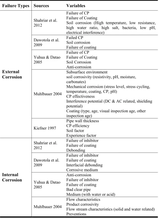
The first step in the risk assessment of infrastructures is to identify the risks associated with their failure (Infraguide 2006; DNV 2009 & 2010). There are different classifications of infrastructure risks. Sources of failures and defects that result in the failures of oil and gas pipelines have been the subject of grouping risks of failures (Shahriar et al. 2012, Dawotola et al. 2009, Yuhua & Datao 2005, and Muhlbauer 2004). This section details how previous works categorized the failures of oil and gas pipelines. Muhlbauer (2004) defined the risk of oil and gas pipelines as the loss of integrity and product. He also extended the risk definition to the failure of executing the intended functions by blockage, contamination or equipment failure. It was mentioned that leakage in most urban pipelines such as water, sewer, and urban gas distribution can tolerate some amount of leakage and would not be considered failed. However, the case was different for the transmission pipelines, and any amount of leakage was defined as failure. Failures cause interruptions in the function of transmission pipelines. This research classified failures from the viewpoint of the sources in four categories: third party, corrosion, design, and incorrect operations. Parvizsedghy and Zayed (2013) classified risks of oil and gas pipelines based on their sources of failure. Failures were recognized as happening because of physical, external or operational sources. Although, there may seem different categorization of the failures of oil and gas pipelines, most of the identified risk factors or failure types are similar. Table 2-1 presents the types of failures each study has identified.
The identification was based on the frequency of the failures of oil and gas pipelines with respect to their sources.
Table 2- 1: Failure types in six various sources
Failure Types Sources Shahriar et al. 2012 Dawotola et al. 2009 Yuhua & Datao 2005 Muhlbauer 2004 PHMSAa 2014 EGIG 2004 External Corrosion * * * * * * Internal Corrosion * * * * * * Construction and Material Defects * * * * * * Incorrect Operation * * * * * * Bad Design * * * * NA NA Third Party * NA * * * * Natural Hazards * NA * * * * 2.3.4 Probability of Failure
Failure probability is one of the required parameters to assess the risk of failure in infrastructures. Different guidelines tried to provide a definition of the probability of failure and a scale of evaluation for infrastructures (Infraguide 2006, and DNV 2010). Infraguide (2006) defined probability as the frequency of happening of a hazard. The study proposed Table 2-2 to assess the probability of failure of infrastructures. The probability of failure assessment for oil and gas pipelines has been the subject of several researches. The probability of failure scale should be adapted to the nature of the infrastructure type. Some types of infrastructures are more dangerous to the human and
environment. DNV (2009) developed failure probability scale for offshore gas pipelines. Table 2-3 presents categories of probability assessment and their description.
Table 2- 2: Probability Assessment Scale (Infraguide 2006)
Probability level Likelihood
10 Will occur more than 4 times over next 2 to 5 years Frequent
8 Will occur 2 to 4 times over next 2 to 5 years Likely
6 Will occur once over next 2 to 5 years Occasional
3 May occur once over next 2 to 5 years Seldom
1 Unlikely to occur over next 2 to 5 years Unlikely
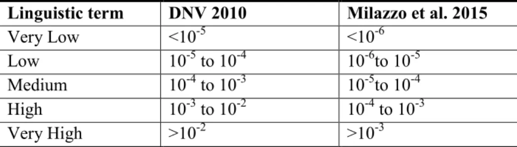
Table 2- 3: Failure Probability Scale of Assessment (DNV 2010) Category Annual Frequency Description
1 <10-5 So low frequency that event considered negligible.
2 10-5 to 10-4 Event rarely expected to occur.
3 10-4 to 10-3
Event individually not expected to happen, but when summarized over a large number of pipelines have the credibility to happen once a year.
4 10-3 to 10-2 Event individually may be expected to occur during the lifetime of the pipeline. (Typically 100-year) 5 >10-2 Event individually may be expected to occur more than once during the lifetime.
Inline inspection data was widely used by previous researchers to develop a model to estimate the POF (Caleyo et al. 2009, Sinha 2002, and Ahammed 1998, and Sinha and Pandey 2002). Caleyo et al. (2009) developed probability distribution functions of corrosion depth and rate of growth applying Monte Carlo simulation. Different curves were proposed for underground pipelines considering the properties of various soil types.
uncertainties of pipeline parameters. Both obtained data from Inline inspection tools to predict the failure probability of oil and gas pipelines under corrosion. These tools were used to gather data on the condition of oil and gas pipelines. The models required data on defects’ depth and length from inline inspection tools. Sinha and Pandey (2002) applied ANN to develop a model to predict the probability of failure of oil and gas pipelines. This model used the metal loss to forecast the burst pressure of such pipelines based on the model developed by Kiefner et al. (1973). The estimated pressure was used to forecast the remaining strength of the pipelines. Noor et al. (2011) proposed a probabilistic method to forecast the remaining strength of offshore pipelines obtaining data from inline inspection tools. This method was developed based on the assessment rules of DNV’s Recommended Practice for Corroded Pipelines (Veritas 2010) considering the standard deviation of inspection tools in determining the size of defects.
Qualitative researches on POF evaluation model applied expert opinion to develop a POF assessment model (Al-Khalil et al. 2005, Zeng and Ma 2009, Dawotola et al. 2009, Dey 2003, and Dey 2004). Al-Khalil et al. (2005), ranked a group of cross-country pipelines applying AHP. They classified risks of failure in seven groups: corrosion, mid wall defects, external interference, structural defects, operation problems, and loss of ground support. Then, experts scored the probability and cost of failure for each pipeline against the identified risk factors to calculate the overall expected cost of failure for each pipeline. These scores were later used to prioritize pipelines with respect to the budget. This Research tried to offer a “systematic risk-based approach” to prioritize a group of pipelines; although, it lacked the objectivity and did not develop a comprehensive model.
applied two sets of variables, general, and inspection and correlated them with six major types of failure titled: shape, seam, and structural failures, pipe alignment, and blockage. Then, it considered the consequences of failure, cost, performance, interruption, and safety, and finally offered a max-average method to maximize the effect of severe consequences in assessing the risk level. As the author described, this model did not develop any rating index to calculate the probability of failure. It only proposes an ordinal table of scales for different consequences; the absence of objectivity was apparent in this model.
Dey (2003) evaluated the risk of failure of various segments of a cross-country pipeline. The probability of failure of segments of a pipeline was assessed based on the judgment of experts comparing various sources of failure in each segment against the other sources. The calculated weights for each source of failure were considered as the likelihood of failure for each segment. These weights were then used to prioritize different segment to be inspected. Also, the inspection tool was selected based on the relative likelihood of failure of segments versus each other. Dey (2004) applied a similar method to calculate the probability of failure on oil and gas pipelines. Several experts judged the importance of different sources of pipeline failures applying AHP. The relative importance of the identified sources of failure was evaluated based on the calculated weights. Finally, the expert opinion was applied to rate the probability of failure of pipelines against each type of failure. This score multiplied by the calculated weights resulted in the calculation of failure probability.
Dawotola et al. (2009) proposed a model to calculate the failure probability of different causes of pipeline incidents. The model was designed with the combination of AHP and
Fault Tree Analysis (FTA). In fact, the model aimed to rank the causes responsible for pipeline failures based on the expert opinion. The model did not consider properties of the pipelines and only evaluated the relative importance of each failure cause.
Some of the previous studies used the artificial neural networks to develop a model on the probability of failure of pipes due to corrosion or third party activities. Bersani et al. (2010) proposed a model to predict the probability of failures with respect to different causes, applying Artificial Neural Networks. For each cause of failure, a set of factors was proposed as independent variables. Preliminary results were presented to predict the third party failures; however, results did not prove the importance of the proposed factors and neither the soundness of the model. Ren et al. (2012) applied back propagation neural networks in a model to predict the maximum corrosion rate of natural gas pipelines. Input variables included pipeline length, the difference of elevation between different sections, pipe inclination, and pressure. The model also considered the Reynolds number as an important factor in predicting the corrosion rate of various sections of gas pipelines. Menon (2005) defined the Reynolds number as an important factor in classifying the flow of natural gas pipelines. The study developed a function of average gas velocity, inside diameter of pipe, gas density and velocity as input parameters to compute the Reynolds number.
An extensive effort has been performed over the past years to model the reliability of the pipes subject to corrosion. Feng et al. (2011) developed a physical model for oil and gas pipelines. This research studied the effect of several factors on pipelines’ reliability. Data was obtained through “field measurement and physical and mechanical tests.” Sensitivity
thickness of the pipelines. Teixeira et al. (2008) developed a model to assess the reliability of pipelines with corrosion defects. The model computed the probability of pipelines’ failure based on the calculation of their burst pressure. It applied the numerical computations of reliability of the pipes. Sensitivity analysis proved the importance of corrosion depth and internal operational pressure on the burst failure of pipelines. The model was developed based on limited data from some field tests.
Forecasting the cause of failure for oil and gas pipes has been the subject of study for many researchers. Bertolini et al. (2006) developed a decision support system (DSS) to forecast the spillage class in the cross-country oil and gas pipelines. Classification and Regression technique was applied to develop a decision tree that was aimed at forecasting the cause of leakage in such pipelines. The objective of the research was to select the most appropriate inspection tool of oil and gas pipelines. Regression technique was applied to develop this model. Developed model was aimed to recognize pipelines with potential third party failures from those prone to the natural hazards failures. The model used variables such as pipe diameter, service type, location type, the age of failure, the environment, and the equipment used for detecting the leakage. Data was collected from Concawe (Davis et al. 2010) to forecast the cause of failure.
Senouci et al. (2013a) predicted possible failure sources for oil and gas pipelines applying
regression and ANN models. The models considered forecasting failure types besides corrosion, such as mechanical, third party, natural hazard, and operational failures. The models obtained historical data on the failures of pipelines in Europe that was prepared by Concawe (Davis et al. 2010). The accuracy of the model was acceptable; however, it applied only five variables for all failure types. These variables included the type of
product, pipe location, pipe age, land use, and pipe diameter. Except the age, variables remained constant over the life of a pipeline and consequently did not represent the changes that may happen in the environment and pipe itself. Also, as the author mentioned, the model applied a limited number of factors that can be developed to forecast the failure rate of other types. These limitations were mostly due to the model’s reliance on the Concawe database.
Most of the developed models were either subjective and were dependent on the expert judgment (Dey et al. 2004 and Dey 2003) or only addressed one source of failure of pipelines such as corrosion (Liao et al. 2012; Ren et al. 2012; Sinha and Pandey 2002; and Ahammed 1998). Consequently, they were not comprehensive. They also lacked the objectivity in estimating various sources of failures in oil and gas pipelines.
Several researchers tried to develop models to cover these limitations. They attempted to develop models that could predict other sources of failures besides corrosion. Senouci et al. (2013b) applied fuzzy logic technique to develop a model in order to predict the failure
type of oil and gas pipelines and compared the results with those of Senouci et al.
(2013a). The comparison results proved that the developed fuzzy-based model
outperformed the regression and ANN models with respect to the model validity. Despite the attempts made to predict the failure type of oil pipelines considering causes other than corrosion developed pipeline condition assessment models did not apply other factors besides corrosion. In other words, they mainly addressed factors that cause failures due to corrosion or third party damages only. In addition to that, the important issues of “interdependency” between different factors’ relations and “uncertainty” of factors’
(2014a) developed a model to evaluate the condition of oil and gas pipelines applying a
number of factors comprising corrosion. The model applied Analytic Network Process (ANP) and Monte Carlo simulation. Interdependency of factors was considered through ANP, and the suggested decisions took the uncertainty into consideration (using simulation). The implementation of the model on an existing offshore gas pipeline in Qatar was successful. The results of the model were compared with the actual pipeline condition.
The simulation model built by El-Abbasy et al. (2014a) was considered as a first phase to
evaluate or assess the condition of offshore oil and gas pipelines. El-Abbasy et al. (2014b)
developed the second phase of the model the objective of which was to predict the current and future condition of offshore oil and gas pipelines. The model was developed based on the historical inspection data that was collected in Qatar. The developed model used the regression analysis technique to predict the pipeline condition and when compared with the actual condition yielded an average validity percentage above 96%. El-Abbasy et al. (2014c) applied ANN technique to develop another model with the same
objective. The ANN model outperformed the regression model with respect to the validity results. These models applied several factors in predicting the condition of pipelines with considerably high accuracy. However, they could not develop a model to predict the sources of failures or their consequences. Also, the models designed in these studies were dependent on inline inspection data, which is expensive to gather frequently. They did not consider the specification of the location of pipes in developing the models. Shahriar et al. (2012) developed a comprehensive model to assess the risk of failure on oil and gas pipelines applying Bow-tie analysis. Bow-tie analysis is a new approach that
takes advantage of graphical techniques to analyze different scenarios of pipeline failures. This technique combines Fault Tree Analysis (FTA) with Event Tree Analysis (ETA). The model used the fault tree developed by Dawotola et al. (2009) and Yuhua and Datao (2005) with some modifications. Figures 2-2, 2-3 and 2-4 present the FT that was applied in this model. The Bow-tie diagram for the natural gas pipeline was centered over the gas release of the pipeline that was the top event for the fault tree. Sources of failure such as third party activities, corrosion, incorrect operation, unreasonable design, and geological hazards were the first level of expanding the causes of failure. In the lower levels, the variables that were in charge of different failure types were identified and considered as the basic events. Expert opinion was used to assess the fuzzy likelihood of basic risk events.
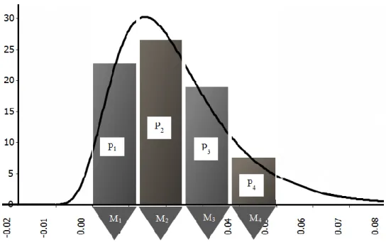
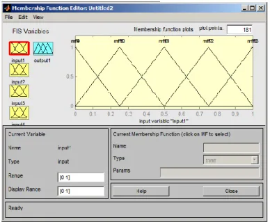
An 11-grade fuzzy scale was used to assess the probability of failure, which was developed by Sadiq et al. (2004). Triangular fuzzy membership functions were applied to develop the granular scale to evaluate the likelihood of failure. The scale translated the linguistic terms into fuzzy numbers evaluating the probability of failure from absolutely low to absolutely high level. The probability of the occurrence of final event was calculated by multiplying the probabilities attributed to the basic events. Finally, sensitivity analysis proved the importance of bad installation and construction defects. As mentioned before, the expert opinion was used to analyze the failure probability of gas pipelines. However, it was very hard for the experts to analyze the effect of 40 basic events on the failure probability of the final event (Shahriar et al. 2012). The limitations of the model can be minimized by applying the historical data in developing the model.
Some researchers tried to develop models to forecast the probability of failure as mentioned before (Shahriar et al. 2012; Dawotola et al. 2009; Yuhua & Datao 2005; Muhlbauer 2004; Kiefner 1997). In Tables 2-5, 2-6 and 2-7, the variables that were considered when developing the aforementioned models to estimate the probability of failure are summarized for each type of failure.
Table 2- 4: Summary of the variables affecting the probability of corrosion failures
Failure Types Sources Variables
External Corrosion Shahriar et al. 2012 Failure of CP Failure of Coating
Soil corrosion (High temperature, low resistance, high water ratio, high salt, bacteria, low pH, electrical interference) Dawotola et al. 2009 Failed CP Soil corrosion Failure of coating Yuhua & Datao
2005 Failure of CP Failure of Coating Soil Corrosion Anti-corrosion Muhlbauer 2004 Subsurface environment
soil corrosivity (resistivity, pH, moisture, carbonates)
Mechanical corrosion (stress level, stress cycling, temperature, coating, CP, pH)
CP effectiveness
Interference potential (DC & AC related, shielding potential)
Coating (type, age, visual inspection age, other inspection age)
Kiefner 1997
Pipe wall thickness CP efficiency Soil factor Experience factor Internal Corrosion Shahriar et al. 2012 Failure of inhibitor Failure of coating Debonding Dawotola et al. 2009 Failure of inhibitor Failure of coating Interfacial debonding Corrosive medium Yuhua & Datao
2005
Anti-corrosion Failure of inhibitor Failure of coating Bad clear pipe
Medium (with water or acid) Muhlbauer 2004
Flow characteristics Product corrosivity
Flow stream characteristics (solid and water related) Preventions
Table 2- 5: Summary of the variables affecting the probability of operational failures
Failure Types Sources Variables
Construction and Material Defects
Shahriar et al.
2012 The same as Yuhua & Datao 2005 Yuhua &
Datao 2005
Construction defect Material defect
Operation defect (bad installation, weld, groove Mechanical damage) Muhlbauer 2004 Inspection Materials Joining Backfill Handling Coating Kiefner 1997 MAOP
Hydrostatic test pressure Age factor
Seam factor Girth weld factor
Incorrect Operation
Shahriar et al.
2012 The same as Yuhua & Datao 2005 Yuhua &
Datao 2005
Quality of worker, SCADA, Equipment maintenance, Apparatus maintenance Muhlbauer 2004 Procedures SCADA Drug-testing Safety program Survey Training
Mechanical error preventers
Bad Design
Shahriar et al.
2012 The same as Yuhua & Datao 2005 Yuhua & Datao 2005 Unreasonable strength Unsuitable material Muhlbauer 2004
Safety factor (MOP, OP, material strength, th., external Loading, OD., strength of fitting, valves, components) Fatigue
Table 2- 6: Summary of the variables affecting the probability of external failures Failure
Types Sources Variables
Third Party
Shahriar et al. 2012
Parties ignore signage Implicit signage Sabotage Overload Yuhua & Datao
2005
Parties ignore signage Implicit signage Sabotage Overload
Muhlbauer 2004
Minimum depth of cover (soil cover, type of soil, pavement type, warning tape or mesh, water depth) Activity level (population density, stability of the area, one-call, other buried utilities, anchoring) Aboveground facilities (vulnerability, threats such as traffic)
One-call system (mandated, response by owner, well-known and user)
Public evacuation (methods such as door to door, mail, advertisement, frequency)
Right of way condition (signs, markers, overgrowth, undergrowth)
Patrol (Ground and air patrol frequency, Ground and air patrol effectiveness)
Natural Hazards Shahriar et al. 2012 Earthquake Flood Subsidence
[The same as Yuhua & Datao (2005)] Yuhua & Datao
2005
Earthquake Flood Subsidence
Muhlbauer 2004 Land movements (seismic shaking, fault movement subsidence, landslide, water bank erosion)
CP: Cathodic Protection; MAOP: Maximum allowable pressure; HTTP: Hydrostatic test pressure; OD. Pipe outside diameter, OP: Operating Pressure
2.3.5 Consequences of Failure
There has been an extensive effort during the past decades to model the consequences of the failure of oil and gas pipelines. Some of the guidelines provided a qualitative scale of assessment for this parameter of risk assessment from various points of view. DNV (2010) considered the consequences of failures of oil and gas pipeline with respect to safety (personal), environmental and economic hazards. Economic consequences accounted for the possible pipelines’ production delay, whereas the safety consequences were proposed to be measured with respect to the personnel. The cost of repairing damages to the pipeline was ignored in evaluating the economic consequences as it was deemed negligible. The proposed method was based on the experts’ judgment and hence was subjective. Table 2-8 presents the scores that were defined in different levels of safety consequences.
Table 2- 7: Safety consequences scale (Adapted from: DNV 2010) Category Description
1(low) No person(s) are injured.
2 (not used)
3(medium) Serious injury, one fatality (working accident)
4 (not used)
5(high) More than one fatality (gas cloud ignition)
DNV (2010) defined the environmental consequences as the effects of the product release with respect to the eco-system. As a result, the amount of the product spillage was used to rank the environmental consequences of a pipeline failure as shown in Table 2-9. Different levels of economic consequences and their attributed delay of production are shown in Table 2-10. The method developed in this guideline is a subjective method and
needs experts’ opinion. However, the experts are not known of the risks of oil and gas pipelines that are mostly underground or are laid offshore.
Table 2- 8: Environmental consequences scale (Adapted from: DNV 2010a)
Category Description
Amount of release 1(low) None, small or insignificant on the environment. Either due to
no release of internal medium or only insignificant release. ~ 0 2 Minor release of polluting media. The released media will
decompose or be neutralized rapidly. <1,000 tones 3(medium)
Moderate release of the polluting medium. The released media will use some time to decompose or neutralize, or can easily be removed.
<10,000 tones 4 Large release of the polluting medium which can be removed, or will after some time decompose or be neutralized. <100,000 tones 5(high) Large release of high polluting medium which cannot be
removed and will use long time to decompose or be neutralized. > 100,000 tones Table 2- 9: Economic consequences scale (Adapted from: DNV 2010a)
Category Description
Production delay/ Downtime 1(low) Insignificant effect on operation, small or insignificant cost of repair 0 days
2 Repair can be deferred until scheduled shutdown, some repair costs will occur. <1 month 3
(medium)
Failure causes extended unscheduled loss of facility or system and significant repair costs. Rectification requires unscheduled underwater operation with prequalified repair system before further production.
1-3 months
4
Failure causes indefinite shutdown and significant facility or system failure costs. Rectification requires unscheduled underwater operation without pre-qualified repair system before further production.
Or
Failures resulting in shorter periods of shutdown of major parts of (or all of) the hydrocarbon production for the field.
3-12 months
5(high)
Total loss of pipeline and possible also loss of other structural parts of the platform. Large cost of repair including long time of shut down of production.
Or Failures resulting in shutdown of the total hydrocarbon production for a longer period.
Some researchers tried to develop numerical models to estimate the consequences of the pipelines’ failure. Resterpo et al. (2009) developed logistic regression models to predict the monetary consequences of pipeline failures. The models obtained data from the office of pipeline safety (OPS) a section of the US Department of Transportation (DOT). Data on the incidents of the hazardous liquid pipelines from 2002-2005 was obtained to develop this model. First, the probability of occurrence of non-zero consequences was assessed through logistic regression models. The models were trained embedding data on several parameters from the database. The parameters included the system part involved in the accident, location of the pipeline (offshore versus onshore), occurrence in a high consequence area (HCA versus non-HCA), as well as the binary factors representing the occurrence of ignition, explosion and/or product loss. For non-zero consequence incidents, other models were developed. The inputs of these models included characteristics of the incidents such as the occurrence of ignition and/or explosion, the amount of the product loss, the location specifications (i.e., offshore versus onshore, and HCA versus non-HCA), the system part involved, and the cause of the accident. These models could be used to analyze different scenarios of accidents on such pipelines. However, there were some limitations in their application to predict the consequence of failures. First, the amount of the product loss and the part of the system involved in the incident is very hard to predict and is not known before the happening of an accident. Besides, the models were not validated, and their accuracy in the prediction of monetary consequences was not tested.
the failures of transmission and distribution pipelines respectively. Similar to Resterpo et al. (2009) this study developed a two-step model. In the first step, the probability of the occurrence of a non-zero cost consequence was evaluated through logistic regression models. These models included binary variables on the incident characteristics of pipelines failure. In the second step, the magnitude of a cost consequence was measured applying least square regression models. These models used variables presenting the causes of incidents and incident types. Results of the models were the scenarios of pipelines’ failure. One of the scenarios was the failure of an onshore transmission pipeline as a result of internal corrosion in a non-HCA with rupture. This scenario was assumed not to be involved with an ignition or explosion. The computed cost of failure was predicted to be in the interval of 17,093 to 281,815 the average of which was calculated as 71,093 US$. The analyzed scenarios did not consider the characteristics of the pipeline such as diameter, wall thickness or age. As a result, the models developed in this study cannot be applied to assess the consequences of failure risk of a specific pipeline.
Event Tree (ET) was used by some of the researchers to model the consequence of failures of oil and gas pipes. Brito et al. (2009) developed an event tree to analyze the accidental failures of natural gas pipelines. The main factors that were considered in developing this event tree were failure mode (rupture versus puncture), delay in the possible ignition, as well as the “degree of space confinement” of released gas. Consequences of the product release were identified as: detonation, Jet fire, Confined Vapor Cloud Explosion (CVCE), Flash Fire and gas dispersion. An additive function of human, environmental, and financial consequences was considered to calculate the
consequence probabilities. Each pipeline was divided into sections covering tens of meters. The probability of consequences for each section was computed obtaining the experts’ opinion through probabilistic judgments. However, it had been very hard for the experts to estimate the probability distribution function of the consequences’ happening. As a result, the average pipeline failure rate was used as the failure probability that was calculated based on the EGIG reports (2009). This average value was used as the basic failure probability in gas pipelines that was equal to 0.00041/km. per year. Some adjusting factors including land use and soil, third party activities, distance from residential areas were used. The experts estimated the value of the adjusting factors in different sections of the pipeline. Consequently, the sections were ranked according to their risk of failure. Although, the model benefited from the historical data, it was subjective and depended on the experts’ opinion. Besides, the experts needed to be highly experienced as the model needed detailed data on the estimation of the adjusting factors. As mentioned before, Shahriar et al. (2012) developed a “Bow-tie” analysis model that considered the post-failure events of gas pipelines to estimate the consequences of failure. Figure 2-5 depicts the event tree developed by this model. This model adapted the ET developed by Sklavounos and Rigas (2006). The main factors that were considered in developing the ET were mentioned as the delay in the ignition of the released gas due to the pipe failure and the degree of space confinement. The events after a gas release were identified as Detonation, Fireball, Confined Vapor Cloud (CVC) explosion, Flash Fire, and material loss. The probability of the occurrence of each post-failure event was assessed by multiplying the probability of gas release by the probability of happening of
resulted in analyzing the probability of happening of each scenario of failure. Then the triple bottom line sustainability criteria were used to evaluate the social, environmental, and economic consequences of failures. Social consequences included the assessment of casualty, society response and evacuation requirement. Environmental consequences required the evaluation of consequences with respect to the air, endangered habitats, vegetation, soil, and water. Finally, economic evaluation of the consequences included the effects of failure on supply interruption, repair, material loss, and property and third party damages. The granular fuzzy scale was applied to assess the consequences of each failure scenario by experts’ opinion (Shahriar et al. 2012). Applying expert elicitation decreased the objectivity of the model and made it difficult for the experts to judge the probability of occurrence of each scenario and estimating several factors to estimate the consequences of a pipeline failure.