DOI:10.1142/S0218539312400025
A MULTI-OBJECTIVE APPROACH TO OPTIMIZE A PERIODIC MAINTENANCE POLICY
ANTONELLA CERTA∗,MARIO ENEA†,GIACOMO GALANTE‡ and TONI LUPO§
Dipartimento di Ingegneria Chimica Gestionale,Informatica,Meccanica Universit`a degli Studi di Palermo
90128 Palermo,Italy ∗[email protected] †[email protected] ‡[email protected] §[email protected] Received 25 July 2012 Revised 15 September 2012 Accepted 14 November 2012 Published 3 January 2013
The present paper proposes a multi-objective approach to find out an optimal periodic maintenance policy for a repairable and stochastically deteriorating multi-component system over a finite time horizon. The tackled problem concerns the determination of the system elements to replace at each scheduled and periodical system inspection by ensuring the simultaneous minimization of both the expected total maintenance cost and the expected global system unavailability time. It is assumed that in the case of system elements failure they are instantaneously detected and repaired by means of minimal repair actions in order to rapidly restore the system. A nonlinear integer math-ematical programming model is developed to solve the treated multi-objective problem, whereas the Pareto optimal frontier is described by the Lexicographic Goal Program-ming and theε-constraint methods. To explain the whole procedure, a case study is solved and the related considerations are given.
Keywords: Periodic maintenance; multi-component system; nonhomogeneous Poisson process; multi-objective optimization.
1. Introduction
The majority of preventive maintenance problems considered in literature for multi-component systems1 concerns both the scheduling of the system inspections and the determination of the system elements to be maintained at each inspection. Such problems have been extensively studied in literature and several surveys have been developed.2,3 A particular kind of preventive maintenance policy for multi-component systems is the periodic one. In such a maintenance policy, each system
element can be replaced at fixed and periodic time intervals disregarding its failure history and repaired when a failure occurs.4The periodic maintenance policy rep-resents for its easy implementation, the most used maintenance policy, especially in large and complex multi-component systems. In fact, complex production systems such as power plants, gas turbines plants, petroleum refineries, etc., in order to reduce the failure probability and to satisfy the production and/or technological constraints, are generally subjected to periodically scheduled inspections during life cycle to verify functioning conditions with reference to the system safety, reliability and performance levels. During the scheduled inspections the potential and hid-den failures are detected and fixed and, in addition, also preventive maintenance can be performed on no-defective selected elements. The periodic maintenance was introduced and investigated for the first time by Barlow and Hunter5 and, from that moment on, many maintenance models and optimization approaches have been developed assuming one or more objective functions and some operative constraints. The most treated objective in this kind of maintenance policy is the minimiza-tion of the total maintenance cost. For example, Briset al.6developed a single objec-tive optimization model, considering the system elements periodically inspected and maintained, aiming to find out the optimal maintenance policy for each element by minimizing the cost function and respecting the availability constraint. In order to solve the problem, the authors propose a genetic algorithm, whose structure includes the inspection time and the time length between two maintenance interventions for each element.
Wang and Pham7investigated maintenance cost and availability, optimal main-tenance policies of the series system with n constituting components under the general assumption that each component is subject to correlated failure and repair, imperfect repair, shut-off rule, and arbitrary distributions of times to failure and repair. In particular, two classes of maintenance cost models are proposed and sys-tem maintenance cost rates are modeled.
Caldeira Duarteet al.8proposed a mathematical programming model for a series system, with component characterized by a Weibull hazard function, to calculate the optimum frequency to perform preventive maintenance actions for each component. The goal is the minimization of the maintenance cost so that the total downtime, in a certain period of time, does not exceed a predetermined value. The authors show that the maintenance interval of each component depends on two factors: the failure rate and the repair and maintenance times of each component. Also Certa et al.9 formulate a constrained mono-objective mathematical model to solve the problem of determining both the optimal number of periodic inspections within a finite time frame and the system elements to replace at each scheduled inspection. The maintenance policy has to ensure a very high reliability level with the minimum total maintenance costs. The latter include costs directly related to the maintained elements, the system downtime and inspection costs.
Taghipouret al.10developed a model to find out the optimal periodic inspection intervals over a finite time horizon considering a system composed of components
subjected to soft and hard independent failures. Hard failures are instantaneously detected and fixed while soft failures can be detected and fixed only at the sched-uled inspections. The model takes into account as objective to optimize the expected total cost arising from soft and hard failures incurred over the optimization cycle and a recursive procedure is adopted to solve it. The researches previously described, as the present paper, concern developing maintenance models related to finite time intervals and in the matter of this aspect Nakagawa and Mizutani11offer an esting summary in which different policies of maintenance for a finite time inter-val are described. In particular, the authors propose modified replacement policies which convert three usual models of periodic replacement with minimal repair, block replacement and simple replacement to replacement ones for a finite time span. Furthermore, they propose an imperfect preventive maintenance model where the failure rate decreases by the means of the preventive maintenance actions. Finally, the authors consider the periodic and sequential inspection policies in which a unit is checked at successive times for a finite time.
Taghipour and Banjevic12 developed a model aiming to determine the optimal periodicity of the inspection intervals of a reparable system subjected to hidden fail-ures over finite and infinite optimization time intervals. A failed system component may be replaced or minimally repaired with a probability dependent on the compo-nents age. Recursive procedures are developed to calculate probabilities of failures, the expected number of minimal repairs and the expected downtime of the system. The considered objective function is the minimization of the expected total cost.
Grigoriev and Van De Klundert13 treat a scheduling problem, with relation to a periodic maintenance problem, by offering a note on the integrality gap of an integer linear program formulation previously introduced by Grigorievet al.14
Considering production systems, a suitable parameter for evaluating the mainte-nance policy effectiveness is the stationary availability, also defined as the expected time percentage in which the system is functioning. Therefore, also the station-ary availability maximization represents another objective to be reached in mainte-nance optimization processes. Vaurio15studied the average unavailability of standby units under several sets of assumptions concerning the renewal efficiency of tests and repairs. In particular, the author develops a general formalism for selecting economically optimal test and maintenance intervals, with and without a risk con-straint. Basic cost, equations and several optimal intervals solutions have been obtained for different testing/failure categories by proposing different maintenance policies. Unavailability equations are developed by the same author under the age-replacement policy. Testing (or inspection) is performed at fixed intervals. Tests discover failures but they do not have any effect on the subsequent reliability char-acteristics of a unit: it is “as good as old but unfailed” after a successful test. The unit is periodically renewed after a fixed number of test intervals or whenever a failure occurs. The model includes maintenance times and cost contributions due to inspections, repairs, maintenance and loss of production. Several necessary and sufficient conditions and solution techniques are developed for optimizing tests and
maintenance intervals, with and without availability constraints. Cassady et al.16 tackled the problem to single out the set of components on which to operate at peri-odic scheduled breaks, in order to maximize the system availability and respecting the maintenance costs constraint. The maintenance activities must be completed within an allotted time. The problem is formulated by a mathematical model and solved for two simple systems. Tsaiet al.17 developed an algorithm to find out an optimal maintenance policy for a multi-component system. The authors consider a preventive maintenance policy that takes simultaneously into account three actions: the mechanical service, aiming at alleviating the strength degradation, the repair activity, addressed to partially restore a degraded component and the replacement activity, settled to recover a component to its original condition. For each com-ponent the preventive maintenance intervals are investigated on the basis of the system availability maximization and the minimum interval value is chosen for pro-gramming the periodic maintenance policy.
In the light of the previous considerations, in this paper the maintenance cost and the system unavailability time are considered as objective functions. In fact, system unavailability and maintenance cost could take a different importance depending on the different scenarios in which the decision maker operates. The two objective functions are contrasting to each other and therefore, it is not possible to find a single solution corresponding to the best result for all of the two considered objectives but a set of nondominated trade-off solutions. A solution is defined as nondominated if it is better than the others with relation to at least one objective. The concept of nondominated solutions implies that in a multi-objective optimiza-tion problem an “optimal” soluoptimiza-tion does not exist, but optimality is related to trade-offs between different objectives. Clearly, an efficient optimization procedure should generate a number of different nondominated solutions among which the decision maker should select the most attractive one. According to this framework, the optimization of a multi-objective problem means exploring the solution space in order to determine the nondominated solutions, which lies on a boundary region named Pareto-Frontier.
In literature, maintenance problems formulated by multi-objective models have been basically solved by two different approaches. The first approach requires a pref-erence vector to construct a composite function so converting the multi-objective problem into a single-objective one. An example of the application of such a method-ology in the maintenance field is proposed by Lapa et al.,18 which consider relia-bility and cost as objectives. A composite function is formulated and the single objective optimization problem is solved by a genetic algorithm. The difficulty in normalizing the objective functions and in quantifying the weights is well known. In any case, if a priori knowledge of a reliable preference vector is available, such an approach would be adequate, otherwise the input information is employed with-out any knowledge of the possible consequence. A more recent approach consists in splitting the solution procedure into two phases. The first step consists in selecting
the set of nondominated trade-off solutions (Pareto optimal solutions) within the whole space of feasible ones respecting the constraints. In the second step, the Pareto frontier solutions are evaluated and compared in order to select the best one. The hardest aspect of this approach is to obtain the Pareto optimal frontier. Certaet al.(2011) applied this methodology on a multi-objective maintenance con-test related to an interval between two consecutive inspections. In particular, the goal is addressed to the determination of the set of elements on which maintenance actions must be executed so that the system operates with a required reliability until the next scheduled inspection, minimizing both the maintenance total cost and the total maintenance time. In order to solve the previous constrained multi-objective optimization problem, an algorithm able to rapidly solve the problem is proposed and its effectiveness is shown by an application to a complex series–parallel system.
More recently, heuristic approaches to the problem, like evolutionary algorithms, have been developed. Nevertheless they often imply high computational time and they do not ensure the determination of the overall Pareto optimal frontier. Hilber et al.19 applied the multi-objective approach to a real system of power delivery. In particular, the aim is the determination of the optimal trade-off between pre-ventive and corrective maintenance in order to maximize customer satisfaction and to minimize maintenance cost. Some solutions belonging to the Pareto frontier are obtained by applying two different methods: the first one is a simple heuristic opti-mization approach, whereas the second one is based on an evolutionary algorithm. The authors highlight that the first approach is prone to fall into a local opti-mum while the second does not present this disadvantage but it requires a higher computational time. Chang and Yang20 developed a multi-objective optimization model in order to carry out a proper preventive maintenance scheduling for a power supply substation that is able to provide an effective trade-off between reliability and maintenance cost. The authors state that the traditional methods applied to the multi-objective maintenance scheduling problems imply high computational efforts. They propose a multi-objective genetic algorithm and the minimum cut set method. Martorell et al.21 classify the GA approaches for the multi-objective problems into two categories. The first one, the Single Objective Genetic Algo-rithms (SOGA), transform the multi-objective problems into a mono-objective one by means ofa prioridefinition of a preference vector. In this way, the SOGA provide a single solution at each algorithm run, belonging to a nondominated frontier. The other, the Multi-Objective Genetic Algorithms (MOGA), simultaneously find a set of nondominated solutions. Algorithms belonging to this category are, for exam-ple, the Niched Pareto Genetic Algorithm (NPGA),22the NSGA-II,23the strength Pareto evolutionary algorithm (SPEA).24 The two categories are compared with reference to their capacity to describe the Pareto frontier. The authors state that the first category allows focusing on a particular region of the solution space while the second one better describes the Pareto frontier. In both cases, an extremely
high number of generations are necessary to obtain a set of Pareto solutions. An overview of multi-objective GAs proposed in literature for reliability optimization problems can be found in Konaket al.25
The simplest and probably the most widely used approach to describe the Pareto frontier is the weighted sum method.26 The greatest difficulty in applying this method consists in setting suitable weight vectors to obtain optimal nondominated solutions. Moreover, this method is able to describe only the convex region of the frontier. The ε-constraint method27 constitutes another classical methodology. It overcomes the limitation of the previous one but its use, when more than two objectives are taken into account, is laborious because the found solutions largely depend on the chosenεvector and a bad choice could not lead to feasible solutions. Such method consists in reformulating the multi-objective optimization problem considering only one of its objectives and restricting the remaining ones within user-chosen valuesεi; in such way single-objective optimization problem typical solution methods can be used to obtain a single Pareto frontier solution corresponding to the chosen values of theεi.
The latter approach is herein used in order to describe the Pareto frontier of the considered multi-objective optimization problem.
The present paper is organized as follows: the multi-objective optimization prob-lem is presented in Sec. 2 and mathematically formulated in Sec. 3; in Sec. 4 the adopted resolution approach is given and in Sec. 5 a case study is solved and the related results are commented; finally, the conclusions close the work.
2. The Multi-Objective Optimization Problem
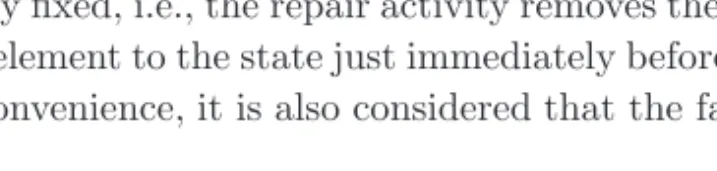
As mentioned before, it is herein considered a reparable and stochastically deterio-rating multi-component system consisting of several components arranged in series that, in their turn, can be constituted by a single element or by parallel-series ele-ments. Because of its own functional features and operative conditions, the system can be stopped for inspection and replacement activities just at some fixed and periodical instants j = 1,2, . . . ,(P−1) being tp the time between two successive inspections andT = (P−1)·tpthe considered optimization time frame (see Fig.1). During the system operative time, the failed elements are instantaneously detected and minimally fixed, i.e., the repair activity removes the failure at minimal effort and returns the element to the state just immediately before the failure. More-over, for the sake of convenience, it is also considered that the failures of elements,
j=1 j=2 j=3 … j=(P-1) j=P
tp tp tp
T
belonging to components composed of parallel-series elements, are instantaneously detected and minimally repaired while the system is in the functioning condition.
As said before, the aim of the developed approach is to single out the elements set to replace at each scheduled inspection so that the minimization of both the total maintenance cost and the global unavailability time of the system over the cycle length T is ensured. The number of the considered planned inspections in the optimization procedure represents a trade-off between the goal of extending the temporal horizon in order to obtain solutions closer to the long term optimal ones and the one of reducing computational time that rapidly grows up at increasing the number of intervals. Finally, at the end of the optimization periodj =P, it may assume that a major system overhaul will be performed and a new cycle will start again, then a new optimization procedure should be applied.
3. Mathematical Problem Formulation The following nomenclature is hereafter used:
i= 1,2, . . . , N index representing a generic element;
b= 1,2, . . . , Bi index representing a generic branch of a component i arranged in parallel;
eb index representing the elements arranged in series in the branchb;
j= 1,2, . . . ,(P−1) index representing a generic inspection;
k= 0,1, . . . ,(P−1) index representing the last inspection in which replace-ment of the generic elereplace-ment has been performed. k takes value equal to zero if the last replacement has been performed before the beginning of the optimiza-tion temporal horizon;
xi,j binary variable takes 1 if the element i is replaced at the inspectionj;
ri,j,k reliability of the elementi calculated at the inspection
j until the inspectionj+ 1, when the last replacement has been performed at the inspectionk;
Ccm unit time cost of maintenance crew for minimal repairs;
Ccp unit time cost of maintenance crew for replacement
activities;
CDTp unit time cost of system downtime for inspection; CDTm unit time cost of system downtime for failure;
cri cost of the spare part for replacement of the elementi;
cmi cost of the spare part for minimal repair of the elementi;
Tj time duration of inspectionj;
tri replacement time of the elementi;
The proposed approach can be formulated by a nonlinear integer mathematical programming model with the following two objective functions:
minC, (1)
minU, (2)
where C and U are the functions of the expected values of the total maintenance cost and the system unavailability time, respectively, over the cycle length T. The function of the expected total maintenance cost can be expressed as:
C=
P−1
j=1
(Cj+Cm,j), (3)
where Cj is the cost arising from the replacement activities performed during the inspectionj, whileCm,jis the cost of the minimal repairs performed in the operative time between the inspectionjand the next onej+1. The costCjincludes the spare parts costs, those for the allocated maintenance crews and also the downtime costs:
Cj =
N
i=1
(cri+Ccp·tri)·xi,j+CDT p·Tj. (4)
Since the maintenance crews can operate in parallel during the system inspections, it is assumed that the system downtime cost is directly proportional to the longest maintenance time among those of the elements replaced during each inspection. Such a condition is ensured by the following constraint:
Tj≥tri·xi,j, ∀j, ∀i. (5)
The cost of the minimal repairsCm,j includes the costs of spare parts for minimal repairs, the maintenance crew costs, and only for the failure modes that imply the stop of the system, the downtime costs. In particular, if the failure concerns a branch of a component arranged in parallel, the system is still able to continue working during the minimal repair activity and therefore that failure mode does not imply system downtime cost. Instead, if the failure occurs on a component composed of a single element, also the downtime cost has to be considered since it implies that the system stops. Thus, the expected total cost Cm,i,j, for minimal repairs of a componentibelonging to the setZ of the system components arranged in parallel, are given by the following equations:
Cm,i,j= Bi b=1 eb k=1 cm,k·mk,j+Tm,i,j·Ccm, ∀i∈Z and ∀k∈i, (6) where cm,k is the cost of the spare part for minimal repair of the element k, and
between the inspection j and the next onej + 1, whose formulation operative is given by the following relationship:
Tm,i,j= Bi b=1 eb k=1 tm,k·mk,j, ∀i∈Z and ∀k∈i, (7) with tm,k and mk,j the minimal repair time and the number of failures of the elementk, respectively.
In the same way, the expected total cost for minimal repairs of the component
ibelonging to the setS of the components composed of a single element are given by Eq. (8):
Cm,i,j = [cm,i+ (CDT m+Ccm)·tm,i]·mi,j, ∀i∈S. (8) Therefore, the minimal repair costs functionCm,j is given by:
Cm,j =
i∈Z
Cm,i,j+
i∈S
Cm,i,j. (9)
In a similar way, the function of the expected system unavailability time U over the cycle lengthT can be formulated. Such function can be expressed as the rela-tionship (10): U = P−1 j=1 Tj+ i∈S tm,i·mi,j . (10)
Finally, under the hypothesis of minimal repair, the expected number of system element failures follows a nonhomogeneous Poisson Process (NHPP) with a power law intensity function. In such a case, the expected number of failure of the element
imi(t), within the time period [0, t], is given by the following equation:
mi(t) = t 0 λi (t)·dt= t 0 fi(t) Ri(t)·dt=−lnRi(t), (11) being λi(t), fi(t) and Ri(t) the failure rate, the probability density function and the reliability of the considered element, respectively.
3.1. Reliability calculation
The reliability of the elementi, at a generic scheduled inspection j until the next scheduled inspectionj+ 1, can be expressed as:
Ri,j =ri,j,j·xi,j+
j−1
k=0
(ri,j,k·zi,j,k)·(1−xi,j), ∀k
0 ≤k < j. (12) Wheneverxi,j is equal to 1, i.e., the elementi is replaced at the inspection j, the related reliability value is given by ri,j,j. On the contrary, when xi,j is equal to zero, the replacement of the elementiis performed at the inspectionk, withk < j and k = 0 if the element i has not been replaced until the inspection j. When
the last replacement occurs at the inspectionk, the reliability value of the element
i is given by ri,j,k that represents the conditional reliability whose calculation is successively explained. In Eq. (12) the term zijk is a binary dummy variable that makes mutually exclusive the two conditions previously described, i.e., the two terms of the expression (12) related to the instant in which the element has been replaced, that is at stopj or at a previous system stop.
To ensure such condition, the following conditions have to be satisfied:
• whenxijtakes value equal to 1,zijkis equal to zero for anyk;
• whenxij is equal to zero,zijkis equal to 1 only for the inspectionkin which the last replacement of the elementihas been performed.
To satisfy the aforementioned conditions the constraint (13) has to be fulfilled:
zi,j,k=xi,k·
j
n=k+1
(1−xi,n), ∀k/0≤k < j. (13)
The previously introduced reliability functionri,j,j is expressed by:
ri,j,j =Rij(tj+1−tj) =Ri,j(tp), (14) where, as said before, tp denotes the system operative time between the two con-secutive scheduled inspectionsj andj+ 1.
According to the theory of the probability, the reliability function ri,j,k (Eq. (14)), is given by the following equations:
ri,j,k = Ri,j(tj+1−tk) Ri,j(tj−tk) = Ri,j((j+ 1−k)·tp) Ri,j((j−k)·tp) ∀j, ∀k|k= 0, (15) ri,j,k = Ri,j(tj+1) Ri,j(tj) = Ri,j(j·tp+tstart,i)
Ri,j((j−1)·tp+tstart,i)∀j, and withk= 0, (16) wheretstart,iis the age of the elementiat the first inspectionj = 1.
By considering the Weibull probability distribution, with the shape parameter
βι > 1 and the scale parameter ηi > 0 of the element i, the relations (14)–(16) become: ri,j,j = exp − tp ηi βi ∀j, (17) ri,j,k= exp −(j+ 1−k)·tp ηi βi exp − (j−k)·tp ηi βi ∀j, ∀k|k= 0, (18)
ri,j,k= exp − j·tp+tstart,i ηi βi exp − (j−1)·tp+tstart,i ηi βi ∀j, and withk= 0. (19) 4. Resolution Approach
In order to individuate the extreme Pareto-optimal solutions, the Lexicographic Goal Programming (LGP) method is initially used. This method separately con-siders the two objective functions, thereby reducing a multi-objective problem into a mono-objective one. For example, these sequential steps determine the extreme solution of minimum cost:
• minimizingC as a single objective problem obtainingCmin;
• minimizingU considering the previous value ofCas a further constraint obtaining
Umax.
The procedure is analogously applied by changing the objectives hierarchy to find the other two boundsCmax and Umin of the extreme solution of minimum system unavailability time. Once the extreme points of the Pareto frontier are determined, theε-constraint method is used to individuate other Pareto solutions. As suggested by Haimes et al.,27 the problem can be modified by keeping one of the objectives and restricting the others within specified values. Hence, Pareto-optimal solutions can be found by using different sets of “εi” that must be chosen within the minimum and maximum values of the objective functions previously found by using the LGP method. The choice of a particular set of values forεirestricts the possible location of the solution to a desired region of the Pareto-optimal frontier.
In our case, having just two objective functions, it is sufficient to minimize one of the two objective functions and restricting the remaining one within user-specified values ε. In particular, in the first step, minimizing C and considering the value
Umax as a constraint, a new solution can be found. Successively, the procedure is carried out by imposing that the U function has to take a value less to that one corresponding to the solution previously found and by minimizing theC function. The procedure is repeated until the extreme solution is obtained. In such a way, theε-constraint method ensures the exploration of the entire Pareto frontier is also in the presence of nonconvex region in the Pareto frontier.
5. Case Study
In order to show how the developed multi-objective optimization approach works, a case study has been solved. In particular, it is considered a multi-component system that is periodically stopped for inspections to perform replacement actions that cannot be executed during the system operative time. The system is composed, from a reliability point of view, by seven series components. The first one is constituted
by elements in a parallel-series disposition with two branches, each one constituted by two elements; the second component is a simple parallel component with three branches, while the other components are constituted by a single element. Totally, the system comprises 12 elements.
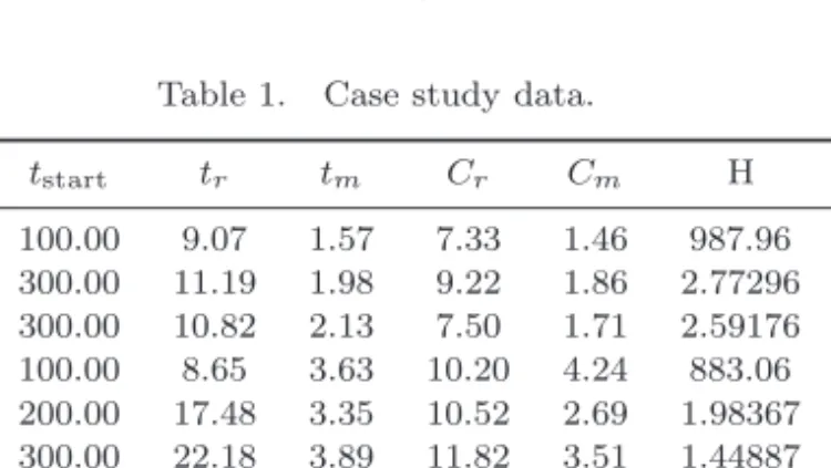
As said before, for each element the reliability function is modeled by a Weibull distribution whose parametersηandβare reported in Table 1. The table also shows the cost data, expressed in monetary units (M.U.), the time data in time units (T.U.) and the age of the system elements tstart,i at the beginning of the opti-mization horizon. All the data have been randomly generated within opportune ranges.
The model has been solved by the commercial software Lingo, assuming the following parameters values:
tp= 800 T.U.; T = 2400 T.U.; CDTp= 10 M.U.; CDTm= 500 M.U.;
Ccp= 1 M.U.; Ccm= 2 M.U.
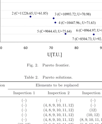
The optimization procedure is started by applying the LGP method, the solution numbers 1 and 7 have been found. They constitute the extremes of the Pareto frontier. Successively, the ε-constraint method is applied in order to describe the whole Pareto frontier (Fig. 2). In fact, as explained in Sec. 4, the ε-constraint method is able to explore the entire Pareto frontier and since in this case there are only two objectives to optimize, the method assures the complete description of the Pareto frontier. Thus, even if the range limited by the extreme solutions for the two objectives is wide, the entire optimal solutions space, that is the Pareto frontier, is constituted by only seven solutions.
It is meaningful to highlight that the obtained Pareto frontier shown in Fig. 2 is not convex and, one more time, theε-constraint method shows its capability in indi-viduating solutions in nonconvex regions of the Pareto frontier. Table 2 indicates, for each optimal solution, the corresponding replacement plan.
Table 1. Case study data.
Element tstart tr tm Cr Cm H B 1 100.00 9.07 1.57 7.33 1.46 987.96 1.92 2 300.00 11.19 1.98 9.22 1.86 2.77296 1.38 3 300.00 10.82 2.13 7.50 1.71 2.59176 1.23 4 100.00 8.65 3.63 10.20 4.24 883.06 1.95 5 200.00 17.48 3.35 10.52 2.69 1.98367 1.38 6 300.00 22.18 3.89 11.82 3.51 1.44887 1.41 7 100.00 12.17 2.06 7.79 2.01 813.92 1.33 8 300.00 18.75 3.63 10.96 3.06 1.21847 1.81 9 100.00 15.91 2.97 9.05 2.50 3.22668 1.33 10 100.00 11.58 2.21 10.66 1.83 1.35061 1.68 11 200.00 17.63 3.26 11.48 2.71 1.95564 1.20 12 300.00 9.83 1.72 9.35 1.52 1.53156 1.67
Fig. 2. Pareto frontier.
Table 2. Pareto solutions. Solution Elements to be replaced
Inspection 1 Inspection 2 Inspection 3
1 (–) (–) (–) 2 (–) (4,8,9,10,11,12) (–) 3 (–) (4,8,9,10,11,12) (12) 4 (–) (4,8,9,10,11,12) (10,12) 5 (–) (4,8,9,10,11,12) (8,9,10,11,12) 6 (10,12) (4,8,9,10,11,12) (8,9,10,11,12) 7 (8,9,10,11,12) (8,9,10,11,12) (8,9,10,11,12) 6. Conclusion
The presented optimization model wants to offer a contribution to the scientific literature on periodic maintenance field in the case in which the periodical inspec-tions do not regard the system single component but the whole system. Because of its own functional features and operative contests, the system can be stopped for inspection and replacement activities just at some fixed and periodical instants. Therefore, the time between two consecutive inspections is not considered here as decisional variable. However, if technological and/or operative conditions allow, the developed model is able to quantify possible benefits due to a different periodicity value. The aim of the developed approach is to single out the elements set to replace at each scheduled inspection so that the minimization of both the total maintenance cost and the global unavailability time of the system is ensured.
The optimal periodic maintenance policy is individuated within a finite opti-mization horizon that goes over the next scheduled inspection, so to obtain the solu-tions closer to the long-term optimal ones. The number of considered inspecsolu-tions
will be a compromise between the goals of extending the temporal horizon and that of reducing computational time that rapidly grows up at increasing the number of intervals.
Another meaningful aspect with respect to the literature and closed to the real operative contests is the multi-objective approach to the problem and in particular the research of nondominated solutions. In fact, the knowledge of the Pareto frontier supplies to the decision-maker further information about the problem, first of all costs and system unavailability ranges in which the solution will fall down. The choice of a low cost or low time solution will depend on the specific contest in which the decision-maker will be called to operate. Whenever an operational readiness is required to the system, then a low system unavailability solution will be chosen, vice versa a low cost solution will be selected whenever it is possible to increase the system breakdown. If budget availability and/or system unavailability time constraints are present, the sub-set of optimal feasible solutions on which to restrict the selection is immediately individuated. Moreover, the frontier analysis could directly address the decision-maker to discard some solutions (as the solutions 6 and 3 of the previews case study) that imply small cost reductions but a meaningful unavailability time increments with respect to other solutions (as the solutions 5 and 2).
Finally, if the Pareto optimal frontier includes lots of solutions, the decision-maker could be supported by a decision multi-criteria method as the Analytic Hierarchy Process (AHP)28 or the ELimination Et Choix TRaduisant la REalit`e (ELECTRE)29 in order to select the solution that represents the best compromise among the considered objectives.
References
1. D. Cho and M. Parlar, A survey of maintenance models for multi-unit systems,Eur. J. Oper. Res.51(1991) 1–23.
2. C. Valdez-Flores and M. R. Feldman, A survey of preventive maintenance models for stochastically deteriorating single-unit systems,Naval Res. Logist.36(1989) 419–446. 3. R. Dekker, F. A. Schouten and R. Wildeman, A review of multi-component main-tenance models with economic dependence, Math. Meth. Oper. Res. 45(3) (1997) 411–435.
4. H. Wang, A survey of maintenance policies of deteriorating systems, Eur. J. Oper. Res.139(2002) 469–489.
5. R. Barlow and L. Hunter, Optimum preventive maintenance policies, Oper. Res.8 (1960) 90–100.
6. R. Bris, E. Chˆatelet and F. Yalaoui, New method to minimize the preventive mainte-nance cost of series-parallel systems,Reliab. Engrg. Syst. Safety82(2003) 247–255. 7. H. Wang and H. Pham, Availability and maintenance of series systems subject to
imperfect repair and correlated failure and repair, Eur. J. Oper. Res. 174 (2006) 1706–1722.
8. J. A. Caldeira Duarte, J. C. Taborda, J. T. Craveiro and T. P. Trigo, Optimization of the preventive maintenance plan of a series components system,Int. J. Pressure
Vessels Piping 83(2006) 244–248.
9. A. Certa, G. Galante, T. Lupo, A. Passannanti and G. Passannanti, A model for a periodic preventive maintenance policy for a series parallel system, inProc. 19th Int.
Conf. Flexible Automation and Intelligent Manufacturing, Middlesborough, UK, 6–8
July 2009, pp. 1026–1033.
10. S. Taghipour, D. Banjevic and A. K. S. Jardine, Periodic inspection optimization model for a complex repairable system, Reliab. Engrg. Syst. Safety 95(2010) 944– 952.
11. T. Nakagawa and S. Mizutani, A summary of maintenance policies for a finite interval, Reliab. Engrg. Syst. Safety94(2009) 89–96.
12. S. Taghipour and D. Banjevic, Periodic inspection optimization models for a reparable system subjected to hidden failure,IEEE Trans. Reliab.60(1) (2011) 275–285. 13. A. Grigoriev and J. Van De Klundert, A note on the integrality gap of an ILP
formu-lation for the periodic maintenance problem,Oper. Res. Lett.39(2011) 252–254. 14. A. Grigoriev, J. Van De Klundert and F. Spieksma, Modelling and solving the periodic
maintenance problem,Eur. J. Oper. Res.172(2006) 783–797.
15. J. K. Vaurio, Availability and cost functions for periodically inspected preventively maintained units,Reliab. Engrg. Syst. Safety63(1999) 133–140.
16. C. R. Cassady, E. A. Pohl and W. P. Murdock Jr., Selective maintenance modelling for industrial systems,J. Quality Maintenance Engrg.7(2) (2001) 104–117.
17. Y. T. Tsai, K. S. Wang and L. C. Tsai, A study of availability — Centered preventive maintenance for multi-component systems,Reliab. Engrg. Syst. Safety84(2004) 261– 270.
18. C. M. F. Lapa, C. M. N. A. Pereira and M. Paes de Barros, A model for preven-tive maintenance planning by genetic algorithms based in cost and reliability,Reliab.
Engrg. Syst. Safety 91(2006) 233–240.
19. O. Hilber, V. Miranda, M. Matos and L. Bertling, Multi-objective optimization applied to maintenance policy for electrical networks,IEEE Trans. Power Syst.22(4) (2007) 1675.
20. C. S. Chang and F. Yang, Inspection frequencies for substation condition-based main-tenance,Naval Platform Technology Seminar, Singapore, 16–17 May 2007.
21. S. Martorell, A. S´anchez, S. Carlos and V. E. Serradell, Alternatives and challenges in optimizing industrial safety using genetic algorithms, Reliab. Engrg. Syst. Safety
86(2004) 25–38.
22. R. Rajagopalan and C. R. Cassady, An improved selective maintenance solution approach,J. Quality Maintenance Engrg.12(2006) 172–185.
23. K. Deb, S. Agrawal, A. Pratap and T. Meyarivan, A fast and elitist multi-objective genetic algorithm: NSGA-II,IEEE Trans. Evol. Comput.6(2002) 182–197.
24. E. Zitzler, Evolutionary algorithms for multi-objective optimization: Methods and applications, Ph.D. thesis, Swiss Federal Institute of Technology, Zurich (1999). 25. A. Konak, D. W. Coit and A. E. Smith, Multi-objective optimization using genetic
algorithms: A tutorial,Reliab. Engrg. Syst. Safety 91(2006) 992–1007.
26. K. Deb, Multi-Objective Optimization Using Evolutionary Algorithms (John Wiley and Sons, New York, 2001).
27. Y. Y. Haimes, L. S. Lasdon and D. A. Wismer, On a bicriterion formulation of the problems of integrated system identification and system optimisation, IEEE Trans. Syst., Man Cybern. 1(3) (1971) 296–297.
28. T. L. Saaty,Fundamentals of Decision Making and Priority Theory with the Analytic
Hierarchy Process (RWS Publication, Pittsburg, PA, 2000).
29. B. Roy, The Outranking Approach and the Foundations of ELECTRE Methods in Reading in Multiple Criteria Decision Aid, ed. C. A. Bana e Costa (Springer-Verlag, Berlin, 1990), pp. 155–183.
30. A. Certa, G. Galante, T. Lupo and G. Passannanti, Determination of Pareto frontier in multi-objective maintenance optimization,Reliab. Engrg. Syst. Safety 96(7) (2011) 861–867.
About the Authors
Antonella Certa received Master degree in Management Engineering in 2004 and the Ph.D. degree in the Economic Analysis, Technology Innovation and Manage-ment of the DevelopManage-ment Policy Studies Program in 2008 from the University of Palermo. She is currently a researcher and she is Professor of Industrial Plants at the Department of Production Engineering of the University of Palermo (Division of Agrigento). Dr. Certa’s research interests are mainly focused on project manage-ment, multi-criteria analysis and maintenance optimization models.
Mario Enea is Full Professor at the University of Palermo in Project Management, Industrial Plant Management. His present research fields include themes regarding the production management, the project management, optimal layout problems. He has been scientific manager in several projects of applied research sponsored by the Italian Government and the public and private companies particularly in the field of the project management.
Giacomo M. Galante is Full Professor of Industrial Plants at the University of Palermo, Italy. His present research fields are mainly focused on industrial plant layout optimization, reliability and maintenance policies, risk analysis and project management. He has been scientific manager in several projects of applied research sponsored by the Italian Government and the public and private companies partic-ularly in the field of the maintenance optimization and risk analysis.
Lupo Toni received Master degree in mechanical engineering from the University of Palermo, Italy in 1996, and the Ph.D. degree in Industrial Engineering from the same university, in 2003. He is currently a researcher at the Department of Production Engineering of the University of Palermo and he is Professor of Quality Industrial Management. His research interests are in reliability optimization and statistical method of reliability modeling. Dr. Lupo is a member of the Italian Association of Mechanical Technology.