Modelling water demand and availability scenarios for current and future land use and climate in the Sava River Basin

(1)

Ad De Roo, Bernard Bisselink, Hylke Beck, Jeroen Bernhard, Peter Burek, Arnaud Reynaud, Marco Pastori, Carlo Lavalle, Chris Jacobs-Crisioni, Claudia Baranzelli, Zuzanna Zajac, Alessandro Dosio

Addressing

the

water-food-energy-ecosystem nexus

Modelling water demand and

availability scenarios for current and

future land use and climate in the

Sava River Basin

(2)

This publication is a Technical report by the Joint Research Centre (JRC), the European Commission’s science and knowledge service. It aims to provide evidence-based scientific support to the European policy-making process. The scientific output expressed does not imply a policy position of the European Commission. Neither the European Commission nor any person acting on behalf of the Commission is responsible for the use which might be made of this publication.

Contact information Name: Ad de Roo

Address: EC Joint Research Centre, Via E. Fermi 2749, TP 121, 21027 Ispra (Va), Italy E-mail: [email protected] Tel.: 0039-0332-786240 JRC Science Hub https://ec.europa.eu/jrc JRC99886 EUR 27701 EN

Print ISBN 978-92-79-54585-6 ISSN 1018-5593 doi:10.2788/789075 LB-NA-27701-EN-C PDF ISBN 978-92-79-54586-3 ISSN 1831-9424 doi:10.2788/52758 LB-NA-27701-EN-N

Luxembourg: Publications Office of the European Union, 2016

Reproduction is authorised provided the source is acknowledged.

How to cite: De Roo A, Bisselink B, Beck H, Bernhard J, Burek P, Reynaud A, Pastori M, Lavalle C, Jacobs C, Baranzelli C, Zajac Z, Dosio A. (2016), Modelling water demand and availability scenarios for current and future land use and climate in the Sava River Basin; Luxembourg (Luxembourg): Publications Office of the European Union; EUR 27701 EN; doi:10.2788/52758

All images © European Union 2016, except:

Frontpage: Strbacki buk-Una (Strbacki rapids in Una river at near Bihac, Bosnia Herzegovina) Author: Miroslav Jeremic, 2015. Source: International Sava River Basin Commission

(3)

Acknowledgements

This research and publication is a result of a close collaboration with the International Sava River Basin Commission. Specifically, the staff of the ISRBC secretariat is thanked for the fruitful contacts: Mr Dejan Komatina, Mr Samo Groselj and Mr Dragan Zeljko. Several members of the Sava commission working group on river basin management have made useful comments and suggestions for further work. These suggestions, additional data and feedback is used in the forthcoming Danube Nexus report, which will include the Sava as well.

Furthermore, a good collaboration on this research was established with UNECE (Ms Annukka Lipponen) and the Royal Institute of Technology (KTH, Stockholm Sweden) (Prof. Mark Howells and colleagues).

The EURO-CORDEX community (http://euro-cordex.net/ ) is gratefully acknowledged for the supply of the climate projections.

Last but not least it should be mentioned that this work is a collaborative effort within JRC with several groups participating. Some of them are included as co-author, but several others have directly or indirectly contributed as well to this report.

(6)

Abstract

The impact of various combinations of land use change, climate change and policy measures on the water-energy-food-environment nexus in the Sava river basin has been evaluated through 170 simulations with the LISFLOOD water resources model for 30-year periods. The LISFLOOD model was first calibrated and validated for the Sava basin against weather and river discharge observations, which were partially obtained from the International Sava River Basin Commission. The goodness-of-fit score obtained for the most downstream station for the calibration period was 0.91, suggesting that the model performance was excellent overall. Also, it was found that the model performance was relatively consistent amongst sub-catchments of the Sava river basin.

For the Sava river basin, we found in this study that more intense irrigated agriculture does have the potential to increase crop yields considerably, but available water resources are not sufficient to realise this. Also, if irrigation would be increased drastically, other sectors would be negatively influenced, such as the energy sector (reduced cooling water availability, potentially less water at times produce hydropower), navigation (more frequent and lower low-flows), and the environment (breaches of environmental or minimum flow conditions).

With respect to most of the water resources indicators, the projected land use changes until 2050 balance each other out, and the net effect is only marginal. Land use projections for Slovenia until 2050 show a substantial increase of forested area at the expense of arable land and semi-natural vegetation. Urban land use is expected to increase by roughly 22% as compared to present day; industrial land use is expected to increase by roughly 27%. For Croatia, forest areas are expected to increase substantially between 2010 and 2050 until 50% of the country’s land surface is forested. Areas of arable land and semi-natural vegetation are expected to decrease substantially. Industrial and urban land uses are expected to increase by respectively 22% and 1%. Effects on water resources would be more significant with increased irrigation to increase the crop yield of e.g maize. This would lead to an increase in water demand from 2216 Mm3/year to 3337 Mm3/year. Overall water demand in the Sava basin would further increase to around 6000 Mm3/year if we combine both increased irrigation and climate projections until 2100. The average simulated maize yield could increase from 5.7 tons/ha at present conditions to 9.9 tons/ha in case of increased and optimum irrigation. These substantial increases in irrigation, which would lead to substantial crop yield increases as well, would lead to water scarcity in parts of the Sava basin. Also, there just is not sufficient water to irrigate all areas which are water-limited for crop growth. Existing irrigation plans and irrigating the areas which were previously equipped for irrigation (according to FAO) seems more feasible from a water resources perspective. Flood peaks are projected to remain unchanged as a consequence of projected land use changes until 2050 for the Sava basin. However, with climate change projections we do simulate an overall increase in the flood peaks with 13% for the 2011-2040 period and a 23% increase for the 2071-2100 period.

River low-flows decrease moderately for the 2011-2040 scenarios. For the end of the century 2071-2100, lowflow values are projected to moderately increase as compared to the control 1981-2010 climate. Excessive irrigation would result in a severe decrease of the lowflow discharges with 50-60%. As for ecological flows, similar observations can be made.

(7)

Water availability for energy production - hydropower and cooling water for thermal and nuclear power stations – is projected to decrease by an average of 3.3% for 2030 under RCP4.5, whereas RCP8.5 would result in a 1.3% increase. End of the century simulations yield a 17.6% higher Q50 for RCP4.5 and 23.1% higher for RCP8.5. Excessive irrigation could affect the water availability for power production, especially for cooling thermal power stations. Hydropower reservoirs could be turned into multi-functional reservoirs, also serving downstream irrigation needs and flood control, and thus serve multiple purposes.

Soil water stress conditions, which would potentially reduce agricultural crop yields, are especially affecting the lower parts of Bosnia-Herzegovina, Croatia and Serbia under current climate. Climate impact simulations show an increase of soil water stress of 9% for 2030. For the end of the century, RCP4.5 shows a 1% increase, whereas RCP8.5 shows a 7% increase in soil water stress. This might indicate stronger needs for irrigation in the future to maintain current crop yields.

Our climate impact simulations show a moderate decrease of groundwater resources for Slovenia and the higher parts of Croatia and Bosnia Herzegovina until 2030. For the end of the century runs we observe increases in groundwater resources. Increased irrigation practices would seriously reduce groundwater resources again. Also, if relatively more groundwater is used for irrigation replacing surface water, groundwater resources decrease as well.

Feedback of Sava River Basin Commission experts has been taken into account and the suggested improvements will be used in the forthcoming Danube Water Nexus report.

(8)

1. Introduction and aim of the research

1.1 Policy context and background

The Joint Research Centre (JRC) provides scientific support to the European Union Strategy for the Danube Region (EUSDR) in two ways. Firstly, it addresses the scientific needs related to the implementation of the EUSDR and thereby helps decision-makers and other stakeholders to identify the policy needs and actions needed for the implementation of the Strategy. Secondly, it contributes to the reinforcement of ties and cooperation amongst the scientific community of the Danube Region.

The JRC Scientific Support to the Danube Strategy initiative is sub-divided into different flagship clusters and activities. They aim to address the scientific challenges faced by the Danube Region from an integrated and cross-cutting perspective, taking into account the interdependencies between various policy priorities.

Four thematic clusters focus on the key resources of the Danube Region, namely water, land and soils, air, and bioenergy. The four thematic clusters are complemented by three horizontal activities: The Danube Reference Data and Service Infrastructure (DRDSI), Smart Specialisation, and the Danube Innovation Partnership (DIP).

The Danube Water Nexus (DWN) flagship cluster covers various water-related issues such as water availability, water quality, water-related risks and the preservation and restoration of ecosystems and biodiversity. It also aims to analyse the interdependencies of between different water-intensive economic sectors such as agriculture and energy. Within the Danube Water Nexus a case study is carried out on the Water-Energy-Food-Ecology Nexus within the Sava River Basin. This study has been executed in close collaboration with the UNECE and its partner the Royal Institute of Technology (KTH, Stockholm, Sweden) and the International Sava River Basin Commission (ISRBC).

The Danube Water Nexus further aims to support the International Commission for the Protection of the Danube River (ICPDR) and the International Sava River Basin Commission (ISRBC). Furthermore, the research carried out here aims to provide insight and advice to establish Programs of Measures within the Water Framework Directive (WFD), and the Flood Risk Management Plans of the Floods Directive (FD).

1.2 Objectives

The aim of the JRC Water Nexus study is to examine various water futures in the Sava River Basin.

Climate change and land use changes driven by political, demographical and economic factors will have consequences for the balance between water availability and water demand of various sectors. Further changes in the agriculture and energy sector will also be of influence.

Situations may arise, when agricultural or industrial activities may face water shortages, or that insufficient water is available for hydropower operations or for cooling purposes of other power plants. This balance between availability and demand is studied here, and consequences of potential measures are investigated.

(9)

• Provide an overview of current water resources and pressures in the Sava River Basin, under current climate and current land use practices

• Evaluate future changes in water demand, water resources and pressures under projected land use changes until 2050

• Evaluate the additional effect of climate change projections for the Sava River Basin on water resources and pressures

• Evaluate the effects of various policy measures on water resources and water availability for the various economic sectors, including the environment, agriculture, energy production and navigation.

• Evaluate the water availability for hydropower and thermal power stations, as well as changes of the water availability due to climate change, land use change, and policy measures.

1.3 The Sava River Basin

The Sava River is the third longest and the largest by discharge tributary of the Danube River. The length of the Sava River from its main source in western Slovenian mountains to its mouth to Danube in Belgrade is about 944 km (source: ISRBC). The Sava river runs through four countries (Slovenia, Croatia, Bosnia and Herzegovina, and Serbia) (Figure 1).

The Sava river basin has a surface area of 97,713 km2 and covers considerable parts of Slovenia, Croatia, Bosnia and Herzegovina, Serbia, Montenegro and a small part of the Albanian territory (Table 1).

Figure 1 Sava River Basin Overview (Source: International Sava River Basin Commission - ISRBC)

(10)

With an average discharge of about 1564 m3/s, the Sava River is the most important Danube tributary with respect to discharge, contributing with almost 25% to the Danube's total discharge at the confluence of the Sava and Danube river in Belgrade (Serbia).

Table 1 Country statistics in the Sava river basin (sources: ISRBC and JRC LISFLOOD model estimates, based on Eurostat current reported water demands)

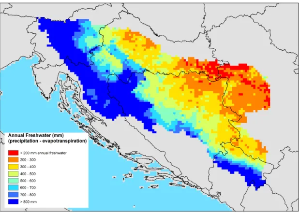
Figure 2 Annual net runoff (precipitation minus evapotranspiration) for the Sava basin, reference period 1990-2013.

(11)

2. Modelling methods

This chapter describes the various models that are used in this study. The main water resources calculations are done with the LISFLOOD model. Land use projections are made with the LUISA model, and fed into LISFLOOD with 5-year intervals. The EPIC model was used for the maize crop yield simulations and scenarios.

2.1 The LISFLOOD model

LISFLOOD is a GIS-based spatially-distributed hydrological rainfall-runoff model developed at the JRC. It includes a one-dimensional hydrodynamic channel routing model (De Roo et al., 2000; Van der Knijff et al., 2010; Burek et al., 2013). LISFLOOD is currently used at the JRC for simulating water resources in Europe and Africa. Driven by meteorological forcing data (precipitation, temperature, potential evapotranspiration, and evaporation rates for open water and bare soil surfaces), LISFLOOD calculates a complete water balance at a daily time step (for this study) and every grid-cell.

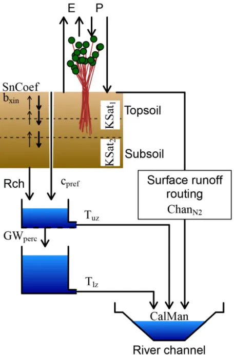
Figure 3 The grid-based LISFLOOD model.

2.1.1 Model design and theory

Processes simulated for each grid cell include snowmelt, soil freezing, surface runoff, infiltration into the soil, preferential flow, redistribution of soil moisture within the soil profile, drainage of water to the groundwater system, groundwater storage, and groundwater base flow. Runoff produced for every grid cell is routed through the river network using a kinematic wave approach.

(12)

The model has also options to simulate lakes, reservoirs, and retention polders, which are relevant for low-flow analysis (as they tend to increase low flows) as well as for simulating flood protection during high flows. In the current setting for Europe, 1680 lakes and reservoirs are included. For the global model setup, in total 9300 lakes and reservoirs are included.

A detailed description of the meteorological, soils, vegetation and land use data used for this study can be found in chapter 3 of this report.

(13)

2.1.2 Applications of LISFLOOD

Although this model has been developed with the aim of carrying out operational flood forecasting at the pan-European scale, recent applications demonstrate that it is well suited for assessing droughts and the effects of land-use change and climate change on hydrology (Feyen et al., 2007; Dankers and Feyen, 2009), as well as general water resources (Burek et al, 2012; De Roo et al., 2012). Recently, the model has been applied in Africa (Thiemig et al., 2013) and for global applications (Beck et al., 2015; De Roo et al., 2015).

With a grid size of 5 x 5 km (Europe) and 0.1 x 0.1 degree (global scale), LISFLOOD is developed for simulating medium and large river basins. Satisfactory results can be obtained in basins of a few hundred km2 up to the size of the entire Danube basin. A limiting factor is the availability of good, accurate and homogenous input data for the area of interest, for example soil data, accurate meteorological forcing data or measured discharge data for model calibration. Human influences (e.g. dams, reservoirs, polders, irrigation) also are difficult to quantify, and available data are often scarce. This is an especially important factor for low-flow simulations.

2.1.3 Sub-grid processing

The current pan-European setup of LISFLOOD, which is also used here for the Sava River Basin, uses a 5-km grid and spatially variable input parameters and variables. While the model operates on the relative coarse scale of 5km resolution, subgrid information on land use (100m), soils (1km) and elevation (100m) is used for several sub-grid processes.

This is done to account properly for land-use dynamics, for which also some conceptual changes have been made to render LISFLOOD more use sensitive. Combining land-use classes and modelling aggregated classes separately is known as the concept of hydrological response units (HRU). This concept is used in models such as SWAT (Arnold and Fohrer, 2005) and PREVAH (Viviroli et al., 2009) and is now implemented in LISFLOOD on the sub-grid level.

LISFLOOD uses the fractions of landuse within a 5x5km pixel. The model distinguishes for each grid the fraction of forested areas, built up areas, water surface, irrigated land, paddy rice land, and other land use. These fraction maps have been derived from the 100m resolution LUISA land use model output maps. The spatial distribution and frequency of each class is defined as a percentage of the entire (in this case 5 x 5 km) grid. Like this, details of the 100x100m level will remain for a large part. For example changes in urban coverage from 2% to 3% within a 5x5km area are still taken into account.

To address the sub-grid variability in land use, we model the within-grid variability by running the soil modules separately for fractions of land use. Several model processes are simulated seperately:

100m elevation information is used to establish several altitude zones within the 5km grid, important for snow accumulation and snowmelt modelling. Also 100m elevation is used to correct surface temperatures.

(14)

2.1.4 Water demand, abstraction and consumption

Water demand for livestock, manufacturing industry, energy production (cooling water needs), and public sector water use are input grids for LISFLOOD and in line with the land use data.

Crop irrigation and paddy-rice irrigation needs are simulated dynamically. Crop irrigation is simulated depending on soil moisture and evapotranspiration deficits, thus dynamically responding to changes in weather and climate, during the model runs. For the actual water abstraction, the efficiency of the used irrigation type (sprinkler or drip irrigation) is taken into account, as well as conveyance efficiency.

Paddy rice irrigation is simulated by initial saturation at the start of the growing season, and then assuming a 5cm water ponding in the rice fields, until 3 weeks before harvesting. The water is either drained into the soil or evaporates.

Actual water abstraction is calculated while checking if the demand can actually be met. Specifically, the model takes into account if the water is abstracted from groundwater, lakes or reservoirs, or is available from non-conventional sources, such as desalination plants. The remaining water is abstracted – if a available – from the river surface water. A – user defined - minimum flow threshold is built in in LISFLOOD to prevent discharge going below a certain predefined level, to mimick ecological flow constraints.

Net water consumptions from the various sectors are calculated taking into account for example the type of cooling facility, or using fixed consumption coefficients for e.g. public water use and livestock water use. LISFLOOD takes into account return flow to the river or soil.

For the moment, LISFLOOD contains a fixed water allocation scheme, by which irrigation gets the last priority. User-definable water allocation schemes are being built in at the moment.

2.1.5 Model output and indicators used for this study

The LISFLOOD model can basically output any internal variable used, such as river discharge, soil moisture, snow cover or evapotranspiration. In addition, specific water resource indicators have been developed as well as output options. Output can be time series (hydrographs), summary maps or stacked maps over the complete time period. Below, the main variables and indicators used in this study are listed:

State variable outputs

• Discharge (m3/s) in rivers as maps • Hydrographs for specific points

• Water volumes in lakes and reservoirs (m3)

• Soil moisture content in any of the three soil layers (m/m) as maps • Soil moisture at specific location as timeseries

• Groundwater level in lower groundwater zone (LZ) (mm)

Indicator outputs:

(15)

• Water Exploitation Index • Water Dependency Index

• Sectorial water demands, abstractions, and net consumption • Root Water Stress Indicator

• Environmental flow indicator

• Evaporation deficit or Climatic Water Deficit

2.1.6 Discharge statistical indicators

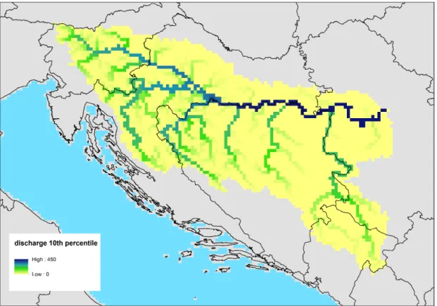
Figure 5 The discharge 10th percentile, simulated with LISFLOOD using observed meteorological data 1990-2013 and present land use

From the simulated daily river discharges at each location and for all the multiple year runs, the following percentiles are calculated:

• Q001: discharge value, for which 0.1% of duration Q is lower, and during 99.9% Q is higher (once in 1000 days low flow)

• Q01: discharge value, for which 1% of duration Q is lower, and during 99% Q is higher (once in 100 days low flow)

• Q05: discharge value, for which 5% of duration Q is lower, and during 95% Q is higher (once in 20 days low flow, ~ 18 days per year low flow)

• Q10: discharge value, for which 10% of duration Q is lower, and during 90% Q is higher • Q25: 25% quartile, for which 25% of duration Q is lower

• Q50: median discharge value

(16)

• Q95: discharge value, for which 95% of duration Q is lower, and during 5% Q is higher • Q99: discharge value, for which 99% of duration Q is lower, and during 1% Q is higher (once

in 100 days high flow)

• Q999: discharge value, for which 99.9% of duration Q is lower, and during 0.1% Q is higher (once in 1000 days high flow)

In addition, also return period discharges can be calculated. To calculate those return periods, annual flood peaks from the simulated discharge series were fit to a Gumbel distribution. We have evaluated the HQ05, HQ10, HQ20, HQ50 and HQ100 return period discharge.

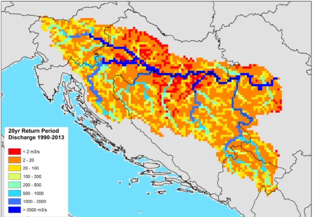
Figure 6 The 20-year return period discharge in the Sava basin, based on simulations with observed weather 1990-2013.

(17)

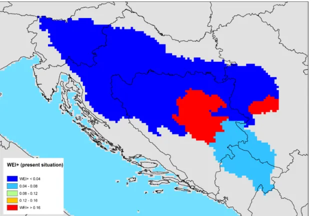
2.1.7 The Water Exploitation Index (WEI and WEI+)

The Water Exploitation Index (WEI) (withdrawal ratio) in a country is defined as the mean annual total abstraction of fresh water divided by the long-term average freshwater resources (EEA indicator fact sheet). It describes how the total water abstraction puts pressure on water resources. Thus it identifies those countries having high abstraction in relation to their resources and therefore are prone to suffer problems of water stress. The term average freshwater resource is derived from the long-term average precipitation minus the long-long-term average evapotranspiration plus the long-term average inflow from neighbouring countries. Values

WEI = Local Water Abstraction / (Local Renewable Freshwater + Upstream inflow)

The related Water Exploitation Index Plus (WEI+) (consumption ratio), is the total consumption divided by the long term freshwater resources of a country. This index highlights those regions with a higher consumptive use of water.

WEI+ = Local Water Consumption / (Local Renewable Freshwater + Upstream inflow)

Figure 7 The Water Exploitation Index (WEI+) estimated for the Sava for current conditions

(18)

2.1.8 The Water Dependency Index (WDI)

The Water Dependency Index (WDI) (De Roo et al 2015) of a country or a sub-riverbasin in a country is defined as the Local Water Demand that cannot be met by the Local Renewable Water Resources, as a fraction of Upstream Inflowing Water from cross-border river basins, thus:

Water Dependency = (Local Water Demand – Local Renewable Freshwater) / Upstream inflow

Water Dependency Index (WDI) values between 0 and 1 indicate that a region is depending on upstream inflow for a part of their local water needs. Higher values indicate stronger dependencies. WDI values above 1 indicate unsustainable situations, where additional upstream freshwater is also not sufficient to meet local water needs, and likely fossile groundwater or desalination is used to meet the remaining demand. Negative WDI values mean that the amount of locally renewable freshwater is higher than local water demand, and thus that regions or countries are self-sufficient.

Figure 8 Water Dependency Index for the Sava River Basin sub-regions, estimated using the LISFLOOD model. Only Serbia has a marginal water dependency.

(19)

2.1.9 Sectorial water abstraction and consumption

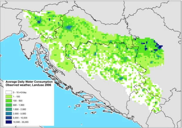
Water demands, abstractions, and consumption are summed up at local and/or regional level and per month and are available as indicator. Amounts are available for irrigation, livestock, energy, industry, and public sector water usage. LISFLOOD distinguishes between abstractions, return flow and net consumption.

Figure 9 Average Daily Water Consumption (m3 per 25km2 grid), for current climate and landuse.

(20)

2.1.10 The Root Water Stress index (RWS)

The Root Water Stress indicator shows the reduction of crop and/or vegetation transpiration due to limited water availability, following the standard FAO method. When the soil is wet, the water is relatively free to move and is easily taken up by the plant roots. In dry soils, the water is strongly bound by capillary and absorptive forces to the soil matrix, and is less easily extracted by the crop.

For soil water limiting conditions RWS lies between 0 and 1. Where there is no soil water stress, RWS equals 1. Both the daily RWS value and the number of days RWS<1 are optional LISFLOOD model output.

Figure 10 Example of LISFLOOD water stress output: the average number of days per year with water stress, resulting in limited transpiration, resulting in possible yield decreases.

(21)

2.1.11 Environmental flow indicator

LISFLOOD has an option to flag individual days and locations where a pre-defined discharge amount is not met, and then counts the total number of days over a defined period that discharge values are below this threshold.

For the moment, pending a better scientific and agreed definition of environmental flow in Europe, the 10% percentile of discharge is taken, calculated over the entire year, so ignoring - for now - seasonal effects or requirements etc.

At present we implement witihin the LISFLOOD model an option where abstraction can be limited if e-flow is to be respected, as well as a user-definable water allocation schemes.

Figure 11 Changes in the number of days per year that the Environmental Flow threshold is not met; difference between baseline 2006 scenario and land use 2050 with additional irrigation; note: the current land use change data only cover Slovenia and Croatia(EU28)

(22)

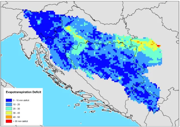
2.1.12 The evaporation deficit or climatic water deficit

The term climatic water deficit defined by Stephenson (1998) is quantified as the amount of water by which potential evapotranspiration (PET) exceeds actual evapotranspiration (AET). This term effectively integrates the combined effects of solar radiation, evapotranspiration, and air temperature given available soil moisture. Climatic water deficit can be thought of as the amount of additional water that would have evaporated or transpired had it been present in the soils given the temperature forcing. This calculation is an estimate of drought stress on soils and plants, and gives an indication of the climatic pressure on water resources, independent from human influences in the river basin.

The climatic water deficit can also be thought of as a surrogate for water demand based on irrigation needs, and changes in climatic water deficit effectively quantify the supplemental amount of water needed to maintain current vegetation cover, whether natural vegetation or agricultural crops.

Within the LISFLOOD model, the climatic water deficit is indeed used as an estimate for irrigation water needs as well.

Figure 12 Monthly average climatic water deficit (mm), estimated by LISFLOOD using 1990-2013 observed weather data.

(23)

2.2 The LISFLOOD model calibration procedure

LISFLOOD was calibrated to improve the response behavior of the model. For the calibration we used as objective function the Kling-Gupta Efficiency (KGE; Kling et al., 2012) computed between simulated and observe daily Q. We used the KGE, rather than the more widely used Nash and Sutcliffe (1970) Efficiency (NSE), because the latter is generally considered to be a weak metric of model performance (e.g., Criss and Winston, 2008). To evaluate the temporal transferability of the calibrated parameter sets, for each station the record of simultaneous forcing and observed Q data was split into a calibration and a validation period. If the record of simultaneous forcing and observed Q data was >10 years long, the second half was used for calibration and the first half for validation. If the record of simultaneous forcing and observed Q data was 5 to 10 years long, the last 5 years were used for calibration and the remainder for validation. If the record of simultaneous forcing and observed Q data was <5 years long, the station was discarded. In total 38 catchments were found to be suitable for calibration.

Evolutionary algorithms have been widely used for the calibration of hydrologic models (Wang, 1997; Maier et al., 2014). The (µ+λ) evolutionary algorithm was used to calibrate LISFLOOD against daily observed Q for the calibration period. The algorithm was implemented using the Distributed Evolutionary Algorithms in Python (DEAP) toolkit (Fortin et al., 2012). The population size (µ) was set to 32 and the recombination pool size (λ) to 64. Crossover and mutation probabilities were set to 0.9 and 0.1, respectively. For each generation, λ offspring were produced from the population. Offspring were evaluated, after which the population of the next generation was selected from both offspring and population. The number of generations was limited to 13, as this was found to be sufficient to achieve convergence in most cases. This resulted in 832 model runs and objective-function evaluations per catchment. The calibration of all 38 catchments lasted about 7 days on a workstation equipped with two Intel Xeon E5-2640 CPUs (total 16 cores and 32 threads).

2.3 The LUISA land use model

The future land use projections used in this study are modelled using the JRC platform for `Land-Use-based Integrated Sustainability Assessment’ (LUISA). Several scenarios have been modelled using that platform; for this study the results of the 2014 Reference scenario have been provided. For an overview of the Reference Scenario we refer to (Baranzelli, Jacobs-crisioni, et al., 2014). For a complete description of the LUISA modelling platform and its underlying mechanics we refer to (Batista e Silva et al., 2013; Lavalle et al., 2011).

The LUISA platform is developed to satisfy the EC’s growing need for an instrument for the ex-ante evaluation of its policies from a holistic perspective; thus, by taking into account the economic, social and environmental effects of those policies. The LUISA platform consists of dynamically interlinked models that are tasked with the computation of regional future land demand, accessibility levels, population distribution, land-use patterns and sustainability-related indicators. Next to a wide range of indicators, key outputs of the LUISA platform are fine resolution maps (100m x 100m grid cells) of accessibility, population densities and land-use patterns for each of the model’s time steps covering all 28 EU member states. In this section the land demand and land-use pattern aspects of the model will be briefly described, after which some of the results relevant for this report will be shown.

All results in the LUISA platform are governed by estimates of regional future land demand that are the direct or indirect results of various sectoral models. Those expected regional demands are fed into the LUISA platform with in the case of expected land

(24)

demand a short bandwidth of acceptable deviations from the input model. These land demands form fixed constraints for the area of land that the population and land-use models in LUISA may assign while running. Relevant regional inputs are Eurostat for population projections (EUROPOP 2011 scenario); GEM-E3 for economic projections; the CAPRI model for projections of agricultural land demand (PRIMESCOR scenario); and UNFCC for projections of changes in forested areas. The latter are based on trends of afforestation/deforestation that are obtained from national counts of forest area as declared to the UNFCC. In some cases additional data are used to obtain land demands from the specialised model outputs. For instance, GEM-E3 delivers estimates of future GDP. Those estimates are translated into expected demand for industrial areas by exploiting data on historical industrial land-use intensities. The mechanisms to obtain land-use demands from various specialised models are described in (Baranzelli, Castillo, et al., 2014)(Baranzelli, Jacobs-crisioni, et al., 2014).

As noted before the input population numbers and land demands are constraints for the LUISA modules that manage the spatial distribution of people and land-use patterns. Because in particular land-use patterns are relevant for the subject of this report, we will focus on the modelling of those land-use patterns here. For a description of the population allocation module we refer to (Batista e Silva et al., 2013). The land-use allocation module distributes discrete land-use classes by simulating competition between the modelled land-uses. Its core was initially based on the Land Use Scanner (Hilferink and Rietveld, 1999)(Koomen et al., 2011), CLUE and Dyna-CLUE (Verburg and Overmars, 2009; Verburg et al., 2002) land-use models (Verburg and Overmars, 2009; Verburg et al., 2002), but has since been substantially modified to allow for interactions with the population allocation and accessibility modules. The land-use allocation module assumes that land-uses attempt to achieve most attractive locations through a bidding process. For each land-use, total regional areas are limited by the demand for the land use as well as the supply of land in the region. The attractiveness of locations is defined through potential accessibility, exogenous variables such as slope and distance to roads, neighbourhood relations, expected policy effects and a-priori defined costs involved in the transition from one land use to another.

LISFLOOD (5km resolution) integrates future land-use patterns on a substantially coarser spatial and thematic resolution than the LUISA platform output data (100m resolution). To deal with this resolution difference, LISFLOOD uses the fractions of landuse within a 5x5km pixel. Like this, details of the 100x100m level will remain for a large part. Like this e.g. changes in urban coverage from 2% to 3% within a 5x5km area are still taken into account.

Outcomes of the land use projections for Slovenia and Croatia are presented in chapter 4.

2.4 The EPIC model

The biophysical continuous simulation model EPIC (Williams 1995) integrated with a spatial geodatabase is applied in this analysis to simulate crop growth as affected by agriculture practices and irrigation in particular.

EPIC is a biophysical, continuous, field scale agriculture management model. It simulates crop water requirements and the fate of nutrients and pesticides as affected by farming activities such as the timing of agrochemicals application, tillage, crop rotation, irrigation strategies, etc., while providing at the same time a basic farm economic account. EPIC maintains a daily water balance taking into account runoff, drainage, irrigation and evapotranspiration. Potential crop growth is based on daily heat unit accumulation. The model adjusts the daily potential growth by constraints including the influence of the following limiting factors: nutrients, water, temperature, and aeration. These stresses can impact biomass production, root development and crop yield. A stress is estimated

(25)

for each of the limiting factors and the actual stress is equal to the minimum stress value. EPIC simulates nitrogen and phosphorus cycles by considering different pools: active organic, stable organic, fresh organic, nitrate and ammonium pools for nitrogen, fresh organic P and stable organic P, labile P, active and inactive mineral pools for phosphorus.

A geodatabase was developed to support the application of EPIC for the entire Europe. The geodatabase includes all the data required for EPIC modelling (meteorological daily data, soil profile data, landuse data with crop distribution and agriculture management data) and all necessary sets of attributes required to simulate different strategies, management and scenarios. The reference spatial resolution for data aggregation is 5km x 5km cells.

With EPIC crop yield can be estimated, as well as (irrigation) water requirements and nutrient fluxes, while changing fertilizer input, climatic inputs and irrigation extent.

(26)

3. The data used for this study

This chapter describes the data used for this modelling sources and where they originate from. As much as possible we aimed to use the best locally available data. The Sava Commission was very helpful in providing some of the data. For other data, we have relied on data collected at JRC at pan-European level, as well as some data from FAO-Aquastat.

3.1 Observed meteorological data

The JRC meteorological 5x5 km gridded data from 1990-2013 are used in this modelling study (Ntegeka et al., 2013). This dataset is based on spatial interpolation of various gauging datasets. The variables daily precipitation, daily minimum and maximum temperature, dewpoint temperature, relative humidity, wind speed at 2m, reference evapotranspiration, and evaporation rates for open water and bare soil surfaces are derived from various data sources for the period 1/1/1990 until 31/12/2013. These data sources include the JRC MARS database (http://mars.jrc.ec.europa.eu/mars/), data obtained from MeteoConsult, SYNOP data, as well as data from the European Climate Assessment & Dataset (ECA&D, http://eca.knmi.nl/). This dataset contains more station data then the public available E-obs dataset from KNMI>

All meteorological variables are interpolated on a 5 x 5 km grid using inverse distance weighting with a weight of d-2 and a maximum number of 5 points for the interpolation. Temperature variables are first corrected using the elevation obtained from a DEM with a resolution of 1 x 1 km and using a constant lapse rate of 0.006 (0.002 for dewpoint temperature) and are then interpolated onto the 5 x 5 km grid.

Figure 13 Average Daily Precipitation 1990-2012 (JRC gridded meteorological dataset)

Potential evapotranspiration, and evaporation rates for open water and bare soil surfaces, are calculated in two different ways during the 21-year time span. For periods

(27)

before 23/01/2003 e0, et and es are taken from the JRC MARS database directly and interpolated as described above. However, from 23/01/2003 onwards, LISVAP (van der Knijff, 2008), an evaporation pre-processor for LISFLOOD, is used to derive the maps using the observed variables minimum daily temperature (tn), maximum daily temperature (tx), dewpoint temperature (td) and windspeed (ws).

Merged into this gridded meteorological datasets are the Alpine precipitation grids from Euro4M (http://www.euro4m.eu ), covering parts of Slovenia and Croatia as well.

JRC funded work is also ongoing with the Serbian, Montenegro and Bosnia-Herzegovina meteorological services to establish an extention of the Carpatclim gridded 10-km meteorological database from 1961-2010 to the Sava region. (http://www.carpatclim-eu.org). Slovenia and Croatia are already reasonably covered with data from Euro4M). The Hungarian meteoservice is coordinating this – as they coordinated Carpatclim. Efforts will be made to digitize archived data and attempts will be made to fill the 1990-2005 period with sufficient information. Work is envisaged to be finished in summer 2016.

The available monthly precipitation data in the Sava yearbooks are useful, but unfortunately for simulation modelling at least daily resolution data are needed.

3.2 CORDEX climate change projections

Climate projections data are taken from the Coordinated Downscaling Experiment over Europe (EURO-CORDEX; Jacob et al., 2014), which is an international climate downscaling initiative that aims to provide high-resolution climate projections up to 2100. Scenario simulations within EURO-CORDEX use the new Representative Concentration Pathways (RCPs) (Moss et al, 2010). The RCP scenarios are four greenhouse gas concentration (not emissions) trajectories towards the end of 21st century, adopted by the IPCC for its fifth Assessment Report (AR5) in 2014. It supersedes Special Report on Emissions Scenarios (SRES) projections published in 2000. The pathways describe four possible climate futures, all of which are considered possible depending on how much greenhouse gases are emitted in the years to come. The four RCPs, RCP2.6, RCP4.5, RCP6, and RCP8.5, are named after a possible range of radiative forcing values in the year 2100 relative to pre-industrial values (+2.6, +4.5, +6.0, and +8.5 W/m2, respectively).

(28)

In this study, historical climate scenarios and future projections (1981-2100) from four regional climate models (RCMs) at 0.11 degree horizontal resolution were used to fed into the LISFLOOD hydrological model. The climate projections are based on both RCP4.5 and RCP8.5 corresponding to an increase in radiative forcing of 4.5 W/m2 and 8.5 W/m2 by the end of the century respectively. Meteorological fields extracted are average (tas), minimum (tasmin) and maximum (tasmax) surface air temperature, total precipitation (pr), surface air pressure (psl), 2 m specific humidity (huss), 10 m wind speed (sfcWind), surface downwelling shortwave radiation (rsds), surface upwelling shortwave radiation (rsus) and surface upwelling longwave radiation (rlus).

Both the precipitation and temperature fields are bias-corrected to tailor the data for the application in climate impact research. The statistical bias correction technique applied to the set of RCMs in the EURO-CORDEX framework is based on a transfer function (Piani et al., 2010; Dosio and Paruolo, 2011; Dosio et al., 2012), which is constructed from climate statistics of the E-OBS 30-yr (1961-1990) dataset (Haylock et al., 2008) and transferred to future climate. The gridded E-OBS dataset includes daily observations of temperature and precipitation based on station networks covering the whole European land area. Poor station coverage in Turkey, Northern Africa and some Mediterranean islands reduces the utility to use E-OBS for calculating the transfer function due to inhomogeneity’s (both spatial and temporal). In these regions gaps are filled with raw model output instead of the bias-corrected scenarios.

All the meteorological variables are re-gridded at 5 km x 5 km and for each time step potential evapotranspiration maps are computed using the Penman–Monteith formulation. The hydrological model LISFLOOD is then run for the period 1981–2010 and for the future climate scenarios 2011–2100 forced by both RCP4.5 and RCP8.5 using the bias-corrected daily precipitation, average temperature and the generated potential evapotranspiration maps.

3.3 Discharge data

Observed historical daily river discharge data were available originating from several sources. The Sava yearbooks 2001-2010 data for the available stations were kindly provided by the ISRBC (ISRBC, 2001-2010). In addition, data made available through the Global Runoff Data Centre (GRDC) were used. Finally, several discharge station data were obtained through bilateral exchanges between the Slovenia and Serbian national hydrological services with JRC. As much as possible, these historical discharge data have been used for model calibration and verification.

3.4 Other spatial data used

Several more datasets are used for this study, and they are described below.

3.4.1 Elevation

While the model resolution of this Sava study is 5*5km, elevation information at 100m resolution available from the Shuttle Radar Topography Mission (SRTM) (Farr et al., 2007) is used to determine several elevation zones, which are then used by LISFLOOD for snow and snowmelt modelling at various altitudes within a 5*5km grid. Also, air temperature data are corrected for elevation.

(29)

3.4.2 River channel network

The Sava river network is derived from a mixture of automated digital elevation model analysis at 100m resolution (CCM data), the main river data file as provided by the Sava Commission, and several manual corrections in the karstic areas.

The LISFLOOD model uses a so-called Local Drainage Direction map, with the dominant flow direction in eight possible directions: N, NE, E, SE, S, SW, W, and NW. LISFLOOD works with one dominant downstream drain direction only. The model cannot deal with braided rivers, or rivers in delta areas that split in several parts.

River length can be longer than the 5km pixel and is user defined. Thus increased storage in a meandering river, and longer travel times can be simulated.

River channel dimensions are deducted from several known locations in Europe and then further extrapolated using the upstream drained area of a particular point along the river.

Figure 15 River network as obtained from the Sava Commission (Source: ISRBC, 2014)

3.4.3 Land use

For the land use pattern used for the reference/baseline scenario (year 2006), we have used the 100m resolution land use data from Corine landcover (http://www.eea.europa.eu/publications/COR0-landcover ).

(30)

Corine, which means 'coordination of information on the environment' is an inventory of land cover in 44 classes, and presented as a cartographic product, at a scale of 1:100,000. This database is operationally available for most areas of Europe.

For the years 2010, 2030 and 2050 we used the land use projection output from LUISA at 100m resolution.

LISFLOOD runs for this study at 5*5km, but we apply sub-grid processing to take advantage of the higher resolution data available, mainly land use and elevation, both at 100m.

Every 5X5km pixel consists of a fraction:

• urban area • open water area • forested area

• paddy-rice irrigated area • crop-irrigated area

• other area, with a specific dominant land use (arable, grassland or natural vegetation)

Several relevant processes are then first calculated on the subgrid – specific land use. Outgoing water fluxes for example are then aggregated later at the grid-scale.

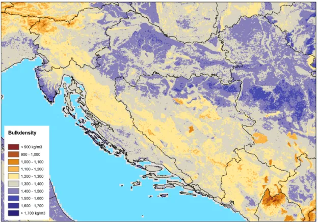
3.4.4 Soil data

Soil textural data were derived from the ISRIC Soilgrids database

http://www.isric.org/content/soilgrids , supplemented with data from JRC’s European Soils Bureau. Pedotransfer functions applied on 1km soil texture data - originating from the HYPRES database (Wösten et al., 1999) - were used to obtain the Mualem-VanGenuchten soil hydraulic parameters used for soil water transport modelling in LISFLOOD.

(31)

Figure 16 Bulk density of the top soil (0-30 cm). Source: ISRIC Soilgrids database.

3.4.5 Reservoirs and Lakes

The location of hydropower and thermal stations is derived from various sources:

• information provided from ISRBC experts and national focal points; • information from the Stockholm Royal Institute of Technology (KTH); • information from Sava member states internet sources;

• GRanD database (Global Reservoir and Dam database) (2011); • Global Lakes and Wetlands Database (GLWD, Lehner & Doell, 2004)

For almost all reservoirs, only basic parameters as location and total volume of the reservoir are available. Many of the reservoir steering parameters had to be estimated. Some of the parameters were included in the calibration. The calibration of the model was done taking the reservoirs and current water use into account.

3.4.6 Irrigation

Current irrigated areas are derived from Wriedt et al (2009), who established a pan-European irrigation map based on regional pan-European statistics, a pan-European land use map and a global irrigation map. The map provides spatial information on the distribution of irrigated areas per crop type which allows determining irrigated areas at the level of spatial modelling units. The irrigation map was compiled in a two step procedure. First, irrigated areas were distributed to potentially irrigated crops at a regional level

(32)

(European statistical regions NUTS3), combining Farm Structure Survey (FSS) data on irrigated area, crop-specific irrigated area for crops whenever available, and total crop area. Second, crop-specific irrigated area was distributed within each statistical region based on the crop distribution given in our land use map. A global map of irrigated areas with a 5′ resolution was used to further constrain the distribution within each NUTS3 based on the density of irrigated areas. The constrained distribution of irrigated areas as taken from statistics to a high resolution dataset enables us to estimate irrigated areas for various spatial entities, including administrative, natural and artificial units.

Figure 17 Current irrigated areas in the Sava basin.

Furthermore, sources from where water is abstracted are taken into account. The percentage of the source of the abstracted water used for irrigation is given, either from:

• surface water • groundwater

• non-conventional sources (e.g. desalination plants)

These data are derived from the FAO/Aquastat website (http://www.fao.org/nr/water/aquastat/irrigationmap/index10.stm ), and in many cases only available at country scale (see below). Croatia apparently has regional data available.

(33)

Figure 18 Fraction of groundwater used for water abstraction (source: FAO/Aquastat)

3.4.7 Water demand, abstraction and consumption

Water demands for the livestock sector, energy production and cooling, and the manufacturing industry are derived from downscaled Eurostat data mainly, as described by Vandecasteele et al (2013). Disaggregation has been achieved using 100m land use data.

Estimating cooling water abstractions were based on data from thermal power stations selected from the European Pollutant Release and Transfer Register data base (E-PRTR). Energy water withdrawals and projections are based on energy consumption projections from Prospective Outlook on Long-term Energy Systems (POLES) (JRC).

Livestock water withdrawals are based on FAO livestock density maps (FAO, 2012), refined with actual livestock figures for 2005 (CAPRI, 2012). Specific water requirements per livestock type were defined, and are varied with daily.

Household and public sector water demands are derived from ongoing work of Bernhard (2015, in preparation), using Eurostat reported data, disaggregated with land use and population maps to water use per capita. Projections include the influence of GDP and water price, as well as intra-annual seasonal influences and tourism, based on the number of hotel nights booked in a region.

Actual consumption is lower than abstraction. The remaining water is assumed to flow back to the system. Consumption percentages are based on literature values for each sector. For thermal power-stations, the type of cooling plays an important role in the actual consumption (evaporation) of water.

(34)

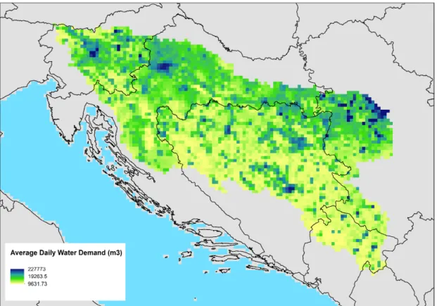
Figure 19 Average Daily Water Demand (m3 per 25km2 grid), for current climate and landuse.

Irrigation requirements are estimated inside the model – thus fully dynamically linked to changing precipitation and temperature, and thus adapting itself inside the climate scenario runs.

At a daily timescale, the difference between the potential evapotranspiration – depending on the weather forcing and crop requirements - and the actual evapotranspiration – based on soil moisture availability in addition – is taken as an estimated of the required irrigation water gift.

(35)

4. Descriptions of the scenarios

Below, the various scenarios are described for which the results are presented in Ch. 5.

4.1 Scenarios of future climate

Besides the baseline 1990-2013 observed weather data run, LISFLOOD has been run with a series of climate projections to evaluate the impact of future climate, combined with land use and measures such as irrigation, on water resources and extreme events. EURO-CORDEX bias corrected climate projections from the following sources were used:

• KNMI (Royal Netherlands Meteorological Institute) (NL) • SMHI (Swedish Meteorological and Hydrological Institute) (SE) • DMI (Danish Meteorological Institute( (DK)

• IPSL (Laboratoire des Sciences du Climat et de l'Environment) (FR)

From each of those main climate models, the following scenarios were used

• 1981-2010 (Historical) • RCP4.5 2011-2100 • RCP8.5 2011-2100

The hydrological model LISFLOOD is then run for the historical period 1981–2010 and for the future climate scenarios 2011–2040 and 2071-2100 forced by both RCP4.5 and RCP8.5 using the bias-corrected daily precipitation, average temperature and the generated potential evapotranspiration maps.

4.1.1 Comparison of climate control runs with observed weather data

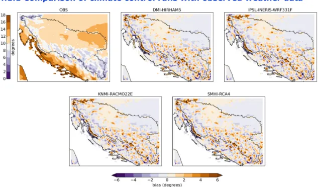
Figure 20 Average daily mean observed surface temperature (OBS) for the period 1990-2010 and the bias as simulated by the 4 RCMs.

(36)

It should be noted, that even though bias-correction using the E-obs gridded dataset has been applied, there are difference between the 1981-2010 historical (control climate) runs from those 4 suppliers and the gridded observed precipitation 1990-2012 which we use as observed weather, as can be seen in the figures below. Differences are mainly visible in the mountainous areas. Bias correction could be improved if better quality precipitation data would be available. The ongoing JRC funded extended CARPATCLIM project covering the Sava countries is aiming to achieve this improvement.

Figure 17 shows the bias of the average daily mean surface (2 meter) air temperature for each of the 4 RCMs for the period 1990-2010. In the same picture, the observed temperature is shown for reference, which is based on the JRC gridded meteorological data set (Ntegeka et al., 2013) for the same period. Similar scattered patterns of both warm and cold biases are found amongst the different RCMs. Warm biases up to 8o can mostly be found in the mountainous regions.

Figure 21 Average daily mean observed precipitation (OBS) for the period 1990-2010 and the bias as simulated by the 4 RCMs.

Figure 18 shows the bias in daily precipitation as modeled by the RCMs. The RCMs are in good agreement and are in general drier compared to the observations and extremely dry in mountainous regions. According Christensen et al. (2010) this is due to a lack of cloudiness modeled by the RCMs in this part of Europe. On the contrary the number of precipitation days (>0.1mm) modelled by the RCMs (Fig. 19) is higher compared to the observations. This turns out in less dynamic behavior of the RCMs in precipitation compared to observations with. Probably this is due to the fact that the relevant role of land-atmosphere interactions (e.g., convection) in summer is underestimated by the RCMs.

(37)

Figure 22 Average yearly mean observed (OBS) number of rain days (>0.1mm) for the period 1990-2010 and the bias as simulated by the 4 RCMs.

4.1.2 Evaluating RCP4.5 and RCP8.5 climate projections for the Sava

In this section an analysis is made of the end of the century (2071-2099) climate change signal of both the RCP4.5 and RCP8.5 emission scenarios relative to present climate (1981-2010) as simulated by the RCMs. Figure 20 shows the temperature change at the end of the 21st century. In both scenarios and for all the 4 RCMs an increase in temperature is observed with values ranging between 0 and 2 degrees for the RCP4.5 scenario and up to 7 degrees for the RCP8.5 scenario. The most pronounce temperature increase is likely to be in the southeast part of the Sava catchment.

In general, all models project an increase in precipitation for the end of the 21st century for both the scenarios. Although the SMHI-RCA4 model projects a decrease in precipitation in the coast lines for the RCP8.5 scenario, a common feature in the RCMs is the slight increase in precipitation between the RCP4.5 and RCP8.5 scenario. The inter-model variability is in general small with the exception of the IPSL-INERIS-WRF2331F model which projects much larger precipitation amounts compared to the other three RCMs.

The climate signal in terms of the number of precipitation days is more diverse and with opposite trends between the different RCMs. Figure 22 shows the change in number of precipitation days larger than 0.1 mm with some models (DMI-HIRHAM5, KNMI-RACMO22E and partially also IPSL-INERIS-WRF331F) projecting a slight increase in the number of precipitation days and others (SMHI-RCA4) a decrease for the RCP4.5 scenario. For the RCP8.5 scenario an opposite trend is observed with most models projecting a decrease in the number of precipitation days up to 25 days per year. Looking at the more extreme events the climate projection show an increase in the number of precipitation days larger than 20 mm for all the RCMs and both the climate scenarios (Fig. 23).

Summarized, it is expected according the climate projections that both the temperature and precipitation amount will increase at the end of the 21st century. Most likely the

(38)

increase in temperature triggers convection in summertime resulting in heavy precipitation events.

Figure 23 Average daily temperature change as simulated by the RCM’s at the end of the century (2071-2099) for both the RCP4.5 and RCP8.5 scenario. The temperature change

(39)

Figure 24 Average daily precipitation change as simulated by the RCMs at the end of the century (2071-2099) for both the RCP4.5 and RCP8.5 scenario. The temperature change

(40)

Figure 25 Average daily change in the number of precipitation days (>0.1mm) as simulated by the RCMs at the end of the century (2071-2099) for both the RCP4.5 and

RCP8.5 scenario. The temperature change is relative to the present RCM reference climate (1981-2010).

(41)

Figure 26 Average daily change in the number of precipitation days (> 20mm) as simulated by the RCMs at the end of the century (2071-2099) for both the RCP4.5 and

RCP8.5 scenario. The temperature change is relative to the present RCM reference climate (1981-2010)

(42)

4.2 Scenarios of future land use

At present, project land use data are only available for EU28 countries, thus including Slovenia and Croatia. The other countries of the Sava basin are not yet included. Work is underway to establish land use projections for Serbia, Bosnia and Herzegovina and Montenegro as well. Therefore, in this study, urban and forest area in Serbia, Bosnia and Herzegovina and Montenegro are kept as in 2006. In the increased irrigated area scenarios, shifts are introduced from rainfed agriculture towards irrigated agriculture. With regard to Croatia, three significant changes are immediately apparent (see Figure 1). On the one hand, forest areas are expected to increase substantially between 2010 and 2050 until 50% of the country’s modelled land surface is forested; while on the other hand, areas of arable land and semi-natural vegetation are expected to decrease substantially. Industrial and urban land uses are expected to increase by respectively 22% and 1%, but the total effect is relatively minor due to the relatively small area that those land-uses occupy in 2010.

The trend in forest area between 2006 and 2050 depends, among other factors, on the projected afforestation/deforestation rates, based on country data reported in the frame of UNFCCC (country declarations). The main driver for the agricultural uses is the CAPRI model, which indeed forecasts a decrease in arable land.

Figure 27 Projected land use changes in Croatia from 2010 towards 2050 (Source: JRC LUISA model, version 2015)

(43)

Figure 28 Change in forested area by 2050 as compared to 2006, simulated by the LUISA model (Source: JRC 2015).

With regard to Slovenia the expected land-use changes are roughly similar: again, the LUISA modelling results demonstrate a substantial increase of forested area between 2010 and 2050 at the expense of arable land and semi-natural vegetation (see Figure 2). In fact, the area of semi-natural vegetation is almost completely gone by 2050 according to these results. The slight decrease in arable land is consistent with the projections provided by the CAPRI model results that are fixed inputs for LUISA. Compared with Croatia, growth in urban and industrial land uses has a more clearly noticeable impact on land-use patterns in Slovenia. Urban land use is expected to increase by roughly 22%; industrial land use is expected to increase by roughly 27%.

(44)

Figure 29 Projected land use changes in Slovenia from 2010 towards 2050 (source: JRC LUISA model).

Figure 30 Change in urban area in 2050 as compared to 2006, as simulated with the LUISA model.

For this study, the following land use scenarios will be used in the scenario combinations:

• Baseline land use 2006 • Land use 2010

• Land use 2030 • Land use 3050

(45)

4.3 Scenarios of increased irrigation

For crop irrigation, a number of scenarios have been defined:

- Baseline 2006: irrigated areas as in 2006, with optimum crop irrigation water gift.

- Increase of irrigation including the areas indicated by FAO as “equipped for irrigation” (available from FAO Aquastat), added with planned Worldbank funded irrigation areas in Bosnia Herzegovina and Montenegro (information from ISBRC national facilitators) (referred to in this study as ‘MaxIrrigation’)

- A variation of the previous ‘MaxIrrigation’ scenario, using increased abstraction from groundwater, and reduced abstraction from reservoirs and surface water (referred to in this study as ‘MaxIrrigationLZ’)

- Hypothetical scenario by which all current maize arable land is irrigated if weather and soil conditions require to obtain maximum possible maize production (referred to as ‘EpicMax’).

Figure 31 Maximized irrigation while using areas mentioned by FAO/Aquastat as equipped for irrigation.