Dyna, year 80, Nro. 180, pp. 4-8. Medellin, August, 2013. ISSN 0012-7353
MULTIPLICATIVE SINGLE NEURON HYBRID MODEL
PRONÓSTICO DE LA DEMANDA DE ELECTRICIDAD
USANDO UN MODELO HÍBRIDO SARIMA-NEURONA SIMPLE
MULTIPLICATIVA
JUAN DAVID VELÁSQUEZ HENAOProfesor Titular, Escuela de Sistemas, Universidad Nacional de Colombia, Medellín, [email protected] VIVIANA MARIA RUEDA MEJIA
Analista de Información, XM S.A. E.S.P., Medellín, [email protected] CARLOS JAIME FRANCO CARDONA
Profesor Titular, Escuela de Sistemas, Universidad Nacional de Colombia, Medellín, [email protected]
Received for review September 07th, 2012, accepted April 22th, 2013, fi nal version July, 12th, 2013
ABSTRACT: The combination of SARIMA and neural network models are a common approach for forecasting nonlinear time series. While the SARIMA methodology is used to capture the linear components in the time series, artifi cial neural networks are applied to forecast the remaining nonlinearities in the shocks of the SARIMA model. In this paper, we propose a simple nonlinear time series forecasting model by combining the SARIMA model with a multiplicative single neuron using the same inputs as the SARIMA model. To evaluate the capacity of the new approach, the monthly electricity demand in the Colombian energy market is forecasted and compared with the SARIMA and multiplicative single neuron models.
KEYWORDS: SARIMA; artifi cial neural networks; time series prediction; energy demand; energy markets; nonlinear models.
RESUMEN: La combinación de modelos SARIMA y redes neuronales son una aproximación común para pronosticar series de tiempo no lineales. Mientras la metodología SARIMA es usada para capturar las componentes lineales en la serie de tiempo, las redes neuronales artifi ciales son aplicadas para pronosticar las no-linealidades remanentes en los residuos del modelo SARIMA. En este artículo, se propone un modelo simple no lineal para el pronóstico de series de tiempo obtenido por la combinación de un modelo SARIMA y una neurona simple multiplicativa que usa las mismas entradas del modelo SARIMA. Para evaluar la capacidad de la nueva aproximación, la demanda mensual de electricidad en el mercado de energía de Colombia es pronosticada y comparada con los modelos SARIMA y la neurona simple multiplicativa.
PALABRAS CLAVE: SARIMA; redes neuronales artifi ciales, predicción de series de tiempo, demanda de energía; mercados energéticos; modelos no lineales.
1. INTRODUCTION
Forecasting nonlinear time series is a common application for artificial neural networks [1]. An approach for building hybrid methods with artifi cial neural networks is to suppose that a nonlinear time series is composed of linear and nonlinear components as follows [3,5,7]:
• = ! + " (1)
where denotes the original time series, ! is the non-stationary linear component and " is the nonlinear
component. Usually, the Box-Jenkins methodology [2] is used to specify ! as an (seasonal) ARIMA model and to calculate the residuals of the time series as:
# = • − !% (2)
An artifi cial neural network is used to approximate the nonlinear component " . By using this simple idea, several approaches have been proposed: Zhang [3] and Aladag et al. [7] use the SARIMA model residuals as inputs for an artifi cial neural network; while a multilayer perceptron neural network is used in [3], and Elman’s recurrent neural network is used in [7];
Tseng et al. [5] use the residuals and the forecasts • ! of a SARIMA model as inputs of multilayer perceptron. The rationale of these approaches is that the •! component (the ARIMA model) is able to represent the linear components in the time series as the trend or seasonal patterns, while the "! component captures the remaining nonlinearities in the data.
In all previous works [3,5,7], the fi rst stage consists of obtaining the specifi cation of a SARIMA model. In the second stage, the parameters (and fi tted residuals) of the SARIMA model remain fi xed while only the parameters of the artifi cial neural network are estimated.
However, previous approaches have two limitations: Firstly, the parameters of the hybrid model (1) are not optimal because the parameters of the SARIMA and the artifi cial neural network are not estimated simultaneously. Secondly, the confi guration (inputs, processing layers, and number of neurons for layer) of the artifi cial neural network is done by a trial and error process [8] [9].
In the next section, we propose a new hybrid model to overcome these limitations. In Section 3, an application case is presented. In Section 4, we summarize the results.
2. PROPOSED HYBRID MODEL
In the generalized single multiplicative neuron (GSMN) model [4], the current value of a time series is obtained as a function of previous values:
(3)
#! = "! = $ %&(')#!−)+ ,)) .
)=1
/
Where $(0) is the activation function and is the order of the nonlinear autoregressive model. We chose this model for the following reasons:
a) The specifi cation process of a GSMN corresponds to selecting only the appropriate lags of the time series modeled. For the standard multilayer perceptron, the specifi cation is more diffi cult: it is necessary to specify the number of hidden layers and the number of neurons per layer in addition to the appropriate lags.
b) The GSMN require fewer parameters than the standard multilayer perceptron and it has a better generalization capability as is demonstrated in the empirical evidence presented in [4]. As a consequence, a fewer number of iterations of the optimization algorithm are necessary to converge to the optimum of the loss function.
In our approach, we fuse a SARIMA model with a GSMN using the same inputs as the SARIMA component. Thus, we specify the GSMN model as:
(4) "!= $ %&(')#!−)+ ,)) )∈Φ &5067!−6+ 869 6 ∈Θ − 1/
where: Φ is the set that contains the same lags of #! used for the SARIMA model; Θ is the set that contains the same lags of 7! used for the SARIMA model; and $(0) = tanh 0 .
In (4), the term 5067!−6 + 869 is introduced with the aim of representing the nonlinear dynamics of the moving average component. Note that when we impose the restrictions ') = 06 = 0 and ,) = 86 = 1 , then
"! = tanh %&(0 ∙ #!−)+ 1) )∈Φ &50 ∙ 7!−6+ 19 6 ∈Θ − 1/ = tanh %& 1 )∈Φ & 1 6 ∈Θ − 1/ = tanh 0 = 0
and the proposed model is reduced to the SARIMA approach.
The proposed approach is a general nonlinear model for time series forecasting. The SARIMA component (•!) is a well-established and understood method for dealing with the linear components of the time series and allows for the modeler to represent characteristics such as the trend or seasonal patterns. The GSMN component (4) captures the remaining nonlinearities present in the data, which are not captured by the SARIMA methodology. The steps for building the model are described as follows:
Stage 1. Scaling: we scale the time series • in the interval [−1, +1] due to the limitation in the range of
"(#) = tanh # .
Stage 2. Linear modeling: We obtain the specifi cation of a SARIMA model for the time series using a well-established methodology. In other words, we specify the $ model. In this stage, the lags for • and & are obtained.
Stage 3. Nonlinear modeling: We use the same inputs (lags) as the SARIMA model, obtained in Stage 2, for specifying the GSMN model described in (4). All the parameters of the hybrid model (1) are optimized simultaneously (including the parameters of the SARIMA model) by minimizing the conditional sum of the squared residuals (SSE) calculated as:
SSE = ' &2, with & = • − $ − * (6)
using a gradient-based optimization technique. Due to the presence of local optimum points, it is necessary to realize several runs of the optimization algorithm with different initial values for the parameters of the model. For each run, initial values for the hybrid model are specifi ed as follows:
• For the linear model (SARIMA), we use the optimal parameter values calculated in Stage 2. • For the GSMN model, the initial values are random
following a uniform probability distribution with
-., #/ ∈ [−3, 3] and 4., 5/ ∈ [1 − 3, 1 + 3]; we
found that for 3 = 0.1, the optimization algorithm works fi ne.
In our case, we prefer the Broyden-Fletcher-Goldfarb-Shanno (BFGS) optimization algorithm.
3. ELECTRICITY DEMAND FORECAST
The proposed hybrid method is applied to forecast the monthly electricity demand (in GWh) in the Colombian Energy Market for the period from August 1995 (1995:8) to April 2010 (2010:4). All the models are estimated for the natural logarithm of the time series, but the measured forecasting errors are expressed in
terms of the original data. The fi rst 155 observations were used for fitting the models and the last 24 observations for evaluating their forecasting ability; we use two forecast horizons: from 2008:5 to 2009:4 (12 months) and from 2008:5 to 2010:4 (24 months). For both horizons, we calculate one month ahead of forecasts. For each model fi tted, we compute the mean absolute deviation (MAD) and the root of the mean squared error (RMSE).
In [10], the Box-Jenkins methodology [2] is applied to obtain a SARIMA model for this time series using the same fi tting and forecasts periods. A SARIMA (0,1,3) x (1,1,2)12 is the preferred model when the auto.arima() function in the “forecast” package of Hyndman and Khandakar [11] is used for the automatic selection of the best confi guration. The auto.arima() function implements a heuristic step-wise procedure for searching the confi guration of a SARIMA model that minimizes the Akaike information criterion. In Table 1, we reproduce the error measures reported in [10] for the fi tting and forecast periods.
The proposed specifi cation methodology is applied as follows:
Stage 1. The transformed time series (using the natural logarithm function) is scaled to the interval [-0.93, 0.93].
Stage 2. The Box-Jenkins methodology is applied to obtain a SARIMA model. In our case, it is the SARIMA (0,1,3) x (1,1,2)12 model reported in [10].
Stage 3. The SARIMA (0,1,3) x (1,1,2)12 model can be written as: (1 − 8)(1 − 812)(1 − 9 12812)• = : + (1 + ;18 + ;282+ ;383)(1 + >1812+ >2824)& (7)
By expanding both sides of the previous equation, we found that the lags for the autoregressive and moving average components are Φ = {1, 12, 13, 24, 25} and
Θ = {1, 2, 3, 12, 13, 14, 15, 24, 25, 26, 27}; see equation (4).
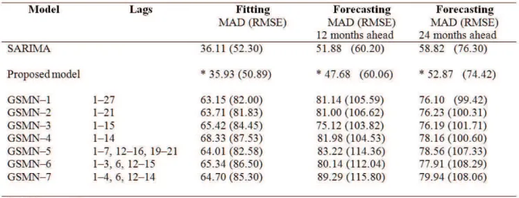
Table 1. Calculated errors
The final values of the parameters for the hybrid model are calculated by simultaneously optimizing the parameters of the SARIMA and GSMN components. The parameters are estimated by minimizing the conditional sum of squares of fitted residuals for
• = 28, … ,155 and !1= !2= ⋯ = !27= 0.
Also, we fi t several GSMN models, as defi ned in (3), to the transformed and scaled time series. The parameters are estimated by minimizing the conditional sum of squares of fi tted residuals for • = # + 1, … ,155 and !1= ⋯ = !#= 0 , where # is the maximum lag considered in the inputs of each model. The MAD and RMSE values for all models are s ummarized in Table 1. By analyzing the statistics reported in Table 1, we conclude that the proposed hybrid model is able to forecast the values of the studied time series with better accuracy. In Figure 1, we plot the real values of the time series and the forecasted values calculated using the proposed model.
4. CONCLUSIONS
In this paper, we discuss a new hybrid model obtained by fusing a SARIMA model and a generalized single neuron model. The proposed model has several advantages: fi rst, it is able to the capture nonlinear behavior in the data; second, the SARIMA approach provides the modeler with a well-known and accepted methodology for model specifi cation; and third, it is not necessary to use heuristics and expert knowledge for selecting the confi guration of the artifi cial neural network because the GSMN model uses the same inputs as the SARIMA model and it is not necessary to specify processing layers as in other neural network architectures. To assess the effectiveness of our model, we forecast the monthly demand of electricity in the Colombian energy market using several competitive models and we compare the accuracy of forecasts. The results obtained show that our approach performs better than the SARIMA and GSMN models in isolation. However, further research is needed to gain more confi dence and to better understand the proposed model.
REFERENCES
[1] Zhang, G., Patuwo, E.B. and Hu, M.Y., Forecasting with Artifi cial Neural Networks: the State of the Art. International Journal of Forecasting: 14 (1), pp. 35-62, 1998.
[2] Box, G.E.P. and Jenkins, G., Time Series Analysis, Forecasting and Control. Holden-Day, San Francisco, CA, 1970.
[3] Zhang, G.P., Time Series Forecasting using a Hybrid ARIMA and Neural Network Model. Neurocomputing: 50, pp. 159 – 175, 2003.
[4] Yadav, R.N., Kalra, P.K. and Jhon. J., Time Series Prediction with Single Multiplicative Neuron Model. Applied Soft Computing: 7(4), pp. 1157-1163, 2007. [5] Tseng, F.-M., Yu, H.-C. and Tzeng, G.-H., “Combining Neural Network Model with Seasonal Time Series ARIMA Model”. Technological Forecasting & Social Change: 69 (1), pp. 71-87, 2002.
[6] Khashei, M. and Bijari, M., An Artifi cial Neural Network (p, d, q) Model for Time Series Forecasting. Expert Systems with Applications: 37 (1), pp. 479-489, 2010.
[7] Aladag, C.H., Egrioglu, E. and Kadilar, C., Forecasting Nonlinear Time Series with a Hybrid Methodology. Applied Mathematics Letters: 22 (9), pp. 1467-1470, 2009.
[8] Kaastra, I. and Boyd, M.m., Designing a Neural Network for Forecasting Financial and Economic Time Series. Neurocomputing: 10 (3), pp. 215-236, 1996.
[9] Masters, T., Practical Neural Network Recipes in C ++. Academic Press, New York, 1993.
[10] Vega, W., Velásquez, J.D. and Franco, C.J., Forecasting the Monthly Electricity Demand in the Colombian Energy Market using an SARIMA Model. Technical Report, Escuela de Sistemas, Universidad Nacional de Colombia, 2010. [11] Hyndman, R.J., and Khandakar, Y., Automatic Time Series Forecasting: The Forecast Package for R. Journal of Statistical Software (2008) 27 (3), 2008.