Development Of Model For Supplier Selection And Order Allocation
With Discount Pricing And Expected Quality Loss
M. Imron Mustajib
Manufacturing Systems Laboratory Department of Industrial Engineering,
University of Trunojoyo Madura Jl. Raya Telang PO Box 2.
Bangkalan, Indonesia. Email: [email protected]
Abstract —This paper discusses the development of
optimization model for supplier selection and order allocation considering price discounts and quality of the components that are measured based on expectation of quality loss cost. The approach which was used quadratic loss function to estimated quality loss. The development of model is based on the drawback of previous research; where quality was measured only by defective components without considered to any loss of quality due to deviation from quality characteristics target. In the section of results and discussion of this paper is presented a numerical example in order to illustrate the implementation of proposed model. This numerical experiment performed by optimization software has indicated that the model able to generated optimal solution.
Keywords- optimization model, supplier selection, price, discount, quality loss
I. INTRODUCTION
Today's business competition not only involves competition among companies, but more extensive than it has involved competition among supply chain networks comprising: suppliers, manufacturers, warehouses, distributors, retailers and also raw materials and WIP flow in manufacturing facilities. There are several factors that are used as a competitive strategy to win the business competition in a dynamic environment namely [1]: quality, cost reduction, on-time delivery, and flexibility. Therefore, four factors must be considered in the early stage of the design of supply chain system as supplier selection process. Supplier selection methods have been developed in many literatures. According to Ordoobadi and Wang [2] there are at least 12 methods have been widely used. One of the methods of supplier selection is by using mathematical programming models. In general, mathematical models can select the supplier by considering constrains which are exist in the system to maximize or minimize the objective function the selection suppliers. The uniqueness of supplier selection based on mathematical models of obtained decision variables can be proved of it optimality.
In the perspective of mathematical programming, quality, cost, and delivery time factor (QCD) can be
formulated in a comprehensive manner to obtain optimal solutions for supplier selection process. For example the quality factor can be assessed with some aspects [3]:
1. Rate of rejects.
2. Continous improvement programs. 3. Quality of customer supports and services. 4. Certifications.
5. Percentage on-time shipments. 6. Technical and design level. 7. Easy of repair.
8. Reliability
9. Capability of handling abnormal quality. 10. Yield rate.
11. Process capability indices. 12. Loss function.
While the cost factor may involve a combination of some of the relevant costs in the system as well as the assumptions used. Among them are manufacturing cost, ordering or setup cost, purchasing cost, transportation cost, inventory cost and handling cost. Meanwhile, order delivery time is often calculated based on manufacturing lead time and transportation time.
The model suitability of supplier selection then will depend on three criterias [4]: the complexity of the situation and problems, the available information on supplier performance measures, and the interests of situation. In previous work by Feng et al. [5] proposed a stochastic integer programming (SIP) model for simultaneous tolerances and suppliers based on criteria of minimum production costs, which consists of manufacturing cost and expected loss cost of based on the concept of Taguchi's quality loss function. The tolerance limits of the specifications is set by the customer to choose component tolerances and suppliers. In the study, Feng et al. [4] not considered delivery time of orders to customer. Therefore, Irianto et al. [6] proposed an optimization process design based on the criteria of minimum production cost by considered tolerance delivery time limit specified by customer. The model was implemented manufacturing network in make-to-order (MTO) and engineering-to-order (ETO) environment. Futhermore, Irianto and Rachmat [7]
developed a model for process selection in make-to-order manufacturing network, which consists of: suppliers, manufacturers, and subcontractors by considering appraisal cost and time for inspection, correction and finishing.
Meanwhile, Shin et al. [8] proposed a probabilistic model where the cost of supplier quality performance is measured by non-conforming of components and performance expectations are estimated by the inappropriateness shipping delivery times either in the form of earliness and tardiness. Recently, Sawik [9] proposed a model of single and multiple objectives (many purposes) to select suppliers in make-to-order manufacturing systems based on price and quality of purchased components and reliability of delivery time. Sawik [9] recommended defects and unreliability of supply risk is controlled by the maximum number of delivery patterns, which is defect interval average or delivery rate is acceptable. In this study also considered price discounts offered by suppliers.
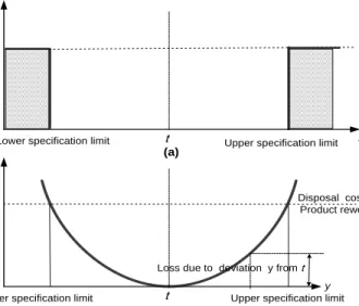
On the other hand, Tsai and Wang [10] proposed a model which is different from previous models. Tsai and Wang [10] used mixed integer programming approach to determine optimal supplier along with order allocation with diverse components and many suppliers in the supply chain. In that model the delivery time and quality factor calculated based on percentage of inaccuracies with the schedule and defect. Furthermore, they are compared some of usual discount schemes offered the supplier and its influence on purchasing decisions. However, Tsai and Wang [10] did not observe that any deviation from its target quality characteristic may cause quality loss cost, although still within quality specifications. This is inconsistent with the concept of quality as defined by Taguchi in Taguchi et al. [11] as the minimum product loss imparted by the society from the time the product shipped. Loss due to characteristic quality of components cannot meet consumer needs and satisfaction. Taguchi argues that there is a loss (in the form of a quadratic form of quality costs, see fig. 1.b) when quality characteristic deviating from the target, although the deviation is still within the specifications or the specified tolerances. The losses arise because of waste, loss of opportunity (opportunity cost) and cost when components fail to meet the specified target value of quality characteristics. This is clearly different from the traditional concept of view that each quality characteristic in the range specification does not cause loss of quality, as seen in the graph in fig.1.a.
Based on the absence of quality loss in the work of Tsai and Wang [10], this paper proposes an optimization model of supplier selection and order allocation considering expected quality loss based on quadratic quality loss function, which was recommended by Taguchi in Taguchi et al. (2005). The quality characteristic discussed in this paper is assumed nominal is the best.
Further discussion in this paper is organized as follows. Firstly, in the second section will explain the research method, which is deal with the development of
L(y)
y t
A
Lower specification limit
L(y)
y t
A Disposal cost or
Product rework
Loss due to deviation y from t Upper specification limit (a)
(b)
Lower specification limit Upper specification limit
FIGURE 1. (A) STEP LOSS FUNCTION, (B) QUADRATIC LOSS FUNCTION mathematical model formulation. Secondly, the third section discusses the results of model implementation and an analysis based on numerical example. To summarize in the fourth section of this paper will be given the conclusion of the model development and the results.
II. METHOD
In this paper, the decision making framework of supplier selection and order allocation depicted in fig. 2. Three main entities are included: set of suppliers, manufacturer, and costumers. Make-to-Order (MTO) Manufacturer has three main internal activities, namely: procurement, fabrication and assembly. The department of procurement is responsible for purchasing components from supplier alternatives. The problem of procurement decision is how to determine proper supplier and to allocate order of components. The main objective of procurement decision in this paper is to procure components at minimum cost with fit quality specification and on-time delivery to meet costumers demand. Finished product Fabrication Assembly Make-To-Order Manufacturer Set of Suppliers Procurement Minimize total costs Supplier’s Component 1 Supplier’s Component j Supplier’s Component J Customers Legend: Physical flow Information flow Determine quality and delivery time for each supplier alternatives
FIGURE 2. SUPPLIER SELECTION AND ORDER ALLOCATION FRAMEWORK
In order to determine quality level of components supplied by supplier alternatives, this paper proposes Taguchi quadratic loss function (see fig 1.b) as the calculation of quality loss cost that can be written by equation (1): 2 ) ( ) (y k y L y (1) with 2 y r y t C k (2) y
k is a constant to converting engineering characteristic to be cost characteristic, which ky is the coefficient of components quality loss that are estimated based on rework cost (Cr) needed when the quality characteristic y deviates
from the target product but still within the acceptable limits of customer tolerance (ty). When the condition of quality
characteristics is nominal the best by
the expected value of quality loss can be written as follows:) ) ( ( )] ( [ y y2 y y 2 y EL y k QL (3)
The variance (2y) in eq. 3 reflects the interval precision manufacturing process, while the bias ((yy)2) reflects the accuracy of the measurement result of manufacturing process.Biases can be reduced by reducing quality loss by adjustment of parameter μ at the design stage. Furthermore, expected quality loss of product (y) in eq. 3 is equal to the amount of quality loss of the ith component which is ordered from the jth supplier in the kth discount interval:
If the limit of the permitted deviation is 6σ, then one-side tolerance limit is considered, the quality variance of the ith component ordered from the jth suppliers with the kth price discount interval can be written:
2 2 3 ijk ijk t (5)
Furthermore, expectation of product quality loss (y) in eq. 3 is equal to the amount of quality loss the ith component, which is ordered from the jth supplier in the kth price discount interval:
I i J j K k ijk i y y t x y k y L E QL 1 1 1 2 2 3 )] ( [ (6) A. Model notationThe notations used troughout are given bellow. i. Indexes:
i : ith component.
j : jth supplier.
k : kth price discount interval
I : Set of components
J : Set of suppliers
K : Set of price discount intervals ii. Decision variables:
Xijk : quantity of the ith component ordered from
the jth supplier at the kth price discount interval
Yijk : the ith component ordered from the jth
supplier at the kth price discount interval. Yijk
equal to 1 if selected; 0, otherwise.
Zij : the ith component ordered from the jth
supplier. Zij equal to 1 if selected; 0,
otherwise. iii. Performance:
TC : total cost. iv. Parameters:
pijk : unit price for the ith component ordered from
the jth supplier at the kth price discount interval
dijk : discount coefficient for the ith component
ordered from the jth supplier at the kth price discount interval
y : quality characteristic of product, y=f (x1,..
xi,..xI)
i x
y
: partial derivative of the product functional quality with respect to the ith component.
ky : estimated quality loss coefficient of the
product.
tijk : quality tolerance for the ith component
ordered from the jth supplier at the kth price discount interval.
ty : quality tolerance of the product.
wijk : percentage of the ith component ordered from
the jth supplier at the kth price discount interval missing the scheduled delivery time.
lijk : penalty cost of the ith component ordered
from the jth supplier at the kth price discount interval due to missing the scheduled delivery time.
Di : aggregate demand for the ith component.
cij : capacity for the ith component ordered from
the jth supplier.
qijk : quantity at which quantity discount of the ith
component ordered from the jth supplier at the kth price discount interval
ni : maximum number of supplier that can be
selected for the ith component.
B. Model formulation
The entire results of the model development is formulated as follows. First, the objective function (eq. 7) is minimizing total cost which is consist of purchasing cost of components bought from supplier at specific discount interval, quality loss cost of product, and penalty cost
I i J j K k ijk ijk ijk y y E L y k QL 1 1 1 2 2 )] ( [ (4)related to lateness of delivery time schedule. Second, all the constaints of the system are steted in eq. 8 to eq. 16.
I i J j K k ijk ijk ijk ijk I i J j K k ijk i y I i J j ij ij I J j K k ijk ijk ijk X l w X t x y k Y f X p d TC Min 1 1 1 1 1 1 2 2 1 1 1 i 1 1 3 1 (7) Subject to: i I i i J j K k ijk D X
1 1 1 (8) j i ij K k ijk C X
, , 1 (9) k j i ijk ijk ijk ijk ijk Y X q Y q 1 , , , (10)
K k j i ij ijk Z Y 1 , , (11) 2 1 1 1 2 2 y ijk I i J j K k ijk i t X t x y
(12) i i J j ij n Z
, 1 (13)
i j ij Z 0,1, , (14) k j i ijk X 0, , , (15)
i j k ijk Y 0,1, , , (16)Constraint in eq. 8 secures demand fullfilment. Eq. 9 states order quantity is limited by the capacity of each suppliers. Contraint in eq. 10 indicates that order quantity must be at intervals of discounts offered. Constraint in eq. 11 represents only one discount interval selected in the selected supplier. Meanwhile, constraint 5 in eq. 12 ensures that each of components quality tolerance meet product quality specification. Eq. 13 states number of suppliers included for each components. Eq. 15 ensures order quantitity to all selected suppliers for each component positive integer. Constraints in eq. 14 and 16 impose binary requirement on the Zij and Yijk variables.
III. RESULTSANDDISCUSSION
In this section a numerical example is presented for the implementation of proposed model. The product example is one-way clutch (fig. 3), which are consisting of components:
1. Hub (x1), purchased from suppliers.
2. Roller ball (x2), produced by own manufacturer.
3. Cage (x3), purchased from suppliers.
The quality characteristic of one-way clutch is identified as the contact angle y, which is associated between the vertical line and the center of two rollers and the hub. In order to be able to operate normally, the contact angle must be maintained at 10.447 rad angle tolerance. Furthermore, the relationship between the contact angle y with the dimension of x1, x2, x3 can be expressed by equation:
2 3 2 1 3 2 1, , cos x x x x arc x x x f y (17) If known that :x155,306mm,x222,860mm,andx3101,900mm, then the partial derivative value of the contact angle y with respect to the dimensions of components x1, x2, x3 areobtained: mm rad x x x x x x x y / 1046 , 0 2 / 1 2 2 3 2 1 1 2 3 1 1 (18) mm rad x x x x x x x x x y / 2085 , 0 1 ) ( 2 / 1 2 2 3 2 1 2 2 3 1 3 2 (19) mm rad x x x x x x x x x y / 1046 , 0 1 ) ( 2 / 1 2 2 3 2 1 2 2 3 2 1 3 (20)
Meanwhile, the data of suppliers are obtained from Tsai and Wang [10] by adding the data of purchased component types and its quality tolerance of one-way clutch components as listed in Table 1. It is given that the quality loss coefficient is 50, the penalty cost of missing the scheduled delivery time is 50, the coefficient of price discount is 0.05 (k-1), k = 1, ... K, and the maximum number of suppliers to be choosed are two suppliers for each components.
TABLE 1. COMPONENTS AND SUPPLIERS DESCRIPTIONS
FIGURE 3. ONE-WAY CLUTCH (MODIFIED FROM [12]). Furthermore, the model optimization process carried out by using Lingo software to obtain the optimal decision variables. The optimal solution shows that the hubs are supplied from second supplier for 191 units and from third supplied for 309 units. Manwhile, the cages are supplied from second supplier for 80 units and from third suppliers for 420 units. The total cost obtained is 149,812.3.
IV. CONCLUDINGREMARKS
Today's business competition not only involves competition among companies, but also among supply chain networks. In the early stages of supply chain network
design, supplier selection is a key success to win in the competition. Quality, cost reduction, timely on-time delivery, and flexibility factors are the strategy, which are often considered for selecting suppliers. However, in previous studies the product quality is only measured by defect rate. It’s were not addressed any deviation from the quality characteristic target may causes the quality loss cost, although it still within quality specification limits.
Based on the drawbacks of previous research, this paper proposed a model for supplier selection and order allocation optimization considering price discounts and quality of the components that are measured based on expected quality loss cost. The approach used to estimate the quality loss is by using quadratic loss function. In order to validate proposed model it is presents numerical test performed by software. The result of numerical test indicates that the model can generates optimal solution.
REFERENCES
[1] Hallgren, M., and Olhager, J., (2006), “Differentiating Manufacturing Focus”, International Journal of Production Research, vol.44, no. 18-19, pp.3863-3878. [2] Ordoobadi, S.M., and Wang, S., (2011), “A Multiple Perspectives Approach to Supplier Selection”, Industrial Management and Data Systems, vol. 111, no. 4, pp. 629-648.
[3] Sadigh, A.N., Zulkifli, N.B., Hong, T.S. and Abdolshah, M., (2009), “Supplier Evaluation and Selection using Revised Taguchi Loss Function”,
Orde ring % of Late Tole rance Price pe r
Compone nt De mand Supplie r Capacity Cos t De live ry of Quality unit
p111=15 if 0≤x111≤85 1 800 550 1 0,5 p112=14,5 if 85≤x112≤180 p113=14 if x113≥181 p111=17 if 0≤x121≤95 1 (hub) 500 2 900 480 1,5 0,24 p122=16,5 if 95≤x122≤190 p123=16 if x123≥190 p131=13 if 0≤x131≤120 3 1200 600 4 0,1 p132=12,5 if 120≤x132≤200 p133=12 if x133≥200 p211=5 if 0≤x211≤70 1 1200 550 2 0,5 p212=4,5 if 70≤x212≤150 p213=4 if x213≥150 p221=3 if 0≤x221≤80 2 (cage) 500 2 900 480 5 0,27 p222=2,5 if 80≤x222≤160 p223=2 if x223≥160 p231=7 if 0≤x231≤125 3 1800 600 3 0,1 p233=6,5 if 125≤x232≤210 p233=6 if x233≥210
Journal of Applied Science, vol. 9, no. 44, pp. 4240-4246
[4] De Boer, L., Labro, E. and Morlacchi, P., (2001), “A review of Methods Supporting Supplier Selection”, European Journal of Purchasing & Supply Management, no. 7, pp. 75-89.
[5] Feng, C.X., Wang, J., and Wang, J.S., (2001), “An Optimization Model for Concurrent Selection of Tolerances and Supplier, Computer & Industrial Engineering, vol. 40, pp. 15-33.
[6] Irianto, D., Makmoen, M., and Taroepratjeka, H., (2004), “Pengembangan Model Optimasi Biaya, Kualitas dan Delivery untuk Sistem Manufaktur Berbasis MTO-ETO”, Jurnal Teknik dan Manajemen Industri, vol. 24, no. 1, pp. 1-6.
[7] Irianto, D., and Rahmat, D., (2008), “A Model for Optimizing Process Selection for MTO Manufacturer with Appraisal Cost”, Proceedings of the 9th Asia Pacific Industrial Engineering & Management Systems Conference, pp. 220-225.
[8] Shin, H., Benton, W.C., and Jun, M., (2009), “Quantifying Suppliers' Product Quality and Delivery Performance: A Sourcing Policy Decision Model”, Computer & Operation Research, vol. 36, pp. 2462-2471.
[9] Sawik, T., (2010), “Single vs. Multiple Objective Supplier Selection in Make to Order Environment”, Omega: The International Journal of Management Science, vol. 38, pp. 203-212.
[10] Tsai, W. C., and Wang, H.C., (2010), “Decision Making of Sourcing and Order Allocation with Price Discounts” Journal of Manufacturing Systems, vol. 22, pp. 47-54.
[11] Taguchi, G., Chowdhury, S., and Wu, Y., (2005), Taguchi’s Quality Engineering Handbook, John Willey & Sons. inc., Hoboken, NJ.
[12] Singh, P.K., Jain, S.C., and Jain, P.K., (2006) “Concurrent Optimal Adjustment of Nominal Dimensions and Selection of Tolerances Considering Alternatives Machines”, Computer-Aided Design, vol. 38, pp. 1074-1087.