Graph-based Coupled Behavior Analysis:
A Case Study on Detecting Collaborative
Manipulations in Stock Markets
Yin Song and Longbing Cao
Faculty of Information TechnologyCentre for Quantum Computation and Intelligent System (QCIS) Advanced Analytics Institute (AAI)
University of Technology, Sydney, Australia Email: [email protected], [email protected]
Abstract—Coupled behaviors, which refer to behaviors having some relationships between them, are usually seen in many real-world scenarios, especially in stock markets. Recently, the coupled hidden Markov model (CHMM)-based coupled behavior analysis has been proposed to consider the coupled relationships in a hidden state space. However, it requires aggregation of the behavioral data to cater for the CHMM modeling, which may overlook the couplings within the aggregated behaviors to some extent. In addition, the Markov assumption limits its capability to capturing temporal couplings. Thus, this paper proposes a novel graph-based framework for detecting abnormal coupled behaviors. The proposed framework represents the coupled behaviors in a graph view without aggregating the behavioral data and is flexible to capture richer coupling information of the behaviors (not necessarily temporal relations). On top of that, the couplings are learned via relational learning methods and an efficient anomaly detection algorithm is proposed as well. Experimental results on a real-world data set in stock markets show that the proposed framework outperforms the CHMM-based one in both technical and business measures.
I. INTRODUCTION
Human behavior (interchangeable with ‘behavior’ in this paper) refers to an action from a human and usually is coupled with behaviors of his/her own and other actors. ‘Coupled’ in this paper means behaviors have certain relationships and not independent. The couplings within an actor can be de-fined as intra-coupled relationships (‘intra-couplings’) while inter-coupled relationships (‘inter-couplings’) are between be-haviors of different actors [1]. Taking the couplings into account for anomaly detection is critical in many real-life scenarios whereas most of existed behavior analysis methods simply ignore these coupled relationships or only consider part of them (please see II for a brief review). Take the behaviors of investors in stock markets for example. ‘Place a buy order’ (‘buy’ for short), ‘place a sell order’ (‘sell’ for short) and ’generate a trade’ (‘trade’ for short, as an effect of matching a buy against a sell) are three typical trading behaviors. Intuitively, these behaviors are heterogeneous and not independent. In other words, if these trading behaviors are abnormal, they are coupled with each other and analyzing them individually cannot uncover the anomaly underlying
these coupled behaviors. (please see Section III-A for further details about how manipulations are coupled with each other.). Analyzing such kind of behavioral anomaly should not ignore these characteristics.
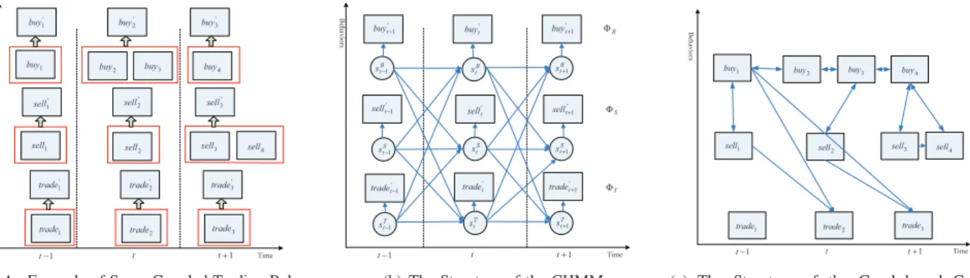
Recently, the group-based coupled behavior analysis (CBA) [1] was proposed to provide an innovative framework to com-prehensively analyze both intra- and inter-couplings between behaviors of a group of actors. As an initial attempt, the group-based CBA suggests a method to implicitly represent the couplings in a statistical model, coupled hidden Markov model (CHMM) [2]. For instance, suppose there are some trading behaviors as depicted in Fig. 1(a), where buyi(1 ≤ i ≤ 4),
selli(1 ≤ i ≤ 4) and tradei(1 ≤ i ≤ 3) denote the
corre-sponding ‘buy’, ‘sell’ and ‘trade’ behaviors. To capture the couplings between these behaviors, [1] proposed to generate homogenous time intervals using a sliding window and aggre-gate these behaviors according to the time intervals. As can be seen from Fig. 1(a), buyi,selli and tradei are converted to the corresponding aggregated behaviors buy′i, sell′i and
trade′i. On top of that, three chains ΦB (buy
′ 1,· · ·, buy ′ 3), ΦS (sell ′ 1,· · ·, sell ′ 3) and ΦT (trade ′ 1,· · ·, trade ′ 3) are
con-structed and a CHMM is set up to model the coupling relationships between the above behaviors via the hidden state space. The structure of the CHMM is shown in Fig. 1(b). For each aggregated behavior at one time stampt (i.e.,buy′t,
sellt′ and trade
′
t) there are corresponding hidden states to each behavior (i.e.,sB
t,sSt andsTt). The coupled relationships betweenbuyt′,sell
′ t,trade ′ tandbuy ′ t−1,sell ′ t−1,trade ′ t−1are
reflected in the dependency of the hidden statessB
t,sSt,sTt and
sB
t−1,sSt−1,sTt−1(similar situations to other time stamps). This
is feasible to some extent and the underlying assumption is that coupled behaviors could be modeled as a CHMM process. This solution, however, has some limitations: e.g., segmentation and aggregation of the behaviors may lose important coupling information within these aggregated behaviors; The first order Markov assumption (i.e., only considers the couplings between the aggregated behaviors of the current and previous time stamps) may not be a good approximation of real coupled behaviors.
U.S. Government work not protected by U.S. copyright
WCCI 2012 IEEE World Congress on Computational Intelligence
To overcome these weaknesses of the CHMM-based CBA, this paper proposes a graph-based framework to capture richer coupled relationships between behaviors and detect anomaly. The framework mainly consists of three stages. The first stage is to represent the behaviors in a graph structure. Fig. 1(c) describes the proposed graph structure for representation of the coupled behaviors. It has two main advantages compared to the CHMM-based framework: firstly, the behaviors are not aggregated and this avoids the possible loss of coupled rela-tionship information in the aggregated behaviors; secondly, the coupled relationships are not limited to the temporal Markov assumption and in Fig. 1(c) the possible coupled relationships between behaviors are indicated by directed links. These links are generated by some behavioral properties of the behaviors (for further details, please refer to IV), which indicate possible coupled relationships. For example, the behaviors are made at neighboring time stamps or the behaviors are made by the investors belonging to the same branch. On the basis of this graph-based coupled behavior model, in the second stage, relational learning methods [3] are adopted to capture more comprehensive coupled relationships of the normal behaviors. After that, the third stage further detects abnormal coupled behaviors (e.g., manipulations in stock markets) using the learned coupling model of the normal behaviors.
A. Contributions
While the coupled behaviors can be found in many real-world fields, such as group-based manipulations in stock markets and criminal behaviors, only limited efforts have been done for such behavior analysis. In this paper, a novel graph-based CBA framework has been proposed and a case study is presented to detect abnormal coupled behaviors (manipu-lations) in stock markets under the proposed framework. The main contributions of this paper are summarized as following.
• The introducing of a graph-based representation for
coupled behavior analysis. More specifically, this paper has made a first attempt to explain and model coupled relationships between behaviors based on a graph-based stucture, to the best of our knowledge.
• We further explore how to learning the coupled
rela-tionships between behaviors in the graph-based CBA framework, including how to preprocess the transactional data and model the coupled relationships via relational learning. In addition, this paper also proposes the corre-sponding anomaly detection techniques.
• Extensive experiments on a real-world data set from an
Asian stock market have been done as a case study. From both the views of technical and business performance, the experiments explore the comparison of the proposed framework and the previous CHMM-based framework. Different anomaly scores are compared as well.
B. Structure of this paper
The rest of this paper is organized as follows. Firstly, related work is given in Section II. In Section III, the CBA problem is illustrated by a case study of detecting abnormal
coupled trading behaviors in stock markets and a CHMM-based framework is reviewed. Then section IV describes our proposed framework of representing the behaviors in a graph and modeling the Couplings via relational learning algorithms and how to perform anomaly detection within the framework. Experimental results on a real data set of Asian stock market are given in Section V. Section VI concludes this paper.
II. RELATEDWORK
Below we briefly list a few related fields of our work. Coupled behavior analysis and anomaly detection are closely related to this paper in the sense of solving similar problems while statistical relational learning (SRL) is related to this paper in terms of methodologies.
A. Coupled Behavior Analysis.
One closely related area is group-based CBA proposed by [1], [4]. From the perspective of CBA, there are intra- and inter- couplings relationships between behaviors, as mentioned in Section I. Most of existing researches on behavior studies, however, focus mainly on discovering intra-relationship be-tween behaviors. For example, frequent pattern mining [5], a popular data mining technique in market basket analysis and custom behavior analysis, only considers the intra-couplings. For example, frequent itemset mining [6], [7] only consider the intra-couplings within each single transaction. Similarly, frequent sequence mining [8], [9] only considers the intra-couplings within a behavioral sequence of an individual, resulting in absence of analyzing the coupled relationships between different behavioral sequences. A comprehensive analysis of intra and inter relationships is beyond most of the current individual behavior analysis techniques, to the best of our knowledge. As an initial attempt, [1], [4] suggested a CHMM-based framework and indicates the couplings in a hidden state space. Although its success to some extend, as mentioned before, it is limited by the coupling information loss because of the transformation of behavioral data (in order to suit the structure of CHMMs) and the Markov assumption. Thus, an alternative modeling strategy is necessary, which is one of the main motivations of this paper.
B. Anomaly Detection.
Another field related to this paper is anomaly detection [10]. According to [10], this paper could fall into the category of collective anomaly detection, which means a collection of related instance (i.e. behaviors in this paper) is anomalous with respect to the entire data set. Most work of this category only consider intra-coupled relationships, such as [11] and [12], which means the behaviors are analyzed individually for each actor. By contrast, this paper explores the anomaly not only in intra- but also inter-couplings. In addition, this paper is also operate in semi-supervised mode [10], assuming that only the normal class has been labeled for training. This is reasonable and applicable because the abnormal behavioral data is usually hard to obtain.
7LPH %H K D Y LR UV WUDGH
WUDGH WUDGH WUDGH WUDGH WUDGH VHOO VHOO VHOO VHOO VHOO VHOO VHOO
EX\ EX\ EX\ EX\ EX\ EX\ EX\ − W W W+
(a) An Example of Some Coupled Trading Behav-iors in Stock Markets
7LPH %H K D Y LR UV − W WUDGH WUDGHW + W WUDGH − W VHOO W VHOO VHOOW+ − W EX\ W EX\ + W EX\ % W V− 6 W V− 7 W V− % W V 6 W V 7 W V % W V+ 6 W V+ 7 W V+ − W W W+ % Φ 6 Φ 7 Φ
(b) The Structure of the CHMM
7LPH %H K D Y LR UV
WUDGH WUDGH WUDGH VHOO VHOO VHOO VHOO
EX\ EX\ EX\ EX\
−
W W W+
(c) The Structure of the Graph-based Coupled Behavior Model
Fig. 1. The Coupled Behaviors and The Corresponding Two Different Models
C. Statistical Relational Learning.
Traditional statistical machine learning approaches assume that a random sample of homogeneous objects is from single distribution and independent to others. However, the charac-teristics of real world data sets violate the above assumption more often than not. They usually are: (1) multi-relational, heterogeneous and semi-structured; (2) noisy and uncertain. To fill the gap between the real world and the traditional machine learning, SRL has been proposed and become increas-ingly concerned by both the academic and industrial fields [13]. Meanwhile, a newly emerging research area, statistical relational learning [13] has been exploring the dependence relationships in relational heterogeneous data, such as aca-demic networks and World Wide Web, which can be utilized in the setting of coupled behavior analysis. Most of the current relational learning focus on classification of instances, given the label of some instances. Generally speaking, there are two types of SRL models in terms of inference: individual inference [14], [15] and collective inference [16], [17], [18], [19]. While collective inference model, such as relational dependency networks (RDNs) [3], utilize the related instance to infer one instance’s label, individual inference models does not and thus getting rid of high computational collective inference. Individual inference models, such as relational Bayesian classifiers (RBCs) [15] and relational probability trees (RPTs) [14], [20], typically transform relational data into propositional form so that conventional machine learning techniques (e.g., Bayesian classifiers and probability tree) can be applied. In this paper, relational learning is used to learning the couplings between coupled behaviors on the basis of the graph representation.
III. PROBLEMFORMATION
A. A Case Study in stock markets
In stock markets, the trading transactions are made up of trading actions from investors on their desired securities at particular trading prices, volumes and time points. As a toy example, Table I excerpts several order transactions of some investors and the corresponding trades made by them in an
Asian stock market. Common sense tells us these transactional behaviors are not isolated but coupled with other in certain relationships that sometimes could be anomalous. In fact, domain knowledge experts have identified Investor (1) and (2) as cooperative manipulators in this excerpt dataset. Such sophisticated manipulators carefully place quotes with specific prices, volumes and times to maximize personal benefits. As can be seen from Table I, investor (2) first placed a large buy at 10:00:35 to mislead other buyers after his/her partner (1)’s sell. To confuse other investors, (2) further placed a sell at 10:01:23 while (1) placed a buy at 10:01:38. After that other investors such as (4) and (5) followed up by submitting buy quotes at the same price as (2)’s sell. In this way, investor (1) and (2) cooperate to mislead other investors and sell the stocks at a higher price. Thus, the trading behaviors are coupled with each other and the coupling relationships may become abnormal when manipulations happen. Analysis of such coupled behaviors is considered to be a vital point of detecting the anomaly exists in the stock markets. The next sections will review the formalization of the CBA problem.
B. Coupled Behavior Analysis Problem.
Suppose there are I actors, an actor i undertakes mi be-haviors bi1,bi2,· · ·,bim
i. Each actor i’s j
th behavior b
ij
is associated with a behavioral type T(bij) = t(b ij. Each
behavioral type t ∈T has a number of associated properties
Pt = (Pt
1, P2t,· · ·, Pnt)(n may vary for different t value). Thus, each behaviorbij is associated with a set of behavioral
property value (a vector) (pt1bij,· · ·, ptnbij) determined by its behavioral type tbij. Then a behavior feature matrix F M(b)
for all actors for a specific period of time can be represented as follows [1]: F M(b) = b11 b11 · · · b1m max b21 b21 · · · b2m max .. . ... . .. ... bI1 bI1 · · · bIm max . (1)
where mmax = max{m1, m2, . . . , mI} , and for each
TABLE I
ANEXPERT OF THE‘ORDER’AND‘TRADE’ RECORDS INSTOCK
MARKETS
(a) Examples of buy and sell orders Investor Time Direction Price Volume
(1) 09:59:52 Sell 12.0 155 (2) 10:00:35 Buy 11.8 2000 (3) 10:00:56 Buy 11.8 150 (2) 10:01:23 Sell 11.9 200 (1) 10:01:38 Buy 11.8 200 (4) 10:01:47 Buy 11.9 200 (5) 10:02:02 Buy 11.9 250 (2) 10:02:04 Sell 11.9 500
(b) Examples of the corresponding trades Investor Time Direction Price Volume
(4) 10:02:04 Buy 11.9 200 (5) 10:02:04 Buy 11.9 250 (2) 10:02:04 Sell 11.9 450
j ≤ mmax) is defined as ∅, which means no action. Thus,
the intra-couplings are reflected by the relationship between elements within one row of the above matrix, whereas the relationships between elements of different rows indicate the inter-couplings. Specifically, Actori’s behaviorbij are
intra-coupled with other behaviors of the same actor in terms of the corresponding function θi
k(·)(1 < j ≤ mi, k 6= j) and
inter-coupled with other actors’ behaviors in terms of the corresponding function ηi
k(·)(1 < k ≤ I, k 6= i), with
non-determinism.
Definition 1 (Coupled Behaviors): Coupled behaviorsb
re-fer to behaviors bi
1j1 and bi2j2 that are coupled in terms
of the relationship f(θi1i2
j1j2(·))((i1 = i2)∧ (j1 6= j2)) or
f(ηi1i2
i1i2(·))((i1 6= i2)∧(j1 6= j2)), where (1 ≤ i1, i2 ≤
I)∧(1≤j1, j2≤mmax).
Theorem 1 (Coupled Behavior Analysis (CBA)): The
anal-ysis of coupled behavior is to build the objective functiong(·)
under the condition that behaviors are coupled with each other by coupling functionf(·), and satisfy the following conditions:
f(·) :=f(θ(·), η(·)). (2)
g(·)|(f(·)≥f0)≥g0. (3)
The above definitions formalize the problem of CBA and give the roadmap to solve this issue. But in real-applications, identifying both functions θ(·) and η(·) and the coupling function f(·) is usually beyond the capability of current knowledge because of the inherent unobservable and non-deterministic properties of coupling relationships. For simplic-ity and efficiency, [4], [1] proposed a coupled CHMM-based approach to represent the coupling in the hidden state space, which will be reviewed in the following before the description of our proposed framework.
C. CHMM-based Coupled Behavior Modeling
CHMM [2] is a statistical model designed to model mul-tiple processes with coupled relationships and each process
is represented by a univariate or multivariate time series, which means the time interval between instances are uniform. Human behaviors (instances), though, may not meet the above condition of uniform time interval more often than not. Thus, the CHMM-based framework suggests to convert the coupled behaviors to sequences and then use sliding time window to aggregate the behavioral instances to cater for the utilization of CHMM [1], as indicated by Fig. 1(a).
In the case study of [1], they build three hidden Markov models (HMMs) [21] for one CHMM: HM MB for buy sequenceΦB,HM MS for sell sequenceΦS andHM MT for trade sequence ΦT, as shown in Fig. 1(b). One HM M can be denoted of a set of conditional probability densities (CPDs) in terms ofA, B, C, πas follows:λHM M = (A, B, π)
, where
B is the observation probability distribution conditioned on the hidden state and π is the initial hidden state distribution andA, C is the conditional probability density of the current hidden statest conditioned on the previous hidden statest−1
(i.e.,p(st|past)and the parent node ofstis onlyst−1), which
models the couplings between behaviors. Correspondingly, a CHMM modeling three trading sequences can be expressed as λCHM M = (A, B, C, π). Then, A CHMM-based CBA framework can be built based on the following mapping relationships [1]:
CBA problem→CHM M M odeling (4)
f(θ(·), η(·))→(A, B, C, π) (5)
Meanwhile, as pointed out before, in order to build CHMM for analyzing the anomaly underlies the coupled trading behaviors [4], [1] converts the transactional data into behavior sequences and aggregating them, which makes the data suitable for CHMM-based modeling. Arguably, this kind of conversion may lose the information of important coupled relationships between behaviors. Motivated by this end, in next section, we present a novel graph-based CBA framework for a better modeling of coupled behaviors.
IV. PROPOSEDFRAMEWORK
A. Preliminaries
As shown in Fig. 1(c), a group of coupled behaviors can be represented by a typed, attributed graphGB = (VB, EB). The nodes VB represent behaviors (e.g., buyi(1 ≤ i ≤ 4),
selli(1 ≤ i ≤ 4) and tradei(1 ≤ i ≤ 4)) and the edges
EB represent potential coupled relations among the behaviors (e.g., the directed edges in Fig. 1(c) and please refer to Section IV-B for how to generate them). Suppose we have a group of behaviors, each behaviorbi∈VB is associated with
a typeT(bi) =tb
i and each behavior typet∈Thas a number
of associated attributes Xt = (Xt
1,· · ·, Xmt) (X
t ⊂ X
, where X = {X1, X2,· · ·, Xn} is the whole attribute set
associated with the coupled behaviors: e.g., trading price, trading volume). An example can be seen in Fig. 2(b). There are no hidden variables in our proposed graph-based model and we directly model the couplings of behaviors by a set of CPDs of all the behavioral attributesXin a relational setting.
Specifically, for any specific attribute instance xi of Xi in a behavior b, the CPD p(Xi = xi|paxi) is conditioned on
the attribute values of other behaviors linked tob(as well as
other attribute values ofbitself). In this sense, the couplings
between behaviors are considered in the form of a set of CPDs (in a relational setting 1) for different behavioral attribute values of the coupled behaviors conditioned on related values (similar to the A, C of the CHMM framework). Then, A relational learning-based CBA framework can be built based on the following mapping relationships:
CBA problem→SRL M odeling (6)
f(θ(·), η(·))→p(Xi=xi|paxi), Xi∈X (7)
The following content describes how the proposed frame-work frame-works, which includes three stages: data preprocessing, modeling coupled behaviors via relational learning and the corresponding anomaly detection algorithm.
B. Data Preprocessing
Let us review the behavior feature matrix defined in Equa-tion 1, this feature matrix encodes all the behaviors that are coupled together for analysis. Intuitively, the space for analyze the couplings among these behaviors are almost infinite. For a coupled behavior bj in n coupled behaviors, it could be
possibly coupled to any one of the remainingn−1behaviors and the corresponding search space isO(Cn1−1). Generally, if
considering it to be coupled to any k, 1 ≤ k ≤ n−1, the possible search space could be O(Ck
n−1). Thus, if we sum
up the search space and the overall search space could be
O(2n−1), which means computational complex is exponential
to the increase of the number of coupled behaviors. This is intractable when the number of the coupled behaviors is large. Alternatively, we could limit the search space suggested by some reference behavioral properties of the behaviors indi-cating the possible coupled relationships. Then the remaining behavioral properties can be defined as analysis properties, which are used for learning the coupled relationships between the behaviors in terms of CPDs in a relational setting. The formal definition of such two properties is as following.
Definition 2 (Reference Property): A reference propertyR
refers to the behavioral property which is used to generate the possible underlying coupled relationships between behaviors, usually user-defined.
Definition 3 (Analysis Property): A analysis property A
refers to the behavioral property which is used to learn the coupled relationships between behaviors.
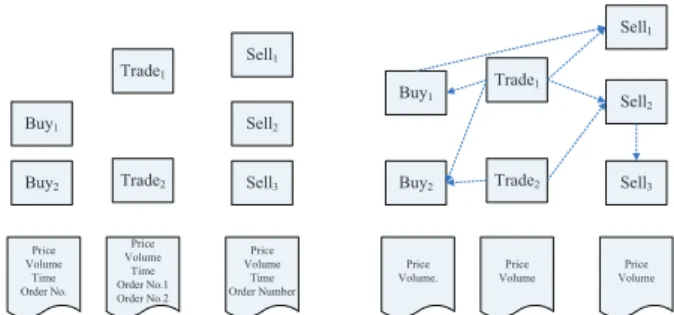
Let us see an example to clarify these definitions. Recall the Case Study in stock markets described in Section III. As mentioned above, there are three type of behaviors in stock markets: ‘buy’, ‘sell’ and ‘trade’. These behaviors are coupled with each other and exhibit different relationships which may indicate the manipulation of the market. As shown in Fig. 2(a). 1This CPD is not the same as the CPD in a flat setting which only consider the dependency of intrinsic attribute values (i.e., the attribute values within the same instance), for further details, please refer to [3].
Sell1 Sell2 Sell3 Trade1 Trade2 Buy1 Buy2 Price Volume Time Order No. Price Volume Time Order No.1 Order No.2 Price Volume Time Order Number
(a) The coupled behaviors with refer-ence and analysis properties
Sell1 Sell2 Sell3 Trade1 Trade2 Buy1 Buy2 Price Volume. Price Volume Price Volume
(b) Link generation using reference properties
Fig. 2. An example for illustration of reference and analysis properties
The three kinds of behaviors all have the corresponding behavioral properties. In terms of coupled behaviors, these properties can be divided into reference property (indicating possible couplings) and analysis property(for analysis of cou-plings under the constrain of possible coucou-plings). For example, in Fig. 2(a), the behavioral properties of ‘buy’ are: ‘Price’, ‘Volume’, ‘Time’ and ‘Order No.’. The reference property can be ‘Time’ and ‘Order No.’. The property ‘Time’ may become a clue of the coupled behaviors neighboring in time. This is reasonable because beyond the time constrain the behaviors have less chance to be coupled. Consequently, these possible coupled behaviors are linked for further analysis, as shown in Fig. 2(b). Similarly, another property ‘Order No.’ of ‘buy’ and ‘trade’ behaviors points out the corresponding ‘trade’ behaviors (also have order Numbers). These possible relationships are also generated in terms of links between the behaviors. Other links between these behaviors are generated as long as users are interested in such possible couplings.
C. Modeling Coupled Behaviors via Relational Learning
After obtaining the graph structure of the coupled behaviors, we further explore the learning of couplings between the behaviors (i.e., a set of CPDs.). In some cases, estimating all the CPDs may not be of the direct interest. For example, in stock markets, the ‘trade’ behavior directly influence the price of a specific security and the ‘buy’ and ‘sell’ behaviors have indirect impact on the price fluctuation. In other words, in stock market, the manipulators control the market through deliberately arranging the trading prices of the securities which are decided by ‘trade’ behaviors directly. To detect the anomaly in stock markets, we are more interested in modeling the fluctuation of ‘trade’ behaviors’priceattribute values and its dependency on other related trading behaviors’ attribute values. Thus, we alternatively model the CPD of theprice at-tribute values conditioned on other related behavioral atat-tribute values. Consequently, we need to specify the ‘target behavior’ (e.g., the ‘trade’ behaviors) and the ‘target behavioral property’ (e.g., the ‘price’ attribute) and their formal definition is as following:
Definition 4 (Target Behavior): A target behavior b(t)
i is
determined by its behavioral type tb(t) i
behav-TABLE II
ANEXAMPLE OF FLAT THE COUPLED BEHAVIORAL DATA
RF1 RF2 · · · RFn
trade1 rf11 rf21 · · · rfn1
trade2 rf12 rf22 · · · rfn2
ioral type of behaviors are indicated as target behaviors by prior domain knowledge.
Definition 5 (Target Behavioral Property): A target
behav-ioral propertyX
t
b(t)
i is usually one of the properties belonging
to one behavioral type and specified by prior domain knowl-edge as well.
In consequence, in order to model the coupled relation-ships among behaviors, we could estimate the CPD becomes
p(X
t
b(t)
i = x|pax)., underlies which the coupled relations
between behaviors are considered: To learn the p(Xtb(t) i =
x|pax)is challenging because the parent node of a behavioral attribute instance could be heterogenous. A possible method is to flat the parent nodes (the attribute values of linked behaviors) into relational features. [14], [15] and [3] proposed different strategies to flat data using relational features. For example, the ‘trade’ behaviors in Fig. 2(b) can be trans-formed into TABLE II by generating the relational features
RF1,· · ·, RFn.
a) Modeling of Conditional Probability Distribution:
Theoretically, any models learn the conditional probability distribution can be used for our task for coupled behaviors learning. Here we discuss two different conditional probability models: relational probability trees (RPTs) [14] and relational Bayesian classifiers (RBCs) [15]. The main differences be-tween the two methods are how to generate relational features and how to use them.
b) Relational Bayesian Classifiers: RBCs are simple
Bayesian classifiers to model relational data, which in this paper is coupled behavior data. Similar to the independence assumption of the naive Bayesian classifier, RBCs flat the relational data into propositional data through multiset esti-mators, such as average value, independent value and average probability [15]. For example, consider the ‘trade’ behavior as the target behavior and its price property as the target behavioral property in Fig. 2(b). To estimate the relational CPD for the attribute price values on behavior trade, the RBC considers all the attribute values associated with the related behaviors buy, sell, trade and treats them as inde-pendent relational features. The CPD can be estimated as
p(x|pax)∝p(x)p(rf1|x)p(rf2|x). . . p(rfn)(rf1 torfn refer
to the relational feature values). Please refer to [15] for further details.
c) Relational Probability Trees: An alternative way to
estimate the CPD by a RPT. The RPT algorithm uses aggre-gation functions (e.g, mode, count, proportion and degree) [14] to transform the relational feature to a propositional feature, which is different to the RBC algorithm. After that a probabil-ity tree is construct to select proper features to represent the desired CPD. For example, consider the ‘trade’ behavior as the
target behavior and its price property as the target behavioral property in Fig. 2(b). A possible if-then rule generated by the RPT could beif RF1> T0then p(price=price1) = 80%
(e.g.,RF1could be the average price of related buy behaviors
and T0 is a constant). A set of this kind of rules could
represent the CPD we want to estimate. In other words, the RPT algorithm automatically generates and selects aggregated relational features to model the CPD of the target behavioral property values (e.g., price values in Fig. 2(b)) of the target behavior (e.g., the trade behavior in Fig. 2(b)) conditioned on other related behavioral attribute values. Please refer to [14] for further details.
D. Abnormal Coupled Behaviors Detection
Having modeled the normal coupled behaviors, we must further determine whether the new coming coupled behaviors are normal or abnormal. An intuitive solution to this problem is to calculation the conditional likelihood (CL) given the observations of the coupled behaviors based on the normal model M (i.e. the CPD learned), which is CL(bk) =
Q
bi∈bkp(X
t
b(t)
i = x|rf1i, rf2i,· · ·, rfni;M). This can be
also used to predict the value of the target behavior property and then compared to the true value of the property. The obtained performance measure (e.g., area under ROC curve (AUC) and accuracy) can also be used to check how well the coupled behaviors are modeled by the normal model as well. Thus, in this paper, we integrate the performance measure and the corresponding CL value as the anomaly score for the coupled behaviors.
AS(bk) =CL(bk)∗AU C(bk)∗Accuracy(bk) (8)
The assumption is that abnormal trading behaviors are less likely to be predicted based on normal behaviors and have a low CL value.
The algorithm for detecting abnormal coupled behaviors is described in Algorithm 1. As shown in Algorithm 1, step 1 is train a normal model M0 of all the coupled behaviors in
the training set. Step 2 to 7 is a loop process to calculate the corresponding anomaly score of each group of coupled behaviors in the testing set. If the anomaly score is lower than some predefined threshold, the corresponding group of coupled behaviors is judged as anomaly. The output of this baseline algorithm is the set of anomaly.
V. EMPRICALRESULTS
A. The Data set
The experimental data set is from an Asian stock market. It covers 388 valid trading days from 1 June 2004 to 31 December 2005. The data is partitioned into two sets sug-gested by domain experts. The training data set consists of transactions collected from 1 June 2004 to 31 December 2004, by filtering those transactions associated with the identified alerts. We treat it as ’normal’ data. The remainder of the transactional data form the test set. The behavioral data of each trading day in the training and testing set can be seem
Algorithm 1Model-based Anomaly Detection Input: A Training set{b1,b2,· · ·,bN},
A Testing set{b1,b2,· · ·,bM},
A Model TypeM,
A ThresholdT h0.
Output: An anomaly setA.
1: Train oneM0 model on the training set{b1,b2,· · ·,bN,}.
2: for allbkin the Testing setdo
3: Compute the anomaly score of bk given the model M0:
AS(bk|M0) 4: ifAS(bk|M0)< T h0 then 5: bk→ A 6: end if 7: end for as bj (1 ≤j ≤ N) and bk (1 ≤k ≤ M) in Algorithm 1,
respectively. Those transactions with alerts are not removed from the test set so that the test set is made up of both normal and abnormal coupled trading behaviors. Alerts fired by the existing surveillance system are referred as rough benchmark for us to evaluate the performance of our proposed algorithm. Because it is very costly and time-consuming to label the data, the above evaluation method is suitable and reasonable.
B. Performance Measure
In this paper, we evaluate the performance of our pro-posed algorithms from both technical and business perspec-tive. True positive T P, true negative T N, false positive
F P and false negative F N are counted in terms of treat-ing the abnormal cases as the positive class. The technical performance of a framework is then evaluated by accuracy
( T P+T N T P+F N+F P+T N), precision ( T P T P+F P), recall ( T P T P+F N), and specificity ( T N
F P+T N). On the other hand, two business metrics, return and abnormal return [22], are used as indicators for abnormal dynamics surveillance of the market. Empirically, the trading days with exceptional patterns are more likely to incur a higher return and abnormal return than those without exceptional trading. Return refers to the gain or loss for a single security or portfolio over a specific period, which is calculated byReturn = lnptpt
−1, where pt and pt−1 are the
trade prices at timetandt−1, respectively. Abnormal return is defined as the difference between the actual return of a single security or portfolio and the expected return over a given time period. The expected return is the estimated return based on an asset pricing model, using a long-term historical average, or multiple valuations. The formula to compute abnormal return is as AbnormalReturn = Return−(γ+ξReturnmarket), where Returnmarket is the observed return for the market index, γ and ξ are the estimated parameters using previous return observations.
C. Comparison of Different relational models and the CHMM
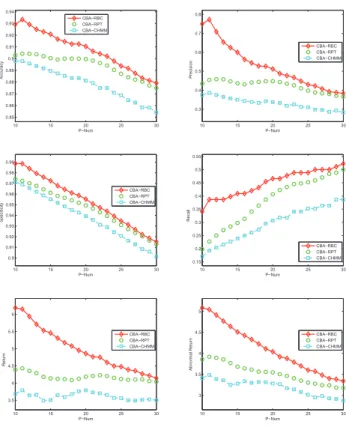
We tested the two different CBA framework based on two different relational models (denoted as RBC’ and ‘CBA-RPT’, respectively) on the test data set and compared them to the CHMM-based CBA framework (denoted as
‘CBA-10 15 20 25 30 0.85 0.86 0.87 0.88 0.89 0.9 0.91 0.92 0.93 0.94 P−Num Accuracy CBA−RBC CBA−RPT CBA−CHMM 10 15 20 25 30 0.3 0.4 0.5 0.6 0.7 0.8 P−Num Precision CBA−RBC CBA−RPT CBA−CHMM 10 15 20 25 30 0.9 0.91 0.92 0.93 0.94 0.95 0.96 0.97 0.98 0.99 P−Num Specificity CBA−RBC CBA−RPT CBA−CHMM 10 15 20 25 30 0.15 0.2 0.25 0.3 0.35 0.4 0.45 0.5 0.55 P−Num Recall CBA−RBC CBA−RPT CBA−CHMM 10 15 20 25 30 3.5 4 4.5 5 5.5 6 P−Num Return CBA−RBC CBA−RPT CBA−CHMM 10 15 20 25 30 3 3.5 4 4.5 5 P−Num Abnormal Return CBA−RBC CBA−RPT CBA−CHMM
Fig. 3. Technical and Business Performance of the Four Models
CHMM’)2. Fig. 3 shows both their technical performance. The horizontal axis (P-Num) stands for the number of detected group-based abnormal behaviors (of a trading day), and the vertical axis represents the values of technical measures (ac-curacy, precision, recall or specificity) or business measures (return and abnormal return). As can be seen from Fig. 3(a), Fig. 3(b), Fig. 3(c) and Fig. 3(d), both the two relational learning-based CBA frameworks perform better than the pre-vious proposed CHMM-based framework. Specifically, when
P−num= 11, the precision of the RBC-based framework can be100.02%higher than that of the CHMM-based framework. Simialr trends can be seen in other measures. This proves the data transformation in the CHMM-based framework may cause information loss and lead to poorer performance. Of the two relational models, the CBA-RBC performs the best in terms of all the measures. This is may be because the way the RBC constructs relational features are more close to the real situation in this case, compared to the RPT, which may be helpful to capture more comprehensive couplings between behaviors.
D. Exploration of Different Anomaly Scores
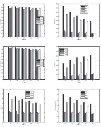
Here we compare four anomaly scores, denoted as ‘AS1’, ‘AS2’, ‘AS3’ and ‘AS4’, respectively. The ‘AS1’ is defined as in Equation 8, whileAS2(bk) =Accuracy(bk),AS3(bk) =
AU C(bk)andAS4(bk) =CL(bk). The experimental results
2The performance results are the averaged values of different time sliding windows [4].
10 15 20 25 30 0 0.1 0.2 0.3 0.4 0.5 0.6 0.7 0.8 0.9 1 P−Num Accuracy AS1 AS2 AS3 AS4 10 15 20 25 30 0 0.1 0.2 0.3 0.4 0.5 0.6 0.7 0.8 P−Num Precision AS1 AS2 AS3 AS4 10 15 20 25 30 0 0.1 0.2 0.3 0.4 0.5 0.6 0.7 0.8 0.9 1 P−Num Specificity AS1 AS2 AS3 AS4 10 15 20 25 30 0 0.1 0.2 0.3 0.4 0.5 0.6 0.7 P−Num Recall AS1 AS2 AS3 AS4 10 15 20 25 30 0 1 2 3 4 5 6 7 P−Num Return AS1 AS2 AS3 AS4 10 15 20 25 30 0 1 2 3 4 5 6 P−Num Abnormal Return AS1 AS2 AS3 AS4
Fig. 4. Technical and Business Performance of the Four Anomaly Scores
3on the data set is shown in Fig. 4. The horizontal and vertical axes in Fig. 4 have the same meanings of that in Fig. 3. From the picture, we can see our proposed anomaly score ‘AS1’ performs the best. An intuitive explanation is that ‘AS1’ consider the most comprehensive aspects to in the four scores for comparison.
VI. CONCLUSIONS
We introduce a challenging issue of detecting abnormal trading coupled behaviors and propose a graph-based CBA framework. The graph model avoids the data transformation and the Markov assumption in the previous CHMM-based framework, and is expected to have a more accurate modeling of the coupled relationships between the behaviors, which is helpful to further anomaly detection. In the case study of detecting abnormal trading behaviors in stock markets, we have demonstrated that the graph-based CBA framework performs better than the CHMM-based framework and the proposed anomaly score is effective compared to alternative scores. Additional research includes applying our proposed CBA framework to other scenarios, such as social security and social welfare data mining where people’s behaviors are also coupled with each other, and investigations on capturing the dynamics of the coupled relationships between normal behaviors which may change over time.
3Only the performance results of CBA-RBC are reported because of limited space and other models exhibit similar trends.
ACKNOWLEDGMENT
This work is sponsored in part by Australian Research Council Discovery Grants (DP1096218) and ARC Linkage Grant (LP100200774). We appreciate the comments and help provided by Dr. Yiling Zeng and Dr. Xiaodong Yue.
REFERENCES
[1] L. Cao, Y. Ou, and P. Yu, “Coupled behavior analysis with applications,”
IEEE Transactions on Knowledge and Data Engineering, 2011. [2] M. Brand, N. Oliver, and A. Pentland, “Coupled hidden markov models
for complex action recognition,” inProceedings of the1997 IEEE Com-puter Society Conference on ComCom-puter Vision and Pattern Recognition, 1997, pp. 994–999, cvpr.
[3] J. Neville, “Statistical models and analysis techniques for learning in relational data,” Ph.D. dissertation, 2006.
[4] L. Cao, Y. Ou, P. Yu, and G. Wei, “Detecting abnormal coupled sequences and sequence changes in group-based manipulative trading behaviors,” in Proceedings of the 16th ACM SIGKDD international conference on Knowledge discovery and data mining. ACM, 2010, pp. 85–94.
[5] J. Han, M. Kamber, and J. Pei,Data mining: concepts and techniques. Morgan Kaufmann Pub, 2011.
[6] R. Agarwal, C. Aggarwal, and V. Prasad, “A tree projection algorithm for generation of frequent item sets,”Journal of parallel and Distributed Computing, vol. 61, no. 3, pp. 350–371, 2001.
[7] J. Han, J. Pei, Y. Yin, and R. Mao, “Mining frequent patterns without candidate generation: A frequent-pattern tree approach,”Data Mining and Knowledge Discovery, vol. 8, no. 1, pp. 53–87, 2004.
[8] J. Han, J. Pei, B. Mortazavi-Asl, Q. Chen, U. Dayal, and M. Hsu, “Freespan: frequent pattern-projected sequential pattern mining.” ACM, 2000, pp. 355–359, proceedings of the sixth ACM SIGKDD interna-tional conference on Knowledge discovery and data mining.
[9] J. Han, J. Pei, B. Mortazavi-Asl, H. Pinto, Q. Chen, U. Dayal, and M. Hsu, “Prefixspan: Mining sequential patterns efficiently by prefix-projected pattern growth,” 2001, pp. 215–224, proceedings of the 17th International Conference on Data Engineering.
[10] V. Chandola, A. Banerjee, and V. Kumar, “Anomaly detection: A survey,”
ACM Computing Surveys (CSUR), vol. 41, no. 3, pp. 1–58, 2009. [11] C. Warrender, S. Forrest, and B. Pearlmutter, “Detecting intrusions using
system calls: Alternative data models,” inProceedings of the 1999 IEEE Symposium on Security and Privacy, 1999, pp. 133–145.
[12] P. Chan and M. Mahoney, “Modeling multiple time series for anomaly detection,” 2005.
[13] L. Getoor and B. Taskar,Introduction to statistical relational learning. The MIT Press, 2007.
[14] J. Neville, D. Jensen, L. Friedland, and M. Hay, “Learning relational probability trees.” ACM, 2003, pp. 625–630, proceedings of the ninth ACM SIGKDD international conference on Knowledge discovery and data mining.
[15] J. Neville, D. Jensen, and B. Gallagher, “Simple estimators for relational bayesian classifiers,” 2003.
[16] N. Friedman, L. Getoor, D. Koller, and A. Pfeffer, “Learning probabilis-tic relational models,” inInternational Joint Conference on Artificial Intelligence, vol. 16. Citeseer, 1999, pp. 1300–1309.
[17] B. Taskar, P. Abbeel, and D. Koller, “Discriminative probabilistic models for relational data,” inEighteenth Conference on Uncertainty in Artificial Intelligence (UAI02). Citeseer, 2002, pp. 895–902.
[18] M. Richardson and P. Domingos, “Markov logic networks,”Machine learning, vol. 62, no. 1, pp. 107–136, 2006.
[19] K. Kersting and L. De Raedt, “Basic principles of learning bayesian logic programs.” Citeseer, 2002, institute for Computer Science, University of Freiburg.
[20] J. Neville, . im ek, D. Jensen, J. Komoroske, K. Palmer, and H. Goldberg, “Using relational knowledge discovery to prevent securities fraud.” ACM, 2005, pp. 449–458, proceedings of the eleventh ACM SIGKDD international conference on Knowledge discovery in data mining. [21] L. Rabiner, “A tutorial on hidden markov models and selected
applica-tions in speech recognition,”Readings in speech recognition, vol. 53, no. 3, pp. 267–296, 1990.
[22] B. Brown Jerold and J. Stephen, “Using daily stock returns* 1:: The case of event studies,”Journal of financial economics, vol. 14, no. 1, pp. 3–31, 1985.