U
NIVERSITY OF
I
NSUBRIA
Department of Science and High TechnologyPh.D. course in Computer Science and Computational Mathematics (XXIX cycle)
Tikhonov-type iterative regularization
methods for ill-posed inverse problems:
theoretical aspects and applications
Author:
Alessandro BUCCINI
Supervisor:
iii
“I accept nothing on authority. A hypothesis must be backed by reason, or else it is worthless.”
v
UNIVERSITY OF INSUBRIA
Abstract
Department of Science and High Technology
Doctor of Philosophy
Tikhonov-type iterative regularization methods for ill-posed inverse problems: theoretical aspects and applications
by Alessandro BUCCINI
Ill-posed inverse problems arise in many fields of science and engineering. The ill-conditioning and the big dimension make the task of numerically solving this kind of problems very chal-lenging.
In this thesis we construct several algorithms for solving ill-posed inverse problems. Start-ing from the classical Tikhonov regularization method we develop iterative methods that enhance the performances of the originating method.
In order to ensure the accuracy of the constructed algorithms we insert a priori knowledge on the exact solution and empower the regularization term, thus keeping under control the ill-conditioning of the problems. By exploiting the structure of the problem we are also able to achieve fast computation even when the size of the problem becomes very big.
The methods we developed, in order to be usable for real-world data, need to be as free of pa-rameters as possible. For most of the proposed algorithms we provide efficient strategies for the choice of the regularization parameters, which, most of the times, rely on the knowledge of the norm of the noise that corrupts the data.
We construct algorithms that enforce constraint on the reconstruction, like nonnegativity or flux conservation and exploit enhanced version of the Euclidian norm using a regularization operator and different semi-norms, like the Total Variaton, for the regularization term. For each method we analyze the theoretical properties, like, convergence, stability, and reg-ularization. Depending on the method we are going to consider the finite dimensional case or the more general case of Hilbert spaces.
Numerical examples prove the good performances of the algorithms proposed in term of both accuracy and efficiency. We consider different kinds of mono-dimensional and two-dimensional problems, with a particular attention to the restoration of blurred and noisy images.
vii
Acknowledgements
First and foremost I would like to thank my supervisor Prof. Marco Donatelli for his contin-uous support during these three years of Ph.D.. He taught me a lot; not only he has allowed me to grow as a mathematician, but also as a person.
Thanks to all the people I had the privilege to work with: Zhong-Zhi Bai, Davide Bianchi, Pietro Dell’Acqua, Fabio Ferri, Ken Hayami, Ronny Ramlau, Lothar Reichel, Stefano Serra-Capizzano, Jun-Feng Yin, and, Ning Zheng.
I would also like to thank the referees Marco Prato and Lothar Reichel for their remarks, which have improved the quality and the readability of this Ph.D. thesis.
A special thanks to Lothar and Laura for their hospitality and kindness during my staying in Kent. You really made me feel at home!
Thanks also to Ronny for having me in Linz. It had been a wonderful time!
I would also wish to thank all theInsubria familywho has always been there when I needed
them most.
ix
Contents
Abstract v
Acknowledgements vii
List of Figures xi
List of Tables xiii
List of Abbreviations xv
List of Symbols xvii
1 Introduction 1 2 Background 7 2.1 Ill-posed problems . . . 7 2.1.1 Image Deblurring . . . 9 Boundary Conditions . . . 10 2.2 Tikhonov Regularization . . . 11
2.2.1 Tikhonov in general form . . . 13
2.2.2 Iterated Tikhonov . . . 15
3 Constrained Tikhonov Minimization 17 3.1 Reformulation of the problem . . . 18
3.2 Modulus Method . . . 19
3.3 Golub-Kahan bidiagonalization . . . 20
3.4 Krylov subspace methods for nonnegative Tikhonov regularization . . . 22
3.5 Numerical examples . . . 26
4 Iterated Tikhonov with general penalty term 35 4.1 Standard Tikhonov regularization in general form . . . 36
4.2 Iterated Tikhonov regularization with a general penalty term . . . 37
4.2.1 Convergence analysis for square matricesAandL . . . 38
4.2.2 Extension to rectangular matrices . . . 44
4.2.3 The nonstationary iterated Tikhonov method with a generalL . . . 44
4.3 Numerical examples . . . 46
5 Fractional and Weighted Iterated Tikhonov 53 5.1 Preliminaries . . . 54
5.2 Fractional variants of Tikhonov regularization . . . 58
5.2.1 Weighted Tikhonov regularization . . . 58
5.2.2 Fractional Tikhonov regularization . . . 60
5.3 Stationary iterated regularization . . . 62
5.3.2 Iterated fractional Tikhonov regularization . . . 64
5.4 Nonstationary iterated regularization . . . 66
5.4.1 Nonstationary iterated weighted Tikhonov regularization . . . 66
Convergence analysis . . . 66
Analysis of convergence for perturbed data . . . 75
5.4.2 Nonstationary iterated fractional Tikhonov . . . 76
Convergence analysis . . . 76
Analysis of convergence for perturbed data . . . 78
5.5 Numerical examples . . . 79
6 Approximated Iterated Tikhonov: some extensions 85 6.1 Approximated Iterated Tikhonov . . . 86
6.2 Approximated Iterated Tikhonov with general penalty term (AIT-GP) . . . . 87
6.3 Approximated Projected Iterated Tikhonov (APIT) . . . 96
6.3.1 Approximated Projected Iterated Tikhonov with General Penalty term (APIT-GP) . . . 98
6.4 Numerical Examples . . . 98
7 Multigrid iterative regularization method 105 7.1 Preliminaries . . . 106
7.1.1 Multigrid Methods . . . 106
7.1.2 Tight frames denoising . . . 109
7.2 Our multigrid iterative regularization method . . . 111
7.2.1 Coarsening . . . 111
7.2.2 Smoothing . . . 113
7.2.3 The algorithm . . . 114
7.3 Convergence Analysis . . . 115
7.4 Numerical Examples . . . 121
8 Weakly Constrained Lucy-Richardson 127 8.1 Physical details . . . 128
8.1.1 Discretization of the Fredholm Integral Equation . . . 129
8.1.2 Constraints . . . 130
8.2 An iterative method based on Lucy-Richardson method . . . 131
8.2.1 Heuristic interpretation . . . 133
8.2.2 Estimation ofγ . . . 134
8.3 Numerical Examples . . . 135
9 A semi-blind regularization algorithm 141 9.1 The regularized functional . . . 142
9.2 Constraints and flux conservation . . . 147
9.3 Minimization Algorithm . . . 150
9.3.1 ADMM . . . 150
9.3.2 The proposed Algorithm . . . 153
Proof of convergence . . . 156
9.4 Numerical examples . . . 163
10 Conclusions and Future work 173
xi
List of Figures
1.1 Schematic of the thesis . . . 5
2.1 Shawtest problem . . . 9
2.2 Examples of boundary conditions . . . 12
2.3 Peppers test problem . . . 14
2.4 Peppers test problem reconstructions . . . 14
3.1 Shawtest problem . . . 27
3.2 Grain test problem . . . 30
3.3 Grain test problem reconstructions . . . 30
3.4 Peppers test problem . . . 31
3.5 Peppers test problem reconstructions . . . 31
3.6 Atmospheric blur test problem . . . 33
3.7 Atmospheric blur test problem reconstructions . . . 33
3.8 Atmospheric blur test problem reconstructions detail . . . 34
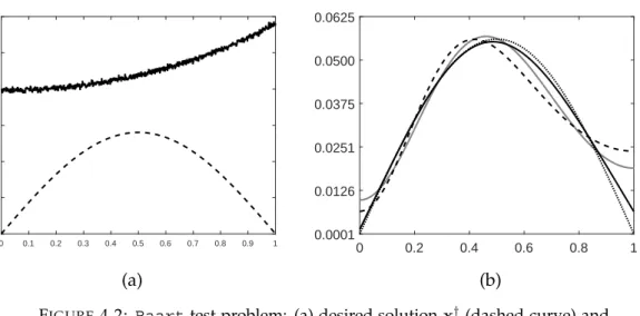
4.1 Stationary iterated Tikhonov regularization: RRE obtained different values ofα 47 4.2 Baarttest problem . . . 48
4.3 Baart test problem (supplementary material) . . . 49
4.4 Deriv2test problem . . . 50
4.5 Gravitytest problem . . . 50
4.6 Peppers test problem . . . 51
4.7 Peppers test problem reconstructions . . . 52
5.1 Foxgoodtest problem . . . 79
5.2 Deriv2test problem . . . 81
5.3 Blurtest problem . . . 82
5.4 Blurtest problem reconstructions . . . 83
6.1 Barbara test problem . . . 100
6.2 Barbara test problem reconstructions . . . 100
6.3 Grain test problem . . . 101
6.4 Grain test problem reconstructions . . . 102
6.5 Grain test problem detail of the error . . . 102
6.6 Satellite test problem . . . 102
6.7 Satellite test problem reconstructions . . . 103
6.8 Evolution of the relative reconstruction error against the iterations . . . 103
7.1 V-cycle scheme . . . 108
7.2 Grain test problem . . . 122
7.3 Grain test problem reconstructions . . . 123
7.4 Grain test problem: Error obtained with ADMM-UBC with respect to the reg-ularization parameter . . . 123
7.6 Cameraman test problem reconstructions . . . 125
7.7 Biological image test problem . . . 125
7.8 Biological image test problem reconstructions . . . 126
8.1 Normalized behavior of the kernelK(θ, R)and of the kernel amplitudeK(θ= 0, R) . . . 129
8.2 Discretization scheme of equation (8.1) . . . 130
8.3 Test 1: Comparison between the original LR and our WCLR algorithm . . . . 137
8.4 Test 2: Behavior as a function ofγof the average parametersRRE,DN, andDV137 8.5 Test 2: Comparison between the average recovered distributions with the true solution . . . 138
8.6 Test 3: Behavior as a function ofγof the average parametersRRE,DN, andDV139 8.7 Test 3: Comparison between the average recovered distributions with the true solution . . . 140
9.1 Boat test problem . . . 167
9.2 Boat test problem errors comparison . . . 168
9.3 Boat test problem reconstructions . . . 168
9.4 Example from [18] . . . 169
9.5 Example from [18] reconstructions . . . 169
9.6 Satellite test problem . . . 170
9.7 Satellite test problem reconstructions . . . 170
9.8 Grain test problem . . . 171
9.9 Grain test problem reconstructions . . . 171
9.10 Comparison of the norm of the iterates generated by CSeB-A with the pro-posed bounds for all the examples . . . 171
xiii
List of Tables
2.1 Peppers test problem . . . 13
3.1 Shawtest problem . . . 28
3.2 Shawtest problem . . . 29
3.3 Grain test problem . . . 30
3.4 Peppers test problem . . . 31
3.5 Atmospheric blur test problem . . . 32
4.1 Baarttest problem . . . 49
4.2 Deriv2test problem . . . 50
4.3 Gravitytest problem . . . 51
4.4 Peppers test problem . . . 52
5.1 Foxgoodtest problem (stationary case) . . . 80
5.2 Foxgoodtest problem (nonstationary case) . . . 81
5.3 Deriv2test problem (nonstationary case) . . . 82
5.4 Deriv2test problem (nonstationary case) . . . 82
5.5 Blurtest problem (nonstationary case) . . . 83
5.6 Blurtest problem (nonstationary case) . . . 83
6.1 Barbara test problem . . . 101
6.2 Grain test problem . . . 102
6.3 Satellite test problem . . . 103
7.1 Grain test problem . . . 122
7.2 Cameraman test problem . . . 124
7.3 Biological image test problem . . . 125
xv
List of Abbreviations
ADMM AlternatingDirectionMultiplierMethod AIT ApproximatedIteratedTikhonov
AIT-GP ApproximatedIteratedTikhonov withGeneralPenalty term APIT ApproximatedProjectedIteratedTikhonov
APIT-GP ApproximatedProjectedIteratedTikhonov withGeneralPenalty term CGLS ConjugateGradient method forLeastSquare problems
CSeB-A ComputationalSemiBlindADMM FlexiAT FlexibleArnoldiTikhonov
FOV FieldOfView
GIT IteratedTikhonov withGeneral penalty term
GITN S NonstationaryIteratedTikhonov withGeneral penalty term
GSVD GeneralizedSingularValueDecomposition
IT IteratedTikhonov
ITN S NonstationaryIteratedTikhonov
LCP LinearComplementarityProblem
LR Lucy-Richardson
LSQR LeastSquaresResidual method MvPs Matrix-vectorProducts
MgM MultigridMethod
MM ModulusMethod
NN-Restart-GAT NonnegativeRestartedGeneralizedArnoldiTikhonov NSIFT NonstationaryIteratedFractionalTikhonov
NSIWT NonstationaryIteratedWeightedTikhonov NNLS Nonnegative constrainedLeastSquares
NNQP Nonnegative constrainedQuadraticProgramming PDE PartialDifferentialEquation
PSF PointSpreadFunction
PSNR PeakSignal toNoiseRatio
RRAT RangeRestrictedArnoldiTikhonov RRE RelativeReconstructionError SeB-A SemiBlindADMM
SIFT StationaryIteratedFractionalTikhonov SIWT StationaryIteratedWeightedTikhonov SNR Signal toNoiseRatio
SVD SingularValueDecomposition
TwIST TwoStepsIterativeShrinkageThresholding WCLR WeaklyConstrainedLucy-Richardson wlsc WeaklyLowerSemi-continuous
xvii
List of Symbols
kxk1 1norm ofx
A∗ Adjoint operator (for matrices it denotes the conjugate transpose ofA)
argmin
x∈Ω
f(x) Argument of the minimum of the functionf(x)on the setΩ1
LA Augmented Lagrangian
x∗y Convolution betweenxandy
D(A) Domain ofA
A◦B Element-wise multiplication between matrices
kxk Euclidean norm ofx
∇sφ(s, t) Gradient ofφwith respect to the variables
H1 H1Sobolev space
X,Y Hilbert spaces
inf
x∈Ωf(x) Infimum of the functionf(x)on the setΩ 1
hx,yi Inner product betweenxandy
max
x∈Ω f(x) Maximum of the functionf(x)on the setΩ 1 min
x∈Ωf(x) Minimum of the functionf(x)on the setΩ 1 sup
x∈Ω
f(x) Supremum of the functionf(x)on the setΩ1
kxkT V Total Variation norm ofx
At Transpose ofA
PΩ Metric projection overΩ
A† Moore-Penrose Pseudoinverse ofA
N(A) Null space ofA
(x)+ Positive part ofx, i.e.,(x)+= max{x,0}
R(A) Range ofA
Re(x) Real part ofx
AΩ Restriction ofAonΩ
σ(A) Set of the singular values ofA λ(A) Spectrum ofA
∂sφ(s, t) Subdifferential ofφwith respect to the variables
1If
xix
To my parents, my family, and friends.
1
Chapter 1
Introduction
In this thesis we deal withill-posed inverse problems. This kind of problems arises in many
scientific fields from mathematics to physics and engineering. Solving these problems can be very difficult, but they present interesting challenges from both the theoretical and com-putational point of view; see [61] for more details about inverse problems.
There is no formal definition of inverse problems. Intuitively we are dealing with an inverse problem when we want to recover an object from some measured data knowing the process that generated the latter from the first.
We mainly consider problems that, when discretized, lead to linear system of equations. Be-cause the original problem is ill-posed the resulting linear system is severely ill-conditioned. In real applications, it is impossible to avoid the presence of noise in the data, i.e., the right-hand side of the system, so direct inversion leads to very poor reconstructions. These prob-lems usually have very large dimensions making the work at hand even more complicated. Moreover, to enhance the quality of the computed solution, we enforce constraints, like non-negativity, furtherly complicating the numerical methods involved in the solution of the problem.
Consider the case in which the operator to be inverted is compact. It is well known that the inverse of such an operator is unbounded. In particular, when the data is noise affected, the inversion process will amplify the noise to the point of corrupting the entire reconstruction making it completely useless.
In order to recover useful solutions, we need to resort to regularization methods, see e.g. [61, 78, 80]. Regularization methods substitute the original ill-conditioned problem with a well-conditioned one whose solution is a good approximation of the original. The accuracy of the recovered solution depends, at least in part, on how much information is available on the true solution and how this knowledge is inserted inside the algorithm itself.
The goal of this thesis is to develop several regularization methods for solving ill-posed inverse problems. For each of the algorithm proposed we give a theoretical analysis of their properties and show the performances on synthetic data.
The keystone of the methods we are going to develop is Tikhonov regularization which is described in Section 2.2. We are going to use the basic idea of Tikhonov regularization in order to formulate new and accurate iterative methods. The regularization effect will be obtained either by the knowledge of the limit point of such iterations or by the early stop of these by means of a suitable stopping criterion.
We are also going to consider strategies for achieving fast computations, either by exploiting the structure of the problem or by using linear algebra techniques, like Krylov methods, to compress the dimension of the problem without losing any relevant information.
The formulation of these new methods will be obtained by using the available knowledge on the exact solution and by improving the effectiveness of the regularization terms.
For testing the quality of our methods we will consider both one and two dimensional prob-lems. In particular, for most of this thesis, we are going to consider the case of image deblur-ring.
The task of recovering an image from a blurred version of itself is a classical application in the framework of inverse problems. The blurring phenomenon can be modeled as a Fredholm integral of the first kind where the kernel is compact and possibly smooth. This operator re-duces itself to a convolution operator when the blur is assumed to be spatially invariant, i.e., when the blur does not depend on the location. In the spatially invariant case the discretized operator can be represented by a highly structured matrix. In real case scenarios it is possible to have knowledge only over a finite region, the so called Field of View (FOV). In order to avoid underdetermined linear system it is necessary to make assumption on what is outside the FOV by means of the boundary conditions, see [84] for more details. The structure of the blurring operator is determined by the boundary conditions, but the basic structure is that of two level Toeplitz, i.e, a block Toeplitz with Toeplitz block matrix, where we recall that a Toeplitz matrix is a matrix whose entries are constant along the diagonals. This structure gives us the possibility ti exploit the Fast Fourier transform (FFT) to lower the computational effort of the algorithms. Moreover, Toeplitz matrices have been widely studied and thus we have a very deep knowledge of their properties.
In many situations it is known that the exact solution of the problem lies in some set. It might then be helpful to constrain the reconstructions to lie inside this set. In the case of image deblurring, for example, it is well known that the solution cannot attain negative value, so constraining the reconstruction to belong to the nonnegative cone can greatly improve the quality of the reconstruction. We are going to see that inserting this kind of knowledge inside the algorithms can enhance the quality of the reconstruction while having a very small impact on the computational cost.
This thesis is structured as follows
Chapter 2. Background In this chapter we give an insight on the basic concept of ill-posed problems. We formally introduce the image deblurring problem and explore some of his aspects, like the boundary conditions. We then describe the Tikhonov regularization method in both its standard and general form, where the regularization term is measured with a semi-norm usually defined by the discretization of a differential operator. Finally, we derive the iterated Tikhonov (IT) method as a refinement technique solving the error equation by Tikhonov regularization.
Chapter 3. Constrained Tikhonov Minimization As stated above, the introduction of a constraint inside the regularization can improve the quality of the reconstruction. In this chapter we analyze the case of nonnegatively constrained Tikhonov regularization. We re-formulate the problem at hand in a suitable way in order to be able to apply the Modulus Method (MM). This method let us compute the solution of the constrained problem. In order to reduce the computational effort, we use the Golub-Kahan bidiagonalization technique to project the problem into a Krylov subspace of fairly small dimension. In this way we are able to obtain a very fast method without losing anything in term of quality of the reconstruction. The contents of this chapter are based on [8].
Chapter 1. Introduction 3
Chapter 4. Iterated Tikhonov with general penalty term The theory of the IT method has been developed only in the case where Tikhonov in its standard form is considered. In this chapter we develop a theory for the IT algorithm where Tikhonov is considered in its general form. We consider both the stationary and nonstationary version of the algorithm. We analyze its convergence in the noise-free case and show that in the noisy case, if equipped with a suitable stopping criterion, this method is a regularization method. Comparison with the classical IT algorithm shows how much the usage of the general form helps in improving the quality of the provided reconstruction. This chapter is related to the paper [30].
Chapter 5. Fractional and Weighted Iterated Tikhonov In two recent works [86, 95] two extensions of the classical Tikhonov regularization method were introduced. We provide saturation and converse results on their convergence rate. We formulate, using a refinement technique, the related iterative method both in stationary and nonstationary version. We show that these iterated methods are of optimal order and overcome the previous saturation results. Furthermore, for nonstationary iterated fractional Tikhonov regularization methods, we establish their convergence rate under general conditions on the iteration parameters. Numerical results confirm the improvements obtained against the classical IT algorithm. The contents of this chapter are based on [14].
Chapter 6. Approximated Iterated Tikhonov: some extensions The nonstationary precon-ditioned iteration proposed in the recent work [49] can be seen as an approximated iterated Tikhonov method. Starting from this observation in this chapter we extend the previous iteration in two directions: the usage of Tikhonov in its general form, as suggested by Chap-ter 4, and the projection into a convex set (e.g., the nonnegative cone as suggested by the results in Chapter 3). Depending on the application both generalizations can lead to an improvement in the quality of the computed approximations. Convergence results and reg-ularization properties of the proposed iterations are proved. Finally, the new methods are applied to image deblurring problems and compared with the iteration in the original work and other methods with similar properties recently proposed in the literature. The contents of this chapter are taken from [26].
Chapter 7. Multigrid iterative regularization method Multigrid methods have been suc-cessfully used for solving linear systems coming from the discretization of PDEs for many years. It has been only in recent years that they have been considered for ill-posed prob-lems. Their regularization power has been discussed for the first time in [56]. In this chap-ter we construct a multigrid algorithm for image deblurring that combines both linear and non-linear methods. The grid transfer operator used for this method is able to preserve the structure of the operator across the levels making possible to achieve fast computations. We combine one of the algorithms described in Chapter 6 with Linear Framelet Denoising to regularize the problem while preserving the details of the image without amplifying the noise. We study the convergence of the algorithm under some restrictive, but reasonable, hypothesis and prove that, if provided with the suitable stopping criterion, it is a regular-ization method. The comparison with other methods from the literature proves that it is a very powerful method able to restore with high accuracy blurred image without having to estimate any parameter. The contents of this chapter are taken from [27].
Chapter 8. Weakly Constrained Lucy-Richardson Lucy-Richardson (LR) is a classical it-erative regularization method largely used for the restoration of nonnegative solutions. LR
finds applications in many physical problems, such as the inversion of light scattering data. In these problems, there are often additional information on the true solution that are usu-ally ignored by many restoration methods because these quantities are likely to be affected by non negligible noise. In this chapter we propose a novel Weakly Constrained Lucy-Richardson (WCLR) method in which we add a weak constraint to the classical LR by in-troducing a penalization term, whose strength can be varied over a very large range. The WCLR method is simple and robust as the standard LR, but offers the great advantage of widely stretching the domain range over which the solution can be reliably recovered. Some selected numerical examples prove the performances of the proposed algorithm. The con-tents of this chapter are taken from [28].
Chapter 9. A semi-blind regularization algorithm In many inverse problems the operator to be inverted depends on a parameter which is not known precisely. In this chapter, follow-ing the idea from [17,18], we propose a Tikhonov-type functional that involves as variables both the solution of the problem and the parameter on which the operator depends. We first prove that the non-convex functional admits a global minimum and that its minimiza-tion naturally leads to a regularizaminimiza-tion method. Then, using the popular Alternating Direc-tion Multiplier Method (ADMM), we describe an algorithm to identify a staDirec-tionary point of the functional. The introduction of the ADMM algorithm let us easily introduce some con-straints on the reconstructions like nonnegativity and flux conservation. Since the functional is non-convex a proof of convergence of the method is given. Numerical examples prove the validity of the proposed approach. The contents of this chapter are taken from [29].
We conclude this introduction by remarking that the theoretical analysis in Chapters 3, 4, 7, and 8 is performed in the finite dimensional spaceRn whereas in Chapters 5, 6, and 9 we
study the problems at hand in the more general framework of infinite dimensional spaces. In Figure 1.1 we propose a scheme of the structure of the thesis. We show the dependency between the chapters and the papers that correspond to each of it.
Chapter 1. Introduction 5 Tikhonov Regularization Chapter 2 Contrained Tikhonov Regularization Chapter 3↔[8] Iterated Tikhonov with General penalty term Chapter 4↔[30] Fractional and Weighted Iterated Tikhonov Chapter 5↔[14] Weakly Con-strained Lucy-Richardson Chapter 8↔[28] Semi-Blind Deconvolution Chapter 9↔[29] Extensions of AIT Chapter 6↔[26] Multigrid Regularization Method Chapter 7↔[27]
7
Chapter 2
Background
In this chapter we describe the type of problem we are interested in, moreover, we give some insight on Tikhonov regularization. This method is the keystone of all this thesis from which most of the work was derived.
2.1
Ill-posed problems
Definition 2.1. We say that a mathematical problem iswell-posedif (i) a solution exists;
(ii) the solution is unique;
(iii) the solution depends continuously on the data.
We say that a mathematical problem isill-posedif at least one of the conditions above does not hold.
See [61] for a discussion on inverse problems.
An example of ill-posed problem are Fredholm integrals of the first kind
g(t) =
Z
Ω
k(t, s)f(s)dt, (2.1)
heregdenotes the available data,kis the integral kernel with compact support, andf is the
signal we would like to recover.
Sincekhas compact support equation (2.1) is ill-posed. In fact, the solution does not depend
continuously on the data.
When we discretize (2.1) we obtain a linear system
Ax=b,
whereAis of ill-determined rank, i.e., its singular values decay gradually to zero without a
significant gap. Least-squares problems with a matrix of this kind are commonly referred to as discrete ill-posed problems, see [61,82] for discussions on ill-posed and discrete ill-posed problems.
The process of discretization, along with measurements errors and other factors, introduces noise inside the datab, so that we have only access tobδsuch that
wherek·kis the Euclidean norm andδ >0.
We can then formulate a linear least-squares problem of the form
min
x∈RnkAx−b
δk, A∈Rm×n, bδ∈Rm. (2.3)
Consider now the singular value decomposition (SVD) ofA A=UΣVt,
whereU ∈Rm×m, V ∈Rn×nare orthogonal matrices,Σ∈Rm×nis a diagonal matrix whose
diagonal entriesσj are nonnegative and ordered in a decreasing way, and byAtwe denote
the transpose ofA.Ais severely ill-conditioned and thus the singular valuesσj decreases to
0very fast and with no gap.
The minimum norm solution of (2.3) can be obtained using the Moore-Penrose pseudo-inverse
A†=VΣ†Ut,
where byΣ†we denote then×mdiagonal matrix whose diagonal elements are σ1
j forσj 6= 0 and zero otherwise.
Computing explicitly the solution of (2.3), assuming without loss of generality thatm > n,
we have xnaive=A†bδ= n X j=1 utjbδ σj vj. Callingη=bδ−b, we get xnaive = n X j=1 utjb σj vj + n X j=1 utjη σj vj.
Assuming thatb∈ R(A), we have that
utjb σj vj = utjAx σj vj = ujUΣVtx σj vj = σjVtx σj vj =Vtxvj,
which does not depend onσj.
On the other hand,η∈ R/ (A)and can be assumed as random. The singular vectors with big indexes are related to high frequencies andηwill have non trivial components in this space. Since 1
σj becomes very large forjbig enough the noise is amplified and completely corrupts the reconstruction.
This shows us that it is impossible to recover the original signal frombδ, our task will be to
formulate numerical methods that are able to provide good approximation of the true signal. In Figure 2.1 we can see an example of ill-posed inverse problem. This is theshawproblem taken from the toolbox [83]. We have setn = m = 1000 and have added white Gaussian noise to the right-hand side such that δ = 0.01kbk. We can see that singular values of A
2.1. Ill-posed problems 9 0 0.2 0.4 0.6 0.8 1 0 0.5 1 1.5 2 2.5 (a) 0 200 400 600 800 1000 10-20 10-10 100 1010 (b) 0 0.2 0.4 0.6 0.8 1 0 1 2 3 4 (c) 0 0.2 0.4 0.6 0.8 1 -15 -10 -5 0 5×10⁹ (d) FIGURE2.1: Shawtest problem (n = m = 1000): (a) True signal, (b)
Singu-lar values, (c) Right-hand sidebδ withδ= 0.01kbk, (d) Naive reconstruction xnaive =A†bδ.
2.1.1 Image Deblurring
We now move to describe one of the main ill-posed problem we are going to deal with:image deblurring. For a discussion on inverse problems in imaging refer to [13].
This inverse problem consists in recovering an image from a blurred and noisy version of itself. The blurring phenomenon can be modeled as a Fredholm integral of the first kind
g(s, t) =
Z
Ω
k(s, u, t, v)f(u, v)dudv, (2.4)
where f is the true image, g is the measured data, and k is the blurring kernel. Usually
we refer tokas to Point Spread Function (PSF) since it models how a single point is spread
across its neighborhood.
We assume that the PSF has compact support, i.e., the blur in a point depends only on some pixels around it. The functionkhas nonnegative values and it holds
Z
Ω
k(s, u, t, v)dsdudtdv= 1,
which means that it does neither create nor destroy information. From this assumption on the PSF it is easy to see that
Z Ω f(s, t)dsdt= Z Ω g(s, t)dsdt,
i.e., the total mass (or, in this case, intensity of light), is preserved.
When the blur does not depend on the location, i.e., the PSF is the same in all the areas of the image, equation (2.4) reduces to
g(s, t) =
Z
Ω
k(s−u, t−v)f(u, v)dudv=k∗f, (2.5)
which is a convolution.
We have to discretize (2.5). When doing so we need to keep into account that we may not have access to all the domainΩ, but only to a small portion of it: the FOV. What is outside the FOV, however, has an impact on the blurred data we measure, but we do not have complete information on it. In other words, not knowing what is outside the FOV, we have to deal with an under-determined system, i.e.,n > m.
There is, however, another possibility which then lead to a squaren×nsystem, which are:
boundary conditions, see [84].
Boundary Conditions
By boundary conditions we mean that we make assumptions on what is outside the FOV using the information that we already have inside. This assumptions have an effect on the structure of the matrix which can then be exploited to achieve fast computations.
We denote byXthe true image inside the FOV, which is a matrix.
Zero Thezeroboundary condition is obtained by assuming that outside the FOV the image
is0everywhere 0 0 0 0 X 0 0 0 0 .
This assumption is useful when dealing with astronomical images, since most of the time it is possible to assume that the outside the FOV the image is black, i.e.,0.
This choice leads to a blurring matrixAwhich is a block Toeplitz with Toeplitz block (BTTB).
Unfortunately there are no fast transformation to diagonalize a general matrix of this form. We remind that a Toeplitz matrix is a matrix that is constant on the diagonals.
Periodic Another boundary condition is theperiodic. We suppose that outside the FOV the
image repeats itself in all directions
X X X X X X X X X .
This boundary condition does not ensure continuity on the boundaries and often leads to poor reconstructions.
In this case the blurring matrixAis block circulant with circulant blocks (BCCB) and it is
di-agonalized by the two dimensional Fourier matrixFthat is constructed as follows. Consider
the one dimensional Fourier matrixF1 ∈Cn×ndefined as
(F1)j,k =e−2(j−1)(k−1)iπ/n, i2 =−1. (2.6) The two dimensional Fourier matrixF is then defined as
F =F1⊗F1, (2.7)
2.2. Tikhonov Regularization 11
Reflective In thereflectivecase we assume that the image is reflected (like in a mirror)
out-side the FOV so that the image is continuous on the boundaries
Xx Xud Xx Xlr X Xlr Xx Xud Xx ,
whereXud is obtained by flipping the rows ofX,Xlris obtained by flipping the columns of XandXxis obtained by flipping both the columns and the rows ofX. Reflective boundary conditions where introduced in [105].
The resulting matrixAis a BTTB+BTHB+BHTB+BHHB matrix where by BTHB we denote a
block Toeplitz with Hankel blocks, by BHTB we denote a block Hankel with Toeplitz blocks, and by BHHB we denote a block Hankel with Hankel blocks. We recall that a Hankel is a matrix which is constant on the anti-diagonals. This type of matrices can be diagonalized by thediscrete cosine transformif the PSF is quadrantally symmetric, i.e., if the PSF is symmetric
with regard to both the horizontal and vertical axes
Antireflective When we use theantireflectiveboundary conditions we are ensuring that on
the boundary the image is not only continuous but is continuous also its normal derivative. In this case we antireflect the image outside the FOV. IndexingXinside the FOV as(X)i,j =
Xi,j i, j = 1, . . . , nthe extended imageXe byi, j = 1−p, . . . , n+p, wherep = n−m. We obtain for the edges
Xe(1−i, j) = 2X(1, j)−X(i+ 1, j), 1≤p,1≤j ≤n;
Xe(i,1−j) = 2X(i,1)−X(i, j+ 1), 1≤n,1≤j≤p;
Xe(n+ 1, j) = 2X(n, j)−X(n−1, j), 1≤p,1≤j ≤n;
Xe(i, n+j) = 2X(i, n)−X(i, n−j), 1≤n,1≤j≤p, for the corners, i.e., when1≤i, j≤p,
Xe(1−i,1−j) = 4X(1,1)−2X(1, j+ 1)−2X(i+ 1,1) +X(i+ 1, j+ 1);
Xe(1−i, n+j) = 4X(1, n)−2X(1, n−j)−2X(i+ 1, n) +X(i+ 1, n−j);
Xe(n+i,1−j) = 4X(n,1)−2X(n, j+ 1)−2X(n−i,1) +X(n−i, j+ 1);
Xe(n+i, n+j) = 4X(n, n)−2X(n, n−j)−2X(n−i, n) +X(n−i, n−j).
The structure of the resulting matrixAis quite complicated however, if the PSF is
quadran-tally symmetric, it can be diagonalized by a modification of thediscrete sine transform[5,47,
119].
In Figure 2.2 we show an example of the above described boundary conditions.
2.2
Tikhonov Regularization
Since directly solving an ill-posed problem is not possible, we have to resort to regularization methods. The regularized version of an ill-posed problem is a well-posed problem whose solution is an approximation of the desired solution
(a) (b) (c) (d) FIGURE2.2: Examples of boundary conditions, the red box delimits the FOV:
(a) zero, (b) periodic, (c) reflective, (d) antireflective.
One of the most popular regularization method is Tikhonov regularization.
xα= arg min x∈Rn
Ax−bδ2+αkLxk2, (2.8)
whereα > 0is the regularization parameter and L ∈ Rq×nis the regularization operator,
for a discussion on Tikhonov regularization, see [53, 61,68,75,80,82, 112]. Tikhonov reg-ularization in (2.8) is called ingeneral form. In order to have a unique solution we assume
that
N (A)∩ N(L) ={0}, (2.9)
so that the solution of (2.8) can be computed by
xα= AtA+αLtL−1Atbδ.
When we setL=Iwe obtain Tikhonov regularization instandard form
xα = arg min x∈Rn Ax−bδ 2+αkxk2, (2.10)
note that in this case the condition (2.9) is trivially satisfied. The normal equations related to (2.10) are
xα= (AtA+αI)−1Atbδ. (2.11)
The first term of Tikhonov regularization is a data fitting term and ensures that the
recon-structionxα fits the measured databδ. The second term is called penalty termand requires
thatxα is smooth. The regularization operatorLweights the norm in the penalty term so
that some features ofxare enhanced while other are penalized. Finally, the regularization
parameterαbalances the trade-off between the two terms. The determination of a goodαis
very important and can be tricky. Ifαis chosen too small, then the first term will prevail and
the noise will corrupt the reconstruction. Instead, ifαis too big, the second term will have
more importance and the obtained approximation will be over-smoothed.
Many strategies have been proposed for the choice of bothLandα[46,52,53,64,111]. One
of the most popular rule for the choice ofα, whenδis known, is thediscrepancy principle. The
parameterαis chosen so that
bδ−Axα =τ δ, (2.12)
2.2. Tikhonov Regularization 13
Method Optimalα RRE
Tikhonov in standard form 0.012742 0.10061 Tikhonov in general form 0.023357 0.077164
TABLE2.1: Peppers test problem RRE comparison. In bold we highlight the best error.
whereτ >1is a constant. This criterion is based on the following observation: ifb∈ R(A),
then it holds bδ−Ax† =bδ−b ≤δ.
2.2.1 Tikhonov in general form
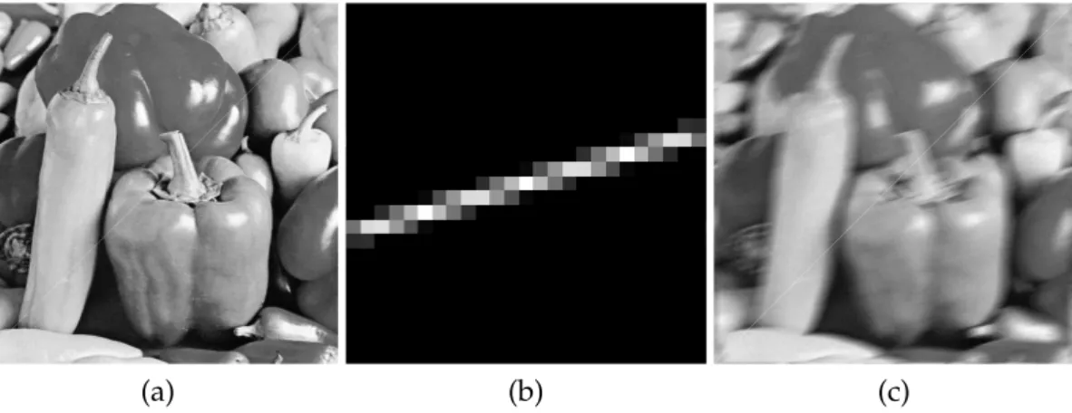
As we stated above, usually, the quality of the reconstruction can be improved by switching from the standard form to the general form. Before analyzing the theoretical properties of Tikhonov regularization in general form we want to give an example. We consider an image deblurring test case. We start with the peppers image in Figure 2.3(a) and we blur it using the motion PSF in Figure 2.3(b). In this way we are simulating the effect obtained when a picture is taken with a camera that is moving. We then add white Gaussian noise such that
δ= 0.02kbkand obtain the resulting blurred and noisy image in Figure 2.3(c) We refer to the
ratio
ξ = kηk
kbk, (2.13)
asnoise level. For the sake of simplicity in this example we are not considering the limited
FOV and we are assuming that the true image is periodic.
We then reconstruct with Tikhonov in standard and general form. For the general form we use as regularization operator the discretization of the two dimensional divergence operator. LetL1 be the finite difference discretization of the one dimensional derivative with periodic boundary conditions, i.e.,
L1= −1 1 −1 1 ... ... −1 1 1 −1 , we defineLas L=L1⊗I+I⊗L1, (2.14)
By choosing the optimalα, i.e., the one that minimizes the error, we obtain the reconstruction
in Figure 2.4. For the comparison of the two methods we consider the Relative Reconstruc-tion Error (RRE) defined as
RRE(x) =
x−x†
kx†k (2.15)
In Table 2.1 we show the RRE obtained with the different methods. We can see that the introduction of theL is able to increase the accuracy of the method. Moreover, from the
visual inspection of the reconstructions in Figure 2.4 we can see that Tikhonov in general form provides better restorations and in particular is able to lessen the so called ringing effect.
(a) (b) (c)
FIGURE2.3: Peppers test problem: (a) True image (512×512pixels), (b) motion
PSF (23×23pixels), (c) blurred and noisy image (ξ= 0.02).
(a) (b)
FIGURE 2.4: Peppers test problem reconstruction: (a) Tikhonov in standard form, (b) Tikhonov in general form. For both method the optimalαhas been
chosen.
We can now move to the theoretical analysis of (2.8). In particular, we want to see how it is possible to reduce the problem (2.8) in standard form (2.10).
IfLis invertible, then the minimization problem (2.8) becomes
min x=Lx AL−1x−bδ 2+αkxk2. (2.16)
Solving (2.16) leads toxαfrom which we can retrieve the solutionxαof (2.8) by multiplying
timesL−1:
xα =L−1xα.
When Lis not invertible, we follow [59]. LetA : X → Y and L : X → X be two linear operators between Hilbert spaces, theA−weighted pseudo-inverse ofLis
L†A= (I−(A(I −L†L))†A)L†. (2.17)
We define the vectors
x=Lx x(0) = (A(I−L†L))†bδ bδ=bδ−Ax(0)
and consider the problem
¯ xα = arg min x AL†Ax−bδ 2+αkxk2. (2.18)
2.2. Tikhonov Regularization 15
The solutionxαof (2.10) is obtained from the solutionxαof (2.18) by xα =L†Axα+x(0).
2.2.2 Iterated Tikhonov
In order to furtherly improve the quality of the solution provided by Tikhonov regulariza-tion, it is possible to use a refinement technique and formulate an iterative algorithm. The general idea behind refinement techniques is the following. Given the approximationxk
ofx†. Call
ek=x†−xk,
the approximation error ofxk, if we had access toekwe could easily obtainx†formxk, since x†=xk+ek.
We can computeekfrom the so callederror equation
Aek =A
x†−xk
=Ax†−Axk=b−Axk.
However, the computation of ek is not trivial. We have to consider that A is severely
ill-conditioned and that we do not knowb, but onlybδ. In other words we only have access to
the system
Aek≈rk=bδ−Axk.
Therefore, lettinghkbe an approximation ofek, we can refinexkby xk+1 =xk+hk.
We still have to resort to regularization methods to obtain a good approximation ofek, i.e., hk. We then use Tikhonov regularization in standard form to compute this approximation
hk= arg min
h kAh−rkk
2+α
khk2.
Summarizing we have
Algorithm 2.1(Iterated Tikhonov (IT)). Consider the linear system(2.3). Letx0be an initial guess forx†and letα >0be a constant.
for k= 1,2, . . .
rk=bδ−Axk
xk+1 =xk+ AtA+αI−1Atrk end
In Algorithm 2.1 the parameterα is chosen once and for all. The main issue with this
ap-proach is that the choice ofαis, again, crucial and may be difficult.
A more stable algorithm is obtained when the parameter α is changed at each iteration.
conditions. A sufficient condition is that
∞ X k=0
α−k1=∞, ∀k αk>0.
We can formulate then the following
Algorithm 2.2(Nonstationary Iterated Tikhonov (ITN S)). Consider the linear system(2.3). Let x0be an initial guess forx†and let{αk}kbe a sequence such that∀k αk >0andP∞k=0α−k1 =∞.
for k= 1,2, . . . rk =bδ−Axk xk+1=xk+ AtA+αkI −1 Atrk end
The convergence of both algorithm is assured by
Theorem 2.2([25]). Consider the linear system(2.3). Let{αk}kbe a sequence such that∀k αk >0
andP∞k=0α−k1=∞. Then the iterates generated by ITN Sconverges to the solution of (2.3)which is
nearest tox0. In particular, ifx0 =0, thenxk→A†bδask→ ∞.
The regularization inside both IT and ITN S is obtained by stopping the iteration before
con-vergence. In particular we can still apply the discrepancy principle, but in this case we use it as a stopping criterion, i.e., we continue the iterations until we reach the first iterationk∗
such that
krk∗k ≥τ δ and krkk< τ δ for k= 0,1, . . . , k∗−1, (2.19)
withτ >1.
The choice of the parameterαk is very important. A possible and popular solution is the
geometric sequence
αk=α0qk, (2.20)
whereα0 >0and0< q <1. Note that this sequence satisfies the hypothesis of Theorem 2.2. This choice is studied in [25,79].
We would like to stress that for both algorithms we have used the standard form of Tikhonov regularization, i.e., we have setL = I. We will see in Chapter 4 how to analyze the case of
17
Chapter 3
Constrained Tikhonov Minimization
As we said above, due to the fact that many singular values of the matrixA cluster at the
origin, the least-squares problem (2.3) may be numerically rank-deficient. Therefore, it is generally beneficial to impose constraints on the computed solution that the desired solution
x†is known to satisfy.
For instance, in image restoration problems the entries of the vectorx†represent pixel values
of the image. Pixel values are nonnegative and, therefore, it is generally meaningful to solve the constraint minimization problem
x+α = arg min
x≥0
Ax−bδ2+αkxk2 (3.1)
instead of (2.10). Herex ≥ 0is intended component-wise. In this chapter we are going to consider only Tikhonov regularization in standard form. A closed form of the solutionx+α
generally is not available.
LetΩdenote the nonnegative cone, i.e.,
Ω ={x∈Rn: (x)
i ≥0 1≤i≤n}, (3.2)
and letPΩ be the orthogonal projector fromRntoΩ. Thus, we determinePΩ(z)forz ∈ Rn by setting all negative entries ofzto zero. An approximation ofx+α is furnished by
xΩα =PΩ(xα) =PΩ
AtA+αI−1Atbδ. (3.3)
When x† ≥ 0, the vectorxΩα generally is a better approximation of x† thanxα. However,
typicallyx+α is a much more accurate approximation ofx†thanxΩα.
We want now to discuss the solution of the constrained Tikhonov regularization problem (3.1) by the modulus-based iterative method described in [122]. In [122] is discussed the application of this kind of method to the solution of nonnegative constrained least-squares (NNLS) problems, min x≥0 Ax−bδ (3.4)
with a matrix A ∈ Rm×n that is either well-conditioned or ill-conditioned. Since we are
considering the case in which the singular values ofA cluster at the origin we are able to
determine accurate approximate solutions of (3.1) in a Krylov subspace of, generally, fairly small dimension. This observation reduces the computational effort considerably.
We also consider the situation whenAis a BCCB matrix. Modulus-based iterative methods
for the NNLS problem (3.4) with a matrix with this type of structure can be solved efficiently by application of FFT.
We first review results about modulus-based iterative methods discussed in [7,57,76,122]. We then apply a modulus-based iterative method to the solution of large-scale constrained Tikhonov regularization problems (3.1). These problems are reduced to small size by a Krylov subspace method. This reduction lessens the computational effort required for the solution of the constrained Tikhonov regularization problem considerably.
We now give some comments on related work on the computation of nonnegative approx-imate solutions of problem (3.4) with a large matrixAwhose singular values cluster at the
origin. The importance of being able to solve this kind of problem has spurred the develop-ment of a variety of methods. In [102] is described a curtailed steepest descent method that determines nonnegative solutions. Active set methods based on Tikhonov regularization are developed in [98,101] and barrier methods for Tikhonov regularization are discussed in [35, 99,115]. A discussion of many optimization methods, including active set and barrier meth-ods, is provided in [106]. In our experience, it is beneficial to use methods that exploit special properties or structure of the matrixA. The fact that the matrixAcan be approximated well
by a matrix of low rank makes our Krylov subspace modulus-based method competitive with available Krylov subspace methods, because it only requires the computation of one Krylov subspace of modest dimension. This subspace then is used repeatedly. WhenAis a
BCCB matrix, fast solution methods are based on the fact that matrix-vector products withA
and the (pseudo-)inverse ofAcan be computed in onlyO(nlogn)arithmetic floating point operations (flops) with the aid of the FFT.
This chapter is organized as follows: Section 3.1 reviews results about modulus-based iter-ative methods discussed in [7, 57,76, 122]. We apply a modulus-based iterative method to the solution of large-scale constrained Tikhonov regularization problem (3.1). These prob-lems are reduced to small size by a Krylov subspace method. This reduction lessens the computational effort required for the solution of the constrained Tikhonov regularization problem considerably. In Section 3.3 we briefly discuss the Golub-Kahan bidiagonalization technique. Section 3.4 describes our Krylov subspace-based method for the solution of (3.1) and Section 3.5 contains a few computed examples. The latter section also illustrates how the BCCB structure of the matrixAcan be exploited.
3.1
Reformulation of the problem
This section summarizes results discussed in [57,76,122] of interest for the solution methods of the present chapter. Other recent discussions on modulus-based iterative methods can be found in [7,10] and references therein.
We reduce the constrained least-squares problem (3.4) to a linear complementarity problem, which we will solve by a modulus-based iterative method. The following result can be found in [42, Page 5, Definition 3.3.1 and Theorem 3.3.7]. It is also shown in [122, Theorem 2.1]. Theorem 3.1. LetMbe a symmetric positive semidefinite matrix. Then the nonnegative constrained quadratic programming problem,
min x≥0 1 2x tMx+ctx,
3.2. Modulus Method 19
denoted by NNQP(M, c), is equivalent to the linear complementarity problem,
x≥0, Mx+c≥0, and xt(Mx+c) = 0,
denoted by LCP(M,c).
The results below, shown in [57,76,122], are consequences of the above theorem.
Corollary 3.2. LetM ∈Rn×nbe symmetric and positive definite and letc∈Rn. Then the problems
NNQP(M,c) and LCP(M,c) have the same unique solution.
Corollary 3.3. The NNLS problem(3.4)is equivalent to LCP(AtA,−Atb),
x≥0, r=AtAx−Atb≥0, and xtr= 0.
It has a unique solution whenAis of full column rank.
Theorem 3.4. LetDbe a positive definite diagonal matrix and define fory= [y1, y2, . . . , yn]t∈Rn
the vector|y|= [|y1|,|y2|, . . . ,|yn|]t∈Rn.
(i) If(x,r)is a solution of LCP(AtA,−Atb), theny= (x−D−1r)/2satisfies
D+AtAy= D−AtA|y|+Atb. (3.5)
(ii) Ifysatisfies(3.5), then
x=|y|+y and r=D(|y| −y)
is a solution of LCP(AtA,−Atb).
Proof. The results can be shown using [7, Theorem 2.1].
From here on we will assume that the matrix Ahas full column rank. This requirement is
satisfied by the matrixA˜used in the following; see(3.16).
3.2
Modulus Method
Theorem 3.4, and in particular equation (3.5), suggest the fixed-point iteration
(D+AtA)yk+1 = (D−AtA)|yk|+Atb, (3.6)
which is the basis for the following algorithm.
Algorithm 3.1(Modulus Method (MM)). Lety0∈Rnbe an initial approximate solution of (3.5) and letDbe a positive definite diagonal matrix.
x0=y0+|y0|
for k= 0,1,2, . . .
yk+1 = (D+AtA)−1 (D−AtA)|yk|+Atb xk+1 =yk+1+|yk+1|
end
This algorithm is a special case of the modulus-based matrix splitting iterative methods pro-posed in [7]. Its convergence was investigated in [122] based on the analysis for HSS methods [9]. The case of interest to us is whenD=µInwithµ >0. This iterative method is analyzed
in [57,76]. We discuss the convergence of the iteratesykfor completeness. Lety∗denote the
solution of (3.5) forD=µIn, Then
yk+1−y∗ = (µIn+AtA)−1(µIn−AtA)(|yk| − |y∗|) and we obtain kyk+1−y∗k ≤(µIn+AtA)−1(µIn−AtA)k|yk| − |y∗|k ≤(µIn+AtA)−1(µIn−AtA) kyk−y∗k.
The matrix(µIn+AtA)−1(µIn−AtA)is symmetric. Therefore, (µIn+AtA)−1(µIn−AtA) = max λj∈λ(AtA) µ−λj µ+λj , (3.7)
whereλ(AtA) denotes the spectrum of AtA. Since A is of full rank, λ
j > 0 for all j and,
therefore, µ−λj µ+λj <1 ∀j. Hence, (µIn+AtA)−1(µIn−AtA)<1,
which shows convergence of the iterations (3.6) forD = µInwith µ > 0. The rate of
con-vergence generally increases when (3.7) decreases. Replacingλ(AtA)in the right-hand side of (3.7) by its convex hull gives an optimization problem whose solution can be easily deter-mined, µ∗ = arg min µ∈R max µmin≤µ≤µmax µ−λ µ+λ =pλminλmax. (3.8)
Hereλmin andλmaxdenote the smallest and largest eigenvalues ofAtA, respectively. Thus, the relaxation parameterµ∗ gives a near-optimal rate of convergence.
3.3
Golub-Kahan bidiagonalization
Before formulating our algorithm, we are going to recall some basic facts on Golub-Kahan bidiagonalization.
Golub-Kahan bidiagonalization algorithm applied to the matrix C ∈ Rm×n produces the
following factorization
VtCU =B, (3.9)
whereV ∈Rm×mandU ∈Rn×nare orthogonal matrices andB ∈Rm×nis a bidiagonal
ma-trix. For the moment we follow [73, Section 10.4.1] and soBis going to be upper bidiagonal.
Assume, without loss of generality, thatm > n, we writeBas
B = α1 β1 . . . 0 0 α2 β2 . . . 0 ... ... ... ... ... ... 0 αn−1 βn−1 0 . . . 0 αn 0
3.3. Golub-Kahan bidiagonalization 21
It is possible to show that a factorization of the form (3.9) exists ifC is of full column rank
(see [73, Section 5.4.8]). Moreover, since C and B are orthogonally related, they have the
same singular values. From (3.9) it follows that
CU =V B and CtV =U Bt.
WritingV, U in terms of their columns
V = [v1|. . .|vm] U = [u1|. . .|un] yields to Cuj =αjvj+βj−1vj−1, Ctvj =αjuj+βjuj+1 (3.10) (3.11) for1≤j≤n, with the notationβ0v0 ≡0andβnun+1 ≡0. Define
rj =Auj−βj−1vj−1,
pj =Atvj−αjuj.
(3.12) (3.13) Combining (3.10), (3.12) and the orthonormality of the vectorsvjwe get
αj =± krjk,
vj =rj/αj, (αj 6= 0).
Similarly from (3.11), (3.13) we have
βj =± kpjk,
uj+1 =pj/βj, (βj 6= 0).
Using this relation we get the following
Algorithm 3.2(Golub-Kahan upper bidiagonalization). LetC ∈ Rm×nwith full column rank.
Letu0 ∈Rnbe a vector of unitary norm. The following procedure computes the factorization(3.9).
k= 0, p0=u0, β0 = 1, v0 =0 While βj 6= 0 uj+1=pj/βj k=k+ 1 rj =Cuj−βj−1vj−1 αj =krjk vj =rj/αj pj =Ctvj−αjuj βj =kpjk end
The above algorithm can be stopped afterℓsteps forC that are not of full column rank as
long asℓis small enough.
It can be shown that
span{u1, . . . ,uℓ}=Kℓ(CtC,u0) span{v1, . . . ,vℓ}=Kℓ(CCt, Cu0)
where byKℓ(C,y)we denote the Krylov subspace of dimensionℓrelated to the pair{C,y},
defined as
Kℓ(C,y) = span{y, Cy, . . . , Cℓ−1y}.
By applying Algorithm 3.2 toCtwe obtain the factorization VtCtU =B,
equivalently
UtCV =Bt, (3.14)
whereU, V are orthonormal matrices andBtis lower bidiagonal.
Algorithm 3.3(Golub-Kahan lower bidiagonalization). LetC ∈ Rm×nwith full column rank.
Letu0 ∈Rnbe a vector of unitary norm. The following procedure computes the factorization(3.14).
k= 0, p0=u0, β0 = 1, v0 =0 While βj 6= 0 uj+1=pj/βj k=k+ 1 rj =Ctuj−βj−1vj−1 αj =krjk vj =rj/αj pj =Cvj−αjuj βj =kpjk end
It then follows that
span{u1, . . . ,uℓ}=Kℓ(CCt,u0) span{v1, . . . ,vℓ}=Kℓ(CtC, Ctu0)
3.4
Krylov subspace methods for nonnegative Tikhonov
regular-ization
We now combine the MM algorithm described in Section 3.2 with the Golub-Kahan lower bidiagonalization in Section 3.3. We describe the application of the modulus-based iterative method to Tikhonov regularization with nonnegativity constraint (3.1). We discuss how the computational effort for large-scale problems can be reduced by using a Krylov subspace method with a fixed Krylov subspace. Finally, we comment on how to exploit the BCCB structure ofAin image deblurring applications.
Application ofℓ ≪ min{m, n} steps of Golub-Kahan lower bidiagonalization, i.e., of
Algo-rithm 3.3, toAwith initial vectoru0 =bδ/kbδkgives the decompositions
AVℓ =Uℓ+1Bℓ+1,ℓ, AtUℓ =VℓBℓ,ℓt , (3.15)
whereUℓ+1 = [u1,u2, . . . , uℓ+1] ∈Rm×(ℓ+1) andVℓ = [v1,v2, . . . ,vℓ]∈Rn×ℓhave
orthonor-mal columns, Uℓ ∈ Rm×ℓ is made up of the first ℓ columns of Uℓ+1, Bℓ+1,ℓ ∈ R(ℓ+1)×ℓ is
lower bidiagonal with positive diagonal and subdiagonal entries, andBℓ,ℓis the leadingℓ×ℓ
3.4. Krylov subspace methods for nonnegative Tikhonov regularization 23
We assume for now thatℓis chosen small enough so that the decompositions (3.15) with the
stated properties exist. As stated in the previous Section we note that the columns ofVℓspan
the Krylov subspaceKℓ(AtA, Atbδ).
We first rewrite the minimization problem (3.1)
min x≥0 Ax−bδ2+αkxk2 = min x≥0 A √ αIn x− bδ 0 2 = min x≥0 A˜x−b˜δ2, (3.16)
where we assume thatα > 0. Then the matrix A˜ ∈ R(m+n)×n is of full column rank and
the minimization problem (3.16) satisfies the conditions in Section 3.2. Therefore, the iterates determined by Algorithm 3.1 will converge.
When the matrixAis large and without exploitable structure, the computations with
Algo-rithm 3.1 withD = µInmay be expensive. In particular, factoring the matrix µIn+ ˜AtA˜in
order to solve the linear systems of equations with this matrix required by Algorithm 3.1 may be unattractive or infeasible. We are interested in trying to reduce the computational effort required for solving these linear systems of equations. One way to achieve this is to solve them by the conjugate gradient method. It is convenient to use the CGLS implementation [16]. This solution approach is discussed in [122] and also illustrated in Section 3.5.
We now describe an alternative way to reduce the computational effort. We first determine an initial reduction ofA to a small bidiagonal matrix with the aid of Golub-Kahan lower
bidiagonalization. The Krylov solution subspace generated by this reduction method then is reused for all linear systems of equations with the matrixµIn+ ˜AtA˜that have to be solved.
Substitutingx = Vℓy, y ∈ Rℓ, into (2.10) and determining an approximate solution by a
Galerkin method gives the equation
Vℓt(AtA+αIn)Vℓy=VℓtAtbδ,
which, with the aid of the decompositions (3.15), can be expressed as
(Bℓt+1,ℓBℓ+1,ℓ+αIℓ)y=
e
1
Atbδ. (3.17)
Here and below
e
jdenotes thejth column of an identity matrix of appropriate order. There-duced Tikhonov equations (3.17) are the normal equations associated with the least-squares problem min y∈Rℓ B√ℓ+1,ℓ αIℓ y−√α
e
ℓ+2Atbδ . (3.18)We solve the latter instead of (3.17) fory = yα for reasons of numerical stability. For each
fixedα > 0the least-squares problem (3.18) can be solved in onlyO(ℓ)arithmetic floating-point operations [60] for details on the solution of least-squares problems of the form (3.18). We turn to the determination ofα > 0by the discrepancy principle. Substitutingxα =Vℓy
into (2.12) and using (3.15) gives the reduced problem
whereysolves (3.18).
Proposition 3.5. Introduce the function
φℓ(α) =kbδk2
e
t1(α−1Bℓ+1,ℓBℓt+1,ℓ+Iℓ+1)−2e
1. (3.20) Then the solutionα >0ofφℓ(α) =τ2δ2 (3.21)
determines a solutiony=yαof (3.18)that solves(3.19). The vectorxα,ℓ=Vℓyαsatisfies(2.12).
Proof. It follows from (3.15) that
Atbδ=AtUℓ
e
11kbδk=v1e
t1Bℓt+1,ℓe
1kbδk.Substituting this expression and the solution of (3.17) into the left-hand side of (3.19) gives
kBℓ+1,ℓ(Bℓt+1,ℓBℓ+1,ℓ+αIℓ)−1
e
1kAtbδk −e
1kbδk k2= kBℓ+1,ℓ(Bℓt+1,ℓBℓ+1,ℓ+αIℓ)−1Bℓt+1,ℓ
e
1−e
1k2kbδk2. (3.22) The identityBℓ+1,ℓ(Bℓt+1,ℓBℓ+1,ℓ+αIℓ)−1Bℓt+1,ℓ−Iℓ+1=−(α−1Bℓ+1,ℓBℓt+1,ℓ+Iℓ+1)−1
can be shown, e.g., by multiplication byBℓ+1,ℓBℓt+1,ℓ+αIℓ+1from the right-hand side. Sub-stitution into (3.22) gives
kBℓ+1,ℓyα−
e
1kbδk k2 =kbδk2e
1t(α−1Bℓ+1,ℓBℓt+1,ℓ+Iℓ+1)−2e
1,This shows (3.20). The fact that the vectorxµ,ℓsatisfies (2.12) follows from (3.15) and (3.19).
Proposition 3.6. Letφℓ(α)be defined by(3.20). Then the functionν →φℓ(1/ν)is strictly
decreas-ing and convex forν >0. Moreover,
lim
α→∞φℓ(α) =kb
δk2.
In particular, Newton’s method applied to the solution of the equationφℓ(1/ν) = τ2δ2 with initial
approximate solutionν0to the left of the solution converges monotonically and quadratically. Proof. The decrease, convexity, and limit follows from the representation
φℓ(1/ν) =kbδk2
e
t1(νBℓ+1,ℓBℓt+1,ℓ+Iℓ+1)−2e
1.Newton’s method converges monotonically and quadratically for decreasing convex func-tions when the initial iterate is smaller than the solution. The initial iterateν0 can be chosen to be zero with lim νց0φℓ(1/ν) =kb δk2, lim νց0 d dνφℓ(1/ν) =−2kb δk2kBt ℓ+1,ℓ
e
1k2.In actual computations it typically suffices to chooseℓ ≪ min{m, n}. We apply MM
3.4. Krylov subspace methods for nonnegative Tikhonov regularization 25
algorithm by
Tℓ,α=Bℓt+1,ℓBℓ+1,ℓ+αIℓ. (3.23)
Since the matrixBℓ+1,ℓis small, we can easily determine its largest singular valueσmax. Typ-ically, zero is a quite sharp lower bound for the smallest singular value. The largest eigen-value ofTℓ,αisσ2max+µand the smallest eigenvalue is bounded below by, and is generally close to,α. Hence, we will use the relaxation parameter
µ=p(σ2
max+α)α (3.24)
for the algorithm; cf. (3.8). This yields the following scheme.
Algorithm 3.4(Krylov subspace Modulus Method). Choose the number of Golub-Kahan lower bidiagonal steps,ℓ, and compute the decompositions(3.15). Determine a regularization parameter α
that satisfies(3.21)as described in Proposition 3.6. Compute the solutiony =yαof (3.18)and define
the initial approximate solutionx0 =PΩ(Vℓyα)of (3.1). Determine the largest singular value of the
matrixBℓ+1,ℓand define the relaxation parameter(3.24). LetTℓ,αbe given by(3.23).
ˆ
bδ=
e
1Atbδy0 =Vℓtx0 ˜
y0 =Vℓt|Vℓy0|
for k= 0,1,2, . . . until convergence yk+1= (µIℓ+Tℓ,α)−1(µIℓ−Tℓ,α)˜yk+ ˆbδ
˜
yk+1=Vℓt|Vℓyk+1|
end
x=Vℓy˜k+1+|Vℓy˜k+1|
The above algorithm computes the magnitude of every entry of an n-vector at each step.
Therefore, a transformation from theℓ-dimensional subspace, where the vectorsyk live, to Rnis required. Every step demands the solution of a linear system of equations of the form
(µIℓ+Tℓ,α)z=d
for some vectord. The solutionzcan be computed by solving a least-squares problem
anal-ogous to (3.18).
We remark that the Krylov subspaceK(AtA, Atbδ)is invariant under shifts ofAtAby a
mul-tiple of the identity, i.e.,
Kℓ(AtA, Atbδ) =Kℓ(AtA+µIn, Atbδ).
It follows that the shifted matrixµIℓ+Tℓ,αin Algorithm 3.4 corresponds to the shifted matrix
µIn+ AtA+αIn.
We described above how to determine the regularization parameterαby first reducing
equa-tion (2.12) to an equaequa-tion with a small matrix (3.19). When restoring images, we sometimes may impose periodic boundary conditions without affecting the quality of the computed restoration significantly. This yields a BCCB blurring matrixA ∈Rn×n, which can be
diago-nalized by the unitary Fourier matrixF defined in (2.7),
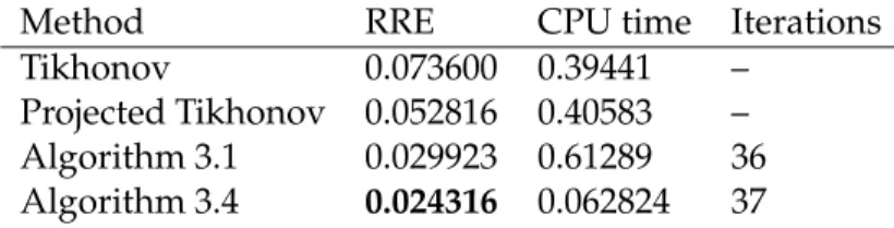
![Table 3.2 illustrates that, differently from the active set method [101], Algorithm 3.4 does not require more computational effort when the noise level is reduced](https://thumb-us.123doks.com/thumbv2/123dok_us/9467814.2821612/49.892.240.684.120.226/table-illustrates-differently-active-algorithm-require-computational-reduced.webp)

![Figure 8.1(a) reports an example of the behaviors of I(θ)/I(0) = K(θ, R)/K(0, R) versus θ over a range of [2 − 180 deg] for particles of different diameters d = 2R from d = 0.01 to 100 µm](https://thumb-us.123doks.com/thumbv2/123dok_us/9467814.2821612/149.892.134.753.129.347/figure-reports-example-behaviors-versus-particles-different-diameters.webp)
