Pricing Derivatives Securities
with Prior Information on
Long-Memory Volatility
Alejandro Islas Camargo* and Francisco Venegas Martínez**
Fecha de recepción: 18 de julio de 2001; fecha de aceptación: 8 de julio de 2002.
Abstract: This paper investigates the existence of long memory in the volatility of the Mexican stock market. We use a stochastic volatility (SV)
model to derive statistical test for changes in volatility. In this case, esti-mation is carried out through the Kalman filter (KF) and the improved
quasi-maximum likelihood (IQML). We also test for both persistence and
long memory by using a long-memory stochastic volatility (LMSV) model,
constructed by including an autoregressive fractionally integrated mov-ing average (ARFIMA) process in a stochastic volatility scheme. Under this
framework, we work up maximum likelihood spectral estimators and bootstraped confidence intervals. In the light of the empirical findings, we develop a Bayesian model for pricing derivative securities with prior information on long-memory volatility.
Keywords: contingent pricing, econometric modeling.
Resumen: Este trabajo investiga la existencia de memoria de largo plazo en la volatilidad del mercado bursátil mexicano. Se utiliza un modelo de volatilidad estocástica (SV) para derivar pruebas estadísticas de cambios en
la volatilidad. En este caso, la estimación de los parámetros se lleva a cabo a través del Filtro de Kalman (KF) y el método mejorado de cuasi máxima
verosimilitud (IQML). Asimismo, se prueba la persistencia y la memoria de
* ITAM, Departamento de Estadística, Río Hondo núm. 1, Col. Tizapán San Ángel, C.P.
01000, Del. Álvaro Obregón, México, D.F., e-mail: [email protected]. ** Oxford University.
We thank four anonymous referees of this journal for many valuable comments. In par-ticular, we are very grateful to one of them, for his very professional job in reviewing two previous drafts. In one of his numerous observations, he suggested that we split the manuscript into two articles: one including only the empirical issue, based on the frequentist approach, and the other one including the theoretical aspect, based on the Bayesian approach. This could be a good idea since we can have more room to deal with each issue separately. Moreover, two papers are always better than only one. However, we think that both parts have to remain together in order to provide a better understanding for pricing contingent claims with prior information on long-memory volatility. Alejandro Islas-Camargo wishes to thank the support from the Latin American and Iberian Institute at the University of New Mexico.
largo plazo utilizando un modelo de volatilidad estocástica de memoria de largo plazo (LMSV), el cual se construye incluyendo un proceso
auto-rregresivo y de promedios móviles integrado y fraccionario (ARFIMA) dentro
de un esquema de volatilidad estocástica. Bajo este marco, se trabaja con los estimadores espectrales de máxima verosimilitud y con intervalos de confianza generados con la técnica “bootstrap”. Con base en los resultados empíricos presentados, se desarrolla un modelo Bayesiano para valuar productos derivados cuando existe información a priori sobre volatilidad con memoria de largo plazo.
Palabras clave: valuación de productos, modelos econométricos.
1. Introduction
he consideration of prior information, before data is collected, when pricing contingent claims is not just a sophisticated extension but an essential issue to be taken into account for the theory and practice of derivatives. See, for instance, Korn and Wilmott (1996) and Jensen (2001). In contingent pricing, it is of particular interest to draw infer-ences about the volatility of the underlying asset on the basis of prior information.
The most common set-up of the continuous time stochastic volatil-ity model consists of a geometric Brownian motion correlated with a mean-reverting Orstein-Uhlenbeck process. This approach for pricing and hedging derivatives has been widely studied. See, for instance, Ball and Roma (1994), Heston (1993), Stein and Stein (1991), and Wiggins (1996). In particular, the stochastic volatility model allows us to reproduce in a more realistic way asset returns, specially in the presence of fat tails (Wilmott 1998), asymmetry in the distribution (Fou-que, Papanicolaou, and Sircar, 2000), and the smile effect (Hull and White, 1987). Despite this large body of theoretical advancement, the time continuous stochastic volatility model does not provide any eco-nomic intuition on the investor behavior. And, more importantly, there is a set of empirical regularities (or stylized facts) that are not repro-duced by the time continuous stochastic volatility model and still need to be explained. In particular, it is missing a satisfactory explanation of how investors, ranging from non corporate individual investors to large trading institution, choose a suitable distribution to model their expectations on the dynamics of volatility.
The temporal behavior of the stock market volatility has been, for the last decades, an issue of increasing interest. It is argued that, for
T
emerging stock markets, shocks to volatility persist for a very long time affecting significantly stock prices. The presence of long-memory volatility in asset returns has important implications for pricing con-tingent claims in emerging markets.
The growing economic importance of emerging stock markets char-acterized by singular institutional and regulatory frameworks provi-des an interesting environment to test for the existence of persistence
and long-memory components in the volatility.1 These markets
ex-hibit high (expected) returns as well as high volatility, and very little is known about the long-term effects of volatility. While the empirical literature has provided a considerable amount of research on infor-mation arrival and return volatility dynamics, it is missing a study on the persistence and long memory in the volatility in Latin American stock markets. This paper investigates the persistence and long memory components in the volatility of the Mexican stock market.
Data was obtained from the International Finance Corporation (IFC)
through Bloomberg, and spans from December 1988 to November 1998 yielding a sample size of 515 weekly observations.
Most of the empirical studies of long-memory processes have mainly concentrated on financial markets producing a large amount of re-search on the process specification in terms of the second moment (cf. Hurvich and Soulier, 2001). Ding, Granger and Engle (1993) proposed a model on the fractional moments, namely, the asymmetric power
ARCH model (A-PARCH). However, this model does not reproduce
appro-priately long-memory characteristics. More recently, Baille, Bollerslev and Mikkelsen (1996) presented a different approach to extend the
GARCH class to account for long memory, and developed the
fraction-ally integrated GARCH process (FIGARCH) which reproduces long
memory in volatility. Finally, Bollerslev and Mikkelsen (1996) extended
the model to the fractionally integrated exponential GARCH process
(FIEGARCH), which allows for nonsymmetrical shocks in the FIGARCH
scheme.
There is an alternative to the ARCH type modeling that allows the
variance to depend not only on past observations, but also on an underl-ying stochastic process driving the volatility, such as an autoregressive process. This model is called stochastic volatility or stochastic
vari-ance (SV) model. The SV model is also known in the literature as the
1 Regarding the institutional and regulatory framework and their effects on volatility for
mixture model. Clark (1973) introduced the SV model as a natural
way to model an unobservable variable. In his approach, the asset market is assumed to be in one of two states: a Walrasian equilibrium or a transitory equilibrium. As information arrives, heterogeneous agents reevaluate their desired portfolios and trade until they reach a new equilibrium. The market therefore goes through a sequence of equilibria. Clark (1973) models the variance by means of an i.i.d. log-normal process, finding a better fitting than alternative distributions such as the Poisson distribution. In a very stimulating paper Breidt, Crato and de Lima (1998) developed a model for the detection and estimation of long memory in the stochastic volatility framework
(henceforth LMSV). This model is constructed by including an
autoregressive fractionally integrated moving average (henceforth
ARFIMA) process in a stochastic volatility scheme SV.
Our plan for testing for persistence and long memory in the
vola-tility of the return rate of the Mexican IFC index has a number of
steps. First, we use stochastic volatility (SV) models, see for instance
Taylor (1986), to describe changes in volatility of the stock returns over time by treating volatility as an unobserved variable. This ap-proach is based on treating the logarithmic volatility as a linear sto-chastic process (more precisely, as an autoregressive model of order
1). The Kalman filter (KF) approach is then used to obtain smoothed
estimates and predictions of the underlying volatility. In this case, estimation is carried out through the improved quasi-maximum
like-lihood (IQML), suggested by Breidt and Carriquiry (1996). Second, we
test for the existence of a long-memory component in the SV by
apply-ing two traditional tests: 1) the modified rescaled range statistic, sug-gested by Lo (1991), and 2) the frequency domain analysis, proposed
by Geweke and Porter-Hudak (1983). Third, we use a LMSV model to
test for both persistence and long memory by working up maximum likelihood spectral estimators, as suggested by Breidt, Crato and De Lima (1998). Since our sample size (T = 515) is small compared with those used by Breidt, Crato and De Lima (1998), we used a bootstraped confidence interval for the parameters.
We find strong empirical evidence of long memory in the volatility of the Mexican stock market. It is shown that volatility of the Mexi-can stock market is fractionally integrated, so volatility does not re-turn to the previous mean after the occurrence of an exogenous shock. In section 3, we shall find that the long-memory parameter value is below a threshold value ½ in the statistical test. In the light of our
empirical findings, it is necessary to account for a satisfactory expla-nation of how investors incorporate in their expectations the long-term dynamics of volatility when making financial decisions. After all, agents should be able to catch up persistent volatility sooner o latter. In this paper, we develop a new Bayesian method to price de-rivative securities when there is prior information on long-memory volatility in terms of expected values of levels and rates, i.e., in terms of expectations on the potential level of volatility and on the rate at which volatility changes. In our proposal, investors are rational and use, efficiently, all prior information by maximizing an information measure on the set of all admissible prior distributions. After all, the core of finance theory (mathematical or empirical) is the study of the behavior of economic agents in an uncertain environment.
The paper is organized as follows. In the next section, we briefly
review the stochastic volatility (SV) model, the fractionally integrated
(ARFIMA) model, and the long-memory stochastic volatility (LMSV)
model. In section 3, we report our empirical findings on the basis of the SV, ARFIMA, and LMSV models. In section 4, we state the Bayesian
approach to prior information. In section 5, we develop a Bayesian model to price derivative securities with prior information on long-memory volatility. We also examine some asymptotic and polynomial approxi-mations and their implications in valuing contingent claims. Finally, in section 6, we present conclusions, acknowledge limitations, and make suggestions for further research.
2. Review of Econometric Modeling of Information Arrivals and Volatility Dynamics
Modeling volatility as a stochastic process is a complex issue. In the real world, volatility is not an observable variable and there is not a generally accepted stochastic volatility model. One of the most wide-spread set-up of the stochastic volatility model (see, for instance, Tay-lor, 1986), expresses the stochastic variance as:
(
/2)
, 1,2,..., ,exp
, h t T
yt=σtξt σt =ς t = (1)
where ht follows an AR(1) process:
. ) , 0 ( i.i.d. ~ , 2 1 η − +η η σ ϕ = h N ht t t t (2)
Here, ς is a constant, and ξt and ηt are assumed to be independent
processes. If the autoregressive parameter ϕ lies in (–1.1), then (2)
becomes a stationary process. If ξt and ηt are independent Gaussian
white noises with variances 1 and σ2
η, respectively, the scheme in (1)–
(2) is known as the log-normal SV model. One interpretation of the
log-volatility at time t, ht, is that it represents the random flow of new
information. The parameter ς plays the role of a constant scaling
fac-tor and can be thought of as the modal instantaneous volatility, ϕ is
the persistence in the volatility, and σ2
η stands for the volatility of the
log-volatility.
Although the above model is quite simple, it is capable of
repre-senting a wide range of behaviors for volatility. Like the ARCH models,
the SV model can give rise to high persistence in volatility. One of the
inconveniences of using SV models is that unlike the ARCH models, it
is difficult to write down the exact likelihood function. However, they do have other compensating useful statistical attractions, for instance, the model can be expressed in a linear state-space form. Some
ap-proaches for estimation in the SV model are: 1) the quasi-maximum
likelihood (QML) suggested by Nelson (1988), and Harvey, Ruiz and
Shephard (1994); 2) the hierarchical Bayesian approach proposed by Jacquier, Polson and Rossi (1994); and 3) the improved
quasi-maxi-mum likelihood (IQML) approach presented by Breidt and Carriquiry
(1996). It is worthwhile to remark that in the QML approach, the
non-linear stochastic volatility model is non-linearized and the resulting non-linear state-space model is treated as Gaussian. Nelson (1988), Harvey, Ruiz and Shephard (1994) employed approximate linear filtering methods to produce a quasi-maximum likelihood estimator, and pointed out that the accuracy of the normality approximation used in the filtering approach will worsen as the variance decreases. Notice that the
trans-formation from SV models into state-space models cannot be carried out
with observations close to zero. Indeed, the result from the transfor-mation becomes suspicious whenever applied to inliers.
Under the Bayesian framework, Jacquier, Polson and Rossi (1994) proposed a hierarchical method. The main characteristic of their method is its performance in parameter estimation and smoothing in
SV models by relying on the appropriate marginal posterior
distribu-tions. These authors use a Markov chain Monte Carlo (MCMC) method
and through sampling experiments showed that their estimates
per-formed well relative to the QML approach. On the other hand,
modified the log(y2
t) transformation to reduce the sensitivity of the
estimation procedure to inliers. Their proposal consists of applying a linear transformation to shifted values of the observations, where the shift is determined by the slope of the tangent line to the transforma-tion. In this regard, Breidt and Carriquiry (1996) carried out a sam-pling experiment similar to that of Jacquier, Polson and Rossi and showed that their approach significantly improved the performance
of the usual QML estimators. For most of the true parameter values in
the simulation exercise their improved QML (IQML) estimators
per-form as well as the Bayesian estimators in terms of bias. The IQML
estimators have, however, a higher root mean square error (RMSE) than
the Bayesian estimators.
2.1. The Quasi-Maximum Likelihood (QML) Estimator
Following Nelson (1988) and Harvey and Shephard (1993), after
trans-forming yt by taking logarithm of the square of yt, the following
state-space model is obtained:
log y2
t = logς2 + E[log(ξ2t)] + ht + εt (3)
= µ + ht + εt
where
ht = ϕht – 1 + ηt, t = 1,2,…,T. (4)
Here, the disturbance term satisfies εt = log(ξ2t) – E[log(ξ2t)]. In this
case, εt ~ i.i.d., and its statistical properties depend upon the
distribu-tion of ξt. If ξt ~i.i.d. N(0,1) it can be shown, according to the results in
Bartlett and Kendall (1946), that the mean and variance of log(ξ2
t) are
E[log(ξ2
t)] = –1.27 and σ2ε = π2/2, respectively. Also, it can be shown that
the skweness and the kurtosis are –1.5351 and 4, respectively. Nelson (1988) pointed out that under transformation (3), the model (1) – (2) is
easier to analyze. For instance, if the {εt} are non-Gaussian, the Kalman
filter (KF) can still be used to produce the best linear unbiased
estima-tor of ht given the logarithms of the squared previous returns.
Fur-thermore, the smoother provides the best linear unbiased estimator. The parameters can be estimated following the suggestion of Harvey, Ruiz and Shephard (1994) using the following quasi log-likelihood
, ) / ( 2 1 log 2 1 ) 2 log( 2 )} , ( log{ 1 2 1
∑
∑
= = ν − − π − = β T t t t T t t f f T y L (5)where β is the parameter to be estimated; νt is the one-step-ahead
prediction error; and ft is the corresponding mean squared error from
the Kalman filter. If (4) is a Gaussian state-space model, then (5) be-comes the exact likelihood; otherwise (5) is called the quasi-likelihood
and can be still used to provide a consistent estimator β^.
2.2. The Improved Quasi-Maximum Likelihood (IQML) Estimator
In transforming a stochastic volatility model into a state-space form, some problems arise when observations are close to zero since the transformation becomes suspicious whenever applied to inliers. Sev-eral remedies have been proposed to accommodate inliers. Breidt and Carriquiry (1996) modified the logarithmic transformation by evalu-ating not at the possibly zero measurement, but at a small enough shift, and then extrapolating linearly. Thus, in the stochastic volatil-ity context, Breidt and Carriquiry obtained the robustified
transfor-mation, x* t given by * * * * * 2 2 2 2 2 1 2 2 2 2 2 1 2 2 2 2 ˆ ) ˆ ( ) ˆ log( log ˆ ) ˆ ( ) ˆ log( t t t t t t t t t t t t t h x x y y x ε + + µ = σ σ δ σ σ δ + ξ − σ σ δ + ξ + σ = σ δ σ δ + − σ δ + = − − − − − (6) where
]
[
2 2 2 2 2 2 1 2 2 2) Elog( ˆ ) ( ˆ ) ˆ ( log *= ς + ξ +δσ σ− − σ +δσ σ− − δσ σ− µ t t t t t and .) ( log ˆ ) ˆ ( ) ˆ log( 2 2 2 2 2 2 1 2 2 * 2 *= ξ +δσ σ − ξ +δσ σ δσ σ −µ = ς ε − − − − t t t t t tHere, δ is some (small) constant, and σ^ 2 is the sample mean of y2
t.
Breidt and Carriquiry (1996) reported a value of δ = 0.005 as the
small-est value for which the excess kurtosis of {ε*
t} was near zero for a wide
range of parameter values. This value of δ also reduces substantially
the skewness of {ε*
{ε*
t} is no longer π2/2 when ξt is Gaussian and suggested that the
vari-ance of {ε*
t} be treated as a free parameter and estimated from the
data. This transformation reduces the sensitivity of the estimation
procedure to small values of yt. It is worthwhile to mention that Breidt
and Carriquiry’s (1996) IQML estimators have a better performance
than that of the QML estimators when dealing with small samples.
2.3. Persistence and long memory
Most of the recent empirical investigation of conditional variance models has suggested that stock markets volatility may display a type of long-range persistence. As we mentioned above, this type of
persis-tence cannot be appropriately modeled with traditional ARCH models.
The same limitation applies to SV models in their standard
formula-tion. A lot of observed time series, although satisfying the assumption of stationarity, seem to exhibit a dependence between distant obser-vations that, although small, is by no means negligible. This may be characterized as a tendency for large values to be followed by larger values of the same sign in such a way that the series seem to go through a succession of cycles, including long cycles whose length is compa-rable with the total sample size. This point of view has persuasively been argued by Mandelbrot (1969, 1972) in considering non-Gaussian distributions to explore the structure of serial dependence in economic time series. These findings show that market volatility displays
per-sistent features, but since both GARCH and the SV models in their
stan-dard formulation are short memory models, the only way to reproduce persistence is by approximating a unit root. Empirical evidence that this persistence in stock market volatility can be characterized as long memory has been presented in recent research by Breidt, Crato and de Lima (1998). These authors constructed a long memory stochastic
volatility model (LMSVM) by including an autoregressive fractionally
integrated moving average (ARFIMA) process in a stochastic volatility
scheme SV. In other words, ht is generated by a fractional noise:
. 1 0 ), , 0 ( NID ~ , ) 1 ( − =η η σ2 ≤ ≤ η d N h L d t t t (7)
Like the AR(1) model in (4), this process reduces to white noise at
How-ever, model (7) becomes stationary when d < ½. Thus, the transition from stationarity to non-stationarity proceeds in a different way to
that of the AR(1) model in (4). A negative value of d is quite legitimate.
Indeed, when ht is non-stationary, the first difference of ht provides a
stationary intermediate memory process when –½ # d # 0. More
gen-erally, ht can be modeled as an ARFIMA (p,d,q) defined as follows:
.) , 0 ( NID ~ , ) ( ) ( ) 1 ( 2 η σ η η Θ = Φ −L d L ht L t t N (8)
For a LMSV model, the QML estimation in the time domain becomes
less attractive because the state-space model can only be used by
ex-pressing ht as an AR or MA process and truncating at a suitably high
lag. As an alternative, a frequency domain solution has been provided by Breidt, Crato and De Lima (1998) in the following way. The spectral
density of (3), assuming that ht is generated by (8), is given by
, , 2 | ) ( | | 1 | 2 | ) ( | ) ( 2 2 2 2 2 π ≤ λ ≤ π − π σ + Φ − π β σ = λ ε λ − λ − λ − η β i d i i e e e f (9) where β=( ,σ2,σ2,ϕ1,ϕ2,...,ϕ ,θ1,θ2,...,θ )′ ε η p q
d . The frequency domain
quasi-likelihood function is )]}, ( / ) ( [ ) ( log{ 2 )} ( log{ [ /2] 1 1 λ + λ λ π = β β β = −
∑
f I f T L k T k T k (10)where [.] denotes the integer part, λk = 2πk/T, is the kth Fourier
fre-quency, and It(λk) is the kth normalized periodogram ordinate. By
maxi-mizing (10), Breidt, Crato, and De Lima (1998) find strong consistent
estimators of β.
3. Empirical Analysis of Information Arrivals and Stock Return Volatility Dynamics
Empirical evidence shows that while financial variables such as stock returns are serially uncorrelated over time, their squares are not. Therefore, in order to check for the appropriateness of long memory
component in the SV model, we will use a volatility proxy, namely, the
3.1. The IQML Estimates of SV Models
In Clark’s (1973) model, the asset market is assumed to be in one of two states: Walraisan equilibrium or a transitory equilibrium. Each time information arrives, the market reaches a new equilibrium. There-fore, according to Granger (1980), the stock price index (which involves heterogeneous dynamic relationships at the individual level that are then aggregated to form a time series) will be fractionally integrated and obey long memory. A long memory time series model is one
hav-ing spectrum of order λ–2d for small frequencies λ, d > 0. These models
have infinite variance for d $ ½, but finite variance for d < ½. Thus,
if different sets of heterogeneous agents reevaluate their desired port-folios and trade until they reach a new equilibrium, aggregating those individuals will produce fractional integration. One might expect that more restricted financial markets will generate homogeneous agents, while the least restricted financial markets will generate heteroge-neous agents. Therefore, we expect that the least restricted financial markets will be characterized by a larger degree of persistence and long memory component in volatility than restricted markets.
We apply now the IQML estimation method to Mexican stock
mar-ket index. The empirical analysis is carried out with the series of the first difference of the logarithms of the squared return rate. For con-venience, the rate of return has been corrected by their sample means.
Table 1 shows the IQML estimates of the parameters ς, ϕ, and σ2
η.
Val-ues of ϕ close to one indicate considerable persistence in log-volatility.
We observe that the estimate of the autoregressive parameter, ϕ, is
0.954, implying a high degree persistence of the log-volatility.
The IQML estimation of the SV model via the KF provides smoothed
and filter estimates of the variance component. The smoothed estima-tor, known simply as the smoother, is based on more information than
the filtered estimator, and so it will have a mean square error (MSE)
matrix which, in general, is smaller than that of the filtered estima-tor. Figure 1(a,b) shows the graph of the absolute value of the returns Table 1. IQML estimator of the SV model
Persistence Volatility Scaling factor ϕ of the log-volatility σ2η ς
0.954 0.063 0.787
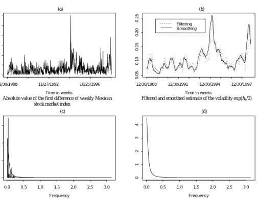
Time in weeks 0.0 0.10 0.20 0.30 12/30/1988 11/27/1992 10/25/1996 Time in weeks 0.05 0.10 0.15 0.20 0.25 12/30/1988 12/30/1991 12/30/1994 12/30/1997 Filtering Smoothing Frequency 0.0 0.5 1.0 1.5 2.0 2.5 3.0 0 2 4 6 Frequency 0.0 0.5 1.0 1.5 2.0 2.5 3.0 0 1 2 3 4 (a) (b) (c) (d)
Absolute value of the first difference of weekly Mexican stock market index
Filtered and smoothed estimate of the volatility exp(ht /2)
Periodogram of the estimate volatility Parametric estimates of the spectrum
Figure 1. Long-memory in the volatility on Mexico stock returns
and the resulting filtered and smoothed estimates of the volatility. These graphs show the expected feature of the filtered volatility lagging the smoothed volatility. Also, we notice that the smoothed estimate of the log-volatility for Mexico shows the behavior of a time series with a permanent component typical of a long memory time series. It is well known that the section of the spectrum of most interest in economic analysis is the low-frequency range, within which the long-run component is concentrated. Unfortunately, this range is the most difficult to deal with, and any trend in the series will give the zero frequency bands a large value. Finally, Figure 1(c,d) shows the perio-diogram and the parametric estimates of the spectrum of stock market volatility. As we can see, all spectra have a shape typical of an econo-mic variable (see Granger, 1966).
3.2. Testing for Long Memory in Volatility
Fractionally integrated models have received great attention because of their ability to produce a natural and flexible characterization of
the persistence process. In the general ARFIMA model given in (8), the
fractional differentiation operator (1 – L)d can be expressed as a
bi-nomial expansion. The process would be stationary and invertible if
–½ < d < ½. In case that d ? 0, the ARFIMA model displays a
substan-tial dependence between distant observations. Indeed, as time between
observations increases, the ARFIMA autocorrelations decline at a very
slow hyperbolic rate. In contrast, the ARMA autocorrelation declines at
an exponential rate.
Why fractional integration instead of testing for unit roots?
Frac-tional integration addresses a shortcoming that commonly used ARIMA
models have with modeling the degree and type of persistence in a
time series. ARIMA models have three parameters: p, d, and q. The
parameter corresponding to the number of lags involved in the auto-regressive portion of the time series is p. The parameter for the mov-ing average lags is q. Finally, d is a dichotomous variable indicatmov-ing whether the series is integrated or not. If the series is integrated, d takes a value 1. Otherwise, d equals 0, and the model is referred as an
ARMA model. ARFIMA models allow d to take any value, not just 0 or 1,
d is a real number. Instead of being forced into modeling data as ei-ther stationary, that is, I(0) or as integrated, that is I(1), we are more accurately model the dynamics of the series with fractional integra-tion, I(d), where d can still 0 or 1, but any fraction as well. If data are stationary, external shocks can have a short-term impact, but little long-term effects, as the data revert to the means of the series at an exponential rate. In contrast, integrated data do no decay, that is, do not return to the previous mean after an external shock has been felt.
ARIMA models do not account for the possibility that data can be mean
reverting while still exhibiting effects of shocks long since passed. By allowing d to take fractional values, we allow data to be mean revert-ing and to still have long memory in the process.
Geweke and Porter-Hudak (1983) propose a semi non-parametric
method for estimating d using the OLS regression based on the
periodogram. The significance of the fractional integration, d, is indi-cated by the standard t-statistics. One of the advantages to use this frequency domain regression method is that it allows the estimation
other statistic used to test for long memory is the modified rescaled
range statistic,2 suggested by Lo (1991). In this case, if only short
memory is presented, the modified rescaled range statistics,3 denoted
here by J^(T,q), converges to ½. If long memory is present, then J^(T,q)
converges to a value larger than ½. The first three columns of Table 2 report the results of the spectral regression tests. These three col-umns show the estimate of the parameter d with its corresponding p-value for the null hypothesis. This choice is made according to the suggestion in Geweke and Porter-Hundak’s (1983) work. Finally, no-tice that the estimates of the order of fractional integration are quite robust across the variation in u.
The values of the estimate of the parameter d are significantly different from zero. This indicates long memory for the stock market volatility of Mexico. The last two columns of Table 2 report the
esti-mates of J^(T,q), the modified rescaled range, and J^(T,q*), modified
rescaled range computed with Andrews’ (1991) data-dependent
for-mula. Values for both estimates, J^(T,q) and J^(T,q*) are significantly
different from ½, indicating long memory in the stock market volatil-ity. These findings suggest that volatility in the Mexican stock is frac-tionally integrated, which implies that volatility does not return to its previous mean after the occurrence of an external shock.
Table 2. Results of the Spectral tests
d^u = 0.50 d^u = 0.55 d^u = 0.60 J^(T,0) J^(T,q*)
0.433 0.571 0.303 0.660 0.634
(0.046) (0.004) (0.027) (0.000)
Results of the spectral tests and the R/S analysis: The integration parameter d is estimated with lower truncation at mL = [T0.17] and different upper truncations m
u = [Tu], u = 0.50, 0.55,
0.60. The modified Hurts statistics, J^(T,q), are estimated with q = 0, and q = q*. The latter is the value chosen by Andrew’s data-dependent formula. Unilateral test p–values for d and for the modified rescaled range statistic are displayed within parentheses.
2 The rescaled range statistic was first introduced by Hurst (1951) in studying long-term
storage capacity of reservoirs.
3 For details and explicit formulas of the modified rescaled range statistic, we direct the
3.3. Long-Memory Stochastic Volatility (LMSV) Model
We now test for long memory by using the long-memory stochastic
volatility (LMSV) model suggested by Breidt, Crato, and De Lima (1998).
This approach to testing for long memory provides a feasible frequency
domain likelihood estimator for the parameters in the LMSV model. In
this case, the returns yt are modeled as
yt = ht + εt
where εt ~ i.i.d. N(0, σ2ε). Here, εt and ht are supposed to be
indepen-dent, and ht follows an ARFIMA(1,d,0) process as defined in (8). The
spectral likelihood for the yt’s is formulated in equation (10). In this
case, assuming εt normally distributed, the resulting likelihood is
maximized with respect to d and ϕ. Table 3 reports the maximum
likelihood spectral estimators for σ2
η, d, and ϕ. The estimate of the
autoregressive parameter, ϕ, with a value 0.953, indicates persistence
in the log-volatility in the Mexican market stock. The estimate of the parameter d lies in 0 < d < ½, suggesting that the log-volatility has long-term persistence. Moreover, the autocorrelation of the log-vola-tility are positive and decay monotonically and hyperbolically to zero as the lag increases. The spectral density of the log-volatility is shown in Figure 1(d). The spectral density is concentrated at low
frequen-cies: fy(λ) is a decreasing function of λ and fy( )λ → ∞ as λ→0, and
fy(λ) is integrable. Hence, the spectrum as a whole has a shape typical
of an economic variable (see Granger, 1966).
Finally, it is important to point out that Breidt, Crato and De Lima (1998) reported that maximum likelihood estimation in the spectral domain perform well for relatively large samples (T = 4 096), while the Table 3. Spectral Likelihood Estimator
Persistence Volatility Fractional integration ϕ of the log-volatility σ2η parameter d
0.953 0.094 0.257
(0.089) (0.116) (0.631)
(0.762, 1.053) (0.001, 0.251) (0.179, 0.598)
Values in the table represent the maximum likelihood spectral estimator for σ2η, d, and ϕ
assuming εt to be normally distributed.
Standard deviation are given in parentheses. Bootstraped confident intervals are also provided.
performance for small samples (T = 1 024) may produce large outliers
in the estimation of ϕ, σ2
η, and d. Since our sample size (T = 515) is
small compared with those used by Breidt, Crato and De Lima (1998), we used a Bootstraped confidence interval for our parameter estimates. Indeed, Breidt et al. (1988, p. 339) present the finite sample proper-ties of the spectral likelihood estimator. In their simulation study of the finite sample properties of the spectral likelihood estimator they consider two different sample sizes (T = 1 024 and T = 4 096). Breidt et al. reported that maximum likelihood estimation in the spectral do-main perform well for relatively large samples (T = 4 096), while the performance for small samples (T = 1 024) may produce large outliers in the estimation of the parameters.
As a consequence of the empirical findings, it is important to de-velop a model for pricing and hedging derivative securities with prior information on volatility that account for information arrivals and volatility persistence. The model should provide a satisfactory expla-nation of how investors incorporate in their expectations the long-term behavior of volatility when making financial decisions. In the next two sections, we develop a Bayesian method to price and hedge derivative securities when there is prior information on long-memory volatility in terms of expected values of levels and rates. In our pro-posal, investors are rational and use, efficiently, all prior information by maximizing Jaynes’ information measure.
4. The Bayesian Approach to Prior Information
In the real world, volatility is neither constant nor directly observed. Hence, it is natural to think of volatility as a random variable with some initial knowledge coming from practical experience and under-standing. This is just the Bayesian way of thinking about prior infor-mation. Under this approach, prior information is described in terms of a probability distribution (subjective beliefs) of the potential values of volatility being true. In this regard, in Bayesian inference instead
of studying volatility, σ2 > 0, it is common to study precision, which is
defined as the inverse of the variance, h = σ–2; see, for instance, Leonard
and Hsu (1999), and Berger (1985). Thus, the lower the variance, the higher the precision. More precisely, from the Bayesian point of view,
we have a distribution, Ph, h > 0, describing prior information. We will
measure v, so that the Radon-Nykodim derivative provides a prior density, π(h): i.e., dPh/dν(h) = π(h) for all h > 0, so
{
∈}
=∫
π νA
h h A h h
P ( )d ( )
for all Borel sets A.
4.1. Maximum Entropy Priors
There are several well-known methods reported in the Bayesian lit-erature to construct densities that incorporate prior information by maximizing a criterion functional subject to a set of constraints in terms of expected values. Some of them are non-informative priors (Jeffreys, 1961), maximal data information priors (Zellner, 1977),
maxi-mum entropy priors (Jaynes 1968), minimaxi-mum cross-entropy priors4
(Kullback, 1956), reference priors (Good 1969, and Bernardo 1979), and controlled priors (Venegas-Martínez, De Alba, and Ordorica-Me-llado, 1999). We will specialize in this paper in Jaynes’ maximum entropy for pragmatic and theoretical reasons that will appear later.
If volatility is persistent, agents will learn in the long run about the likelihood of potential patterns of volatility. Let us suppose that there is information on long-memory volatility in terms of expected values. Specifically, suppose that information on long-memory preci-sion is given by , ,..., 2 , 1 , 0 , ) ( d ) ( ) (h h I{ 0} vh k N ak π h =γk =
∫
> (11)where the functions ak(h) are Lebesgue-measurable known functions
and all the constants γk are known. The function I{h > 0} stands for the
indicator function defined on {h|h > 0}. The maximum entropy prin-ciple states that among all densities satisfying the given information (constraints) we should choose the one that maximizes
. ) ( d ) ( )] ( ln[ )] ( [ 0
∫
> π π − = π h h h v h h H (12)4 Other model that uses this functional criterion in pricing derivative securities is that of
Avellaneda, Levy and Parás (1995), they assume that potential volatility values occur within a band, more precisely within an open interval.
We define a0(h) ; 1 and γ0 = 1 to ensure that the solution is indeed
a density. Hence, we are interested in finding π(h) that solves the
fol-lowing variational problem:
,) ( d ) ( )] ( ln[ )] ( [ Max 0
∫
> π π − = π h h h v h h H subject to C:∫
ak(h)π(h)I{h>0}dv(h)=γk, k=0,1,2,...,N. In the sequel, we will assume that the set of the constraints, C,forms a convex and compact set on π(h) in the topology of L2 ([0, ∞],
π(h) dν(h)). Since H[π(h)] is strictly concave in π(h), the solution exists
and is unique. In such a case, the necessary condition for π(h) to be a
maximum is also sufficient. By using standard necessary conditions derived from calculus of variations (see, for instance, Chiang, 1999), we found that λ = π
∑
= λ + N k k k h a e h 1 1 exp ( ) ) ( 0 (13)where λk, k = 0,1,2,…, N are the Lagrange multipliers associated with
the above variational problem. Such multipliers are to be determined from C.
4.2. Examples of Priors on Long-Memory Volatility
If market volatility is persistent, agents will learn in the long run about the likelihood of both the potential level of volatility and the rate at which volatility changes. Let us suppose that there is initial information on long-memory volatility in terms of expected values. More specifically, suppose that long-memory information on precision is given in terms of expected values of levels and rates. That is, prior knowledge is expressed as , / ) ( d ) ( 0 π =β α
∫
h> h h v h (14) and , ) ln( ) ( ) ( d ) ( ) ln( 0 π =ϕ α − β∫
h> h h v h (15)where α > 0, β > 0, ϕ(a) = dΓ(α)/dα, and Γ(.) is the Gamma function. Notice that for given expected values on levels and rates, equations
(14) and (15) become a nonlinear system in the variables α and β. It
can be easily shown that the Gamma distribution
, 0 and 0 , 0 , ) ( ) , | ( 1 > α> β> α Γ β = β α π h hα− αe−βh h (16)
solves the optimization problem. Another priors of interest could be: ; 0 and , 0 , 0 , ) ( , 1 1 > β > α > α Γ β = α β π hα+ αe−β h h h ; 0 and , 0 , 0 , ) ( 2 , 1 (1/2) > β > α > α Γ β = α β π hα+ αe−β h h h and ; 0 and , 0 , 0 , ) ( )} / 1 ln( exp{ , 1 log log(1/ ) > α> β> α Γ − β − β = α β π α e− h h h h
which stand, respectively, for prior distributions of σ2, σ, and log(σ2).
In any case, the best choice should reflect what has been learned from data. We will also study these possibilities in the rest of the paper. 5. The Bayesian Valuation Problem
Let us consider a Wiener process W(t), t > 0, defined on some fixed
filtered probability space (Ω, F, (Ft)t > 0, P), and European call option on
an underlying asset whose price S(t) is driven by a geometric Brown-ian motion accordingly to
dS(t) = rS(t)dt + h–1/2 S(t) dW(t),
that is, W(t), t > 0, is defined on a risk neutral probability measure P.
The option is issued at time t0 = 0 and matures at date T > 0 with
strike price X. Under the Bayesian framework, we have that the price
at time t0 = 0 of the contingent claim when there is information on
{
}
, ) ( d ) ( d ) ( ) ( ] ) 0 ( | 0 , ) ( E[max( E ) , | , , ); 0 ( , 0 ( 0 ( )| (0) ) ( h h s s f X s e S X T S e r T X S c h s X ST S rT rT ν π − = − = β α∫ ∫
> > − π − where{
( /2 ) ( ) ( /2 )}
. exp 2 ) ( 1/2[
]
) 0 ( | ) ( h T G s T h T s h s fST S − + π = and G(s) = ln[serT/S(0)].If we assume that the required conditions to apply Fubinis’ theo-rem are satisfied, then we can guarantee that integrals can be inter-changed and (17) becomes (most of the formulas and mathematical details can be found in Gradshteyn and Ryzhik, 1980)
∫
> α − β α − α Γ π β = X s rT s s J X S T e c [1 ( / )] ( | , )d ) ( 2 (18) where{
( /2 )[ ( ) ( /2 )]}
d ( ). exp ) , | ( 0 ) 2 / 1 ( 2∫
> β − − α ν + − = β α h h h e h h T s G T h s J (19)Notice now that (19) can be, in turn, rewritten as
{
−}
∫
>{
− −}
δ− ν = β α 0 1d ( ) ) / ( ) ( exp 2 / ) ( exp ) , | ( h A s h B h h h T s G s J where . 0 2 1 and , 8 / , 0 2 2 ) ( ) ( = 2 + βT> B=T δ= +α> T s G s AIn this case, the integral in (19) satisfies
{
( /2 )[ ( ) ( /2 )]}
d ( ) 2( / ( ))(
2 ( ))
exp /2 0 1 h B A s K BAs h h T s G T h h δ δ > − δ ν = + −∫
(20)where Kδ(x), x=2 BA(s), is the modified Bessel function of order δ
which is the solution of the second-order ordinary differential equa-tion (see, for instance, Redheffer 1991).
. 0 1 1 2 2 = + δ − ′ + ′′ y x y x y
We also have that Kδ(x) is always positive and Kδ(x)→0 as x→∞.
Equation (20) is of noticeable importance, it says that all information on long-memory volatility provided by the prior distribution and the relevant information on the process driving the dynamics of the
un-derlying asset are now contained in Kδ(x).
5.1. Constant Elasticity Instantaneous Variance
Let us assume that the underlying asset evolves according to
dS(t) = rS(t)dt + h–1/2S(t)b/2dW(t),
where the elasticity of stock returns variance with respect to the price equals b – 2. If b = 2 the elasticity is zero and asset prices are lognor-mally distributed. In this section, we are concerned with the case b < 2. In this case,
(
2 ( ))
) ) ( ( ) ( 1 2 1/(4 2 ) [ ()] ) 0 ( | ) ( D BAs e I h BAs h s f b b hB As S T S = δ − − − + δ where b b rT A s Ds e DS B b r D b = − = − = − − = δ 1/(2 ,) 2 /(2 ,) [ (0) ]2 , ( ) ( )2and Iδ(x), x=2h BA(s), is the modified Bessel function of the first
kind of order δ. If we assume that prior distribution is described by a
gamma density, then
∫
> − − α − β α − α Γ π δ β = X s b b rT s s Z s BA X s T e D c ( )[ ( ) ] ( | , )d ) ( 2 ) 2 4 /( 1 2 1 where{
}
(
)
∫
> δ α − β+ + = β α 0 exp [ ( )] 2 ( ) d ( ,) ) , | ( h h h B A s I h BA s ? h s Zwhich is related with the non central chi-square density function. Moreover,
(
)
. ) 1 ( ) 1 ( )] ( [ ) ( 2 0 2 2∑
∞ = δ + + δ δ = Γ + Γδ+ + k k k k k s BA h s BA h I Therefore,{
}
. ) 1 ( ) 1 ( ) 1 2 ( )] ( [ )] ( [ )] ( [ ) ( d )] ( [ exp ) 1 ( ) 1 ( )] ( [ ) , | ( 0 2 0 2 0 2 2∑
∫
∑
∞ = α δ > + δ + α ∞ = δ + + δ + + δ Γ + Γ + + δ + α Γ + + β = + + β − + + δ Γ + Γ = β α k k h k k k k k k k s BA s A B s BA h ? s A B h h k k s BA h s Zwhich can be used for large enough k. 5.2. Asymptotic Approximations
In this section we find an approximate formula for pricing vanilla contingent claims. In order to use asymptotic approximations, we have to make some assumption on the strike price, X. Note first that if the strike price X is large, then x is large. In such a case, we have
, 8 4 1 1 2 ) ( ˆ ) ( 2 − − δ π = ≈ − δ δ x K x x e x K x
which in practice performs well. In this case, we have as an estimate price ) , | , , ); 0 ( ( ) , | , , ); 0 ( ( ) 0 ( ˆ =S L1 S T X r α β −e− XL2 S T X r α β c rT (21) where
{
[ (1/2) ()]}
( / ()) ˆ(
2 ( ))
d , exp 2 ) 0 ( ) , | , , ); 0 ( ( /2 1 r G s T As K BAs s T S r X T S L X δ δ ∞ α + − π β = β α∫
and{
(1/2) ( )}
( / ( )) ˆ(
2 ( ))
d . exp ) / 1 ( 2 ) , | , , ); 0 ( ( /2 2 s G s T A s K BAs s T r X T S L X δ δ ∞ α − π β = β α∫
The integrals L1 and L2 can be approximated with simple
proce-dures in Mathematica o MATLAB by using a large enough upper limit
in the integral.5 Figure 2 shows the values c^ as a function of α and β
with S(0) = 42.00, X = 41.00, r = 0.11 and T = 0.25.
5.3. Polynomial Approximations
Polynomial approximations can be done only for numerical values of the parameters. We apply the Frobenius’ method to obtain an ap-proximate polynomial of finite order. Let us consider the particular
case α = 1/2, i.e., δ = 1, in equation (19). The following polynomial
Figure 2. Values of c^ as a function of α and β
5 The upper limit of the integral L1 and L2 are such that when a larger upper limit is used,
approximation is based on Frobenius’ method of convergent power-series expansion: , 2 0 , 2 ) ( 2 ln 1 ) ( 6 0 2 1 1 < ≤ ε + + ≈
∑
= x x a x I x x x x K k k k (22)where the coefficients satisfy:
, 00004686 . 0 , 0110404 . 0 , 01919402 . 0 , 18156897 . 0 , 67278579 . 0 , 15443144 . 0 , 000000000 . 1 6 5 4 3 2 1 0 − = − = − = − = − = = = a a a a a a a and , 4 15 0 , 15 4 ) ( 6 0 2 1 < ≤ ε + ≈
∑
= x x b x x I k k k where , 00032411 . 0 , 00301532 . 0 , 02658733 . 0 , 15084934 . 0 , 51498869 . 0 , 87890594 . 0 , 500000000 . 0 6 5 4 3 2 1 0 = = = = = = = b b b b b b bwith ε < 8 × 10⁻⁹. The complementary polynomial is given by
, 2 , 2 ) ( 2 ln 1 ) ( 6 0 2 1 1 + ρ > + ≈
∑
= − x x e x I x e x x K k k k x (23) where , 00068245 . 0 , 00325614 . 0 , 00780353 . 0 , 01504268 . 0 , 03655620 . 0 , 23498619 . 0 , 25331414 . 1 6 5 4 3 2 1 0 − = = − = = − = = = e e e e e e e and , 4 15 , 15 4 ) ( 8 0 1 > ρ + ≈∑
= − x x g x x I k k k where, 00420059 . 0 , 01787654 . 0 , 02895312 . 0 , 02282967 . 0 , 01031555 . 0 , 00163801 . 0 , 00362018 . 0 , 03988024 . 0 , 39894228 . 0 8 7 6 5 4 3 2 1 0 − = = − = = − = = − = − = = g g g g g g g g g
with ρ < 2.2 × 10⁻⁷. It is important to point out that K
δ(x) and Iδ(x) are linearly independent modified Bessel functions, and hence, they de-termine a unique solution of Bessel differential equation. If we denote by K(ε)(x)
δ the polynomial approximation in (22) and (23), we get from
(21) and (20) the following call option price:
. ) , 5 . 0 | , , ); 0 ( ( ) , 5 . 0 | , , ); 0 ( ( ) 0 ( ˆ () 2 ) ( 1 ) (ε =S Lε S T X r α= β −e− XLε S T X r α= β c rT As before, integrals ( ) 1ε L and ( ) 2ε
L can be approximated by using
simple procedures in Mathematica or MATLAB. Figure 3 shows the
values c as a function of ˆ(ε) β with α = 0.5, S(0) = 42.00, X = 41.00,
r = 0.11 and T = 0.25.
In the Mexican case, there is not an exchange for trading stock options and the over-the-counter market on stock options is an incipi-ent market, so the data is poor in both quantity and quality. Hence, it Figure 3. Values of cˆ(ε) as a function of β
c^( )ε 3.5 3 2.5 2 1 2 3 4 β
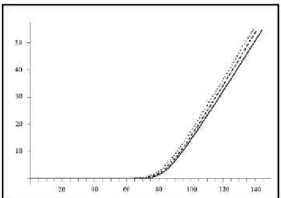
is impossible to carry out a reliable empirical analysis to compare market prices with our theoretical prices. However, we carry out an interesting numerical experiment. In this experiment, we compare our pricing approach with two other prices from models available in the literature. In Figure 4, the case of the classical Black and Scholes’ (1973) price, as a function of the strike price, is considered as a
bench-mark with parameter values S0 = 100, T = ½, r = 0.05, σ = 0.2, and is
represented by the continuous line. The Korn and Wilmott’s (1996) price with subjective beliefs on future behavior of stock prices is
rep-resented by the dashed line.6 Finally, the doted line shows our price c^
with prior information on long-memory volatility consistent with the
parameter values β = 17 and α = 0.5.7 Intuitively, and as it should be
expected, prices with initial beliefs on long-memory volatility on lev-els and rates take into account more information than prices with only initial beliefs on future levels of stock prices. Therefore, option prices with prior information on long-memory volatility should be higher than option prices with only prior information on future prices. As expected, Black and Scholes prices are smaller than option prices with prior information.
Figure 4. Option Values as a Function of the Strike Price
6 The parameter values in the Korn and Wilmott’s (1996) work are µ = 0.1, α = 0.33, β =
3.33, and γ = 0.1.
7 We examined, in this experiment, about 800 different combinations of the parameter
6. Summary and Conclusions
We have investigated the persistence and long-memory characteris-tics of volatility in the Mexican market stock. There are several methods to test for long memory, ranging from fully parametric to non-para-metric approaches. We have used both to investigate the existence of long memory in the volatility of the Mexican stock market and show that the results are consistent between them. Moreover, we have seen that autoregressive fractionally integrated moving average processes al-low a more flexible modeling of the al-low-frequency behavior of returns with important implications for the measurement of long-term vola-tility.
In the light of our empirical findings, we have developed, in a richer stochastic environment, a Bayesian procedure to price and hedge derivative securities when there is prior information on long-memory volatility. Specifically, this information was expressed in terms of ex-pectations on the potential level of volatility and on the rate at which volatility changes. It is important to point out that our theoretical frame-work led to the modified Bessel functions. By using asymptotic and polynomial approximations of these functions, we have provided sev-eral formulas for pricing contingent claims.
The broad message of this paper, although only demonstrated for the Mexican case, is that shocks to volatility persist for a very long time affecting significantly stock prices. Hence, hedging strategies of a long position should be taking into account the long-memory effects in a short position in a call option. This will certainly provide a more effective protection against negative effects of long-range persistence in volatility.
Needless to say, the model is obviously simple and could be ex-tended in several ways. First, further research should be undertaken to deal with the case of American options, which are more popular in derivatives exchanges and over-the-counter markets throughout the world. Second, additional investigation is needed to include in the Bayesian pricing formula the probabilistic behavior of the interest rate; for instance, we might contemplate a term structure driven by a Markovian diffusion process. Third, one of the limitations of our pro-posal is that there are no transaction costs and more should be done in this regard to obtain more realistic and representative pricing for-mulas. These extensions will lead to more complex market environ-ments and results will certainly be richer.
References
Andrews, D. (1991), “Heteroskedasticity and Autocorrelation Consis-tent Covariance Matrix Estimation, Econometric, No. 59, pp. 817-858.
Avellaneda, M., A. Levy and A. Parás (1995), “Pricing and Hedging Derivative Securities in Markets with Uncertain Volatilities”, Appl. Math. Finance, Vol. 2, pp. 73-88.
Avellaneda, M., C. Friedman, R. Holmes and D. Samperi (1996), “Cali-brating Volatility Surfaces Relative-Entropy Minimization”, Appl. Math. Finance, Vol. 4, No. 1, pp. 37-64.
Ballie, R.T., T. Bollerslev and H.O. Mikkelsen (1996), “Fractionally Integrated Generalized Autoregressive Conditional Heteroskedas-ticity”, Journal of Econometrics, No. 74, pp. 3-30.
Ball, C. and A. Roma (1994), “Stochastic Volatility Option Prices”, Jour-nal Financial and Quantitative AJour-nalysis, Vol. 24, No. 4, pp. 589-607. Bartlett, M.S. and D.G. Kendall (1946), “The Statistical Analysis of Variance-Heterogeneity and The Logarithmic Transformation”, Supplement to the Journal of the Royal Statistical Society, Vol. VIII, pp. 128-133.
Berger, J.O. (1985), Statistical Decision Theory and Bayesian Analy-sis, New York, Springer-Verlag.
Bernardo, J.M. (1979), “Reference Posterior Distributions for Baye-sian Inference”, Journal of the Royal Statistical Society, vol. B41, pp. 113-147.
Black, F., and M. Scholes (1973), “The Pricing of Options and Corpo-rate Liabilities”, Journal of Political Economy, Vol. 81, pp. 637-659. Bollerslev, T. and H.O. Mikkelsen (1996), “Modeling and Pricing Long-Memory in Stock Market Volatility”, Journal of Econometrics, Vol. 73, pp. 151-184.
Breidt, F.J. and A.L. Carriquiry (1996), “Improved quasi-Maximum Likelihood Estimation for Stochastic Volatility Models”, in Jack C. Lee, Wesley O. Johnson and Arnold Zellner (eds.), Modeling and Prediction: Honoring Seymour Geisser, New York, Springer-Verlag, pp. 228-247.
Breidt, F.J., N. Crato and P.J.F. de Lima (1998), “The Detection and Estimation of Long Memory in Stochastic Volatility”, Journal of Econometrics, Vol. 83, pp. 325-348.
Chiang, C.A. (1999), Elements of Dynamic Optimization, Waveland Press.
Clark, P.K. (1973), “A Subordinated Stochastic Process Model with Finite Variances for Speculative Prices”, Econometrica, vol. 41, pp. 135-156.
Clewlow and Hodges (1997), “Optimal Delta-Hedging under Transac-tion Costs”, Journal of Economic Dynamics and Control, núm. 21, pp. 1553-1376.
Cyert, R.M. and M. H. Degroot (1987), Bayesian Analysis and Uncer-tainty in Economic Theory, Rowman & Littlefield Probability and Statistics Series, Rowman & Littlefield.
Davis, M.H.A., V.G. Panas and T. Zariphopoulou (1993), “European Option Pricing with Transaction Costs”, SIAM Journal of Control and Optimization, Vol. 31, No. 1, pp. 470-493.
De Lima, P.J.F. and N. Crato (1993), “Long-Range Dependence in the Conditional Variance of Stock Returns”, Joint Statistical Meetings, San Francisco, Proceedings of the Business and Economic Statistics Section, August.
Ding, Z., C. Granger and R.F. Engle (1993), “A Long Memory Property of Stock Market Returns and a New Model”, Journal of Empirical Finance, vol. 1, pp. 83-106.
Dorfman, J.H. (1997), Bayesian Economics through Numerical Meth-ods: A Guide to Econometrics and Decision-Making with Prior In-formation, Springer Verlag.
Engle, R.F. (1982), “Autoregressive Conditional Heteroskedasticity with Estimates of the Variance of the United Kingdom Inflation”, Econo-metrica, Vol. 50, pp. 987-1007.
Fouque, J.P., G. Papanicolaou and K.R. Sircar (2000), Derivatives in Financial Markets with Stochastic Volatility, Cambridge University Press.
Fuller, W.A. (1996). Introduction to Statistical Time Series, New York, John Wiley.
Geweke, J. and S. Porter-Hudak (1983), “The Estimation and Applica-tion of Long Memory Time Series Models”, Journal of Time series Analysis, Vol. 4, pp. 221-238.
Good, I.J. (1969), “What is the Use of a Distribution?”, in Krishnaia (ed.), Multivariate Analysis, Vol. II, New York, Academic Press, pp. 183-203.
Gradshteyn, I.S. and I.M. Ryzhik (1980), Table of Integrals, Series and Products, New York, Academic Press.
Granger, C.W. (1980), “Long Memory Relationships and the Aggregation of Dynamics Models”, Journal of Econometrics, vol. 14, pp. 227-238.
Granger, C.W. (1966), “The Typical Spectral Shape of An Economic Variable”, Econometrica, vol. 34, pp. 150-161.
Greene, M. and B. Fielitz (1977), “Long-Term Dependence in Common Stock Returns”, Journal of Financial Economics, vol. 4, pp. 339-349. Harvey, A.C. and N. Shephard (1993), Estimation and Testing of
Sto-chastic Variance Models, STICERD Econometrics Discussion Paper,
LSE.
Harvey, A.C., E. Ruiz and N. Shephard (1994), “Multivariate Stochastic Variance Models”, Review of Economic Studies, Vol. 61, pp. 247-264. Heston, S. (1993), “A Closed-Form Solution for Options with Stochas-tic Volatility with Applications to Bond and Currency Options”, Review of Financial Studies, Vol. 6, No. 2, pp. 327-343.
Hodges, S.D., and A. Neuberger (1989), “Optimal Replication of Con-tingent Claims under Transaction Costs”, Review of Futures Mar-kets, Vol. 8, pp. 222-239.
Hurvich, C.M. and P. Soulier (2001), Testing for Long-Memory in Vola-tility, Technical Report, New York University.
Hull, J. and A. White (1987), “The Pricing of Option on Assets with Stochastic Volatility”, Journal of Finance, Vol. 42, No. 2, pp. 281-300. Hurst, H. (1951), “Long Term Storage Capacity of Reservoirs”, Transac-tions of the American Society of Civil Engineers, Vol. 116, pp. 770-799. Leland, H.E., (1985), “Option Pricing and Replication under
Transac-tion Costs”, Journal of Finance, Vol. 40, pp. 1283-1301.
Jacquier, E., N.G. Polson and P.E. Rossi (1994), “Bayesian Analysis of Stochastic Volatility Models (with discussion)”, Journal of Business and Economic Statistics, Vol. 12, pp. 371-417.
Jensen, M.J. (2001), Bayesian Inference of Long-Memory Volatility Wavelets, (www.missoury.edu/~econmj/workpaper/lmsv.pdf). Jaynes, E.T. (1968), “Prior Probabilities”, IEEE Transactions on
Sys-tems Science and Cybernetics, SSC-4, pp. 227-241.
Jeffreys, H. (1961), Theory of Probability, London, Oxford University Press.
Jimmy, E.H. (1979), “The Relationship between Equity Indices on World Exchanges”, Journal of Finance, Vol. 34, pp. 103-14.
Korn, R. and Wilmott P. (1996), Option Prices and Subjective Prob-abilities, (www.maths.ox.ac.uk/mfg/mfg/publ.htm).
Kullback, S. (1956), “An Application of Information Theory to Multi-variate Analysis”, Ann. Math. Statistics, Vol. 27, pp. 122-146. Kwon, I. (1993), Statistical Decision Theory with Business and
Leonard, T. and J.S.J. Hsu (1999), Bayesian Methods: An Analysis for Statisticians and Interdisciplinary Researchers, Cambridge Series in Statistical and Probabilistic Mathematics, Cambridge Univer-sity Press.
Lo, A.W. (1991), “Long-Term Memory In Stock Market Prices”, Econo-metrica, Vol. 59, pp. 1279-1313.
Mandelbrot, B.B. (1972), “Statistical Methodology for non Periodic Cycles: From the Covariance to R/S Analysis”, Annals of Economic and Social Measurement, Vol. 1, pp. 259-290.
Mandelbrot, B.B. and J. Wallis (1969), “Robustness of the Rescaled Range R/S in the Measurement of No Cyclic Long-Run Statistical Dependence”, Water Resources Research, Vol. 5, pp. 967-988. Nelson, C.R. and C.I. Polsser (1982), “Trends and Random Walks in
Macroeconomic Time Series: Some Evidence and Applications”, Jour-nal of Monetary Economics, Vol. 10, pp. 259-290.
Nelson, D.B. (1988), Time Series Behavior of Stock Market Volatility and Returns, Unpublished PhD Dissertation, Massachusetts Insti-tute of Technology, Economics Department.
Redheffer, R. (1991), Differential Equations: Theory and Applications, Boston, Jones and Bartlett Publishers.
Stein, E. and J. Stein (1991), “Stock Price Distribution with Stochastic Volatility: An Analytic Approach”, Review of Financial Studies, Vol. 4, No. 4, pp. 727-752.
Taylor, S. (1986), Modeling Financial Time Series, New York, Wiley. Venegas-Martínez, F. (2001), “Temporary Stabilization: A Stochastic
Analysis”, Journal of Economic Dynamics and Control, Vol. 25, pp. 1429-1449.
Venegas-Martínez, F., E. de Alba y M. Ordorica-Mellado (1999), “On Information, Priors, Econometrics, and Economic Modeling”, Estudios Económicos, Vol. 14, pp. 53-86.
Whalley, A.E. and P. Wilmott (1994), Optimal Hedging of Options with Small but Arbitrary Transaction Costs, OCIAM, Working Paper, Mathematical Institute, Oxford University.
——— (1993a), “Counting the Costs’”, Risk Magazine, October. ——— (1993b), An Asymptotic Analysis of the Davis, Panas &
Zariphopoulou Model for Option Pricing with Transaction Costs, OCIAM, Working Paper, Mathematical Institute, Oxford University. ——— (1992), A Hedging Strategy and Option Valuation Model with Transaction Costs, OCIAM, Working Paper, Mathematical Institute, Oxford University.