Flexible Unsupervised Feature Extraction for Image
Classification
Yang Liua, Feiping Nieb, Quanxue Gaoa,∗, Xinbo Gaoa, Jungong Hanc, Ling Shaod
aState Key Laboratory of Integrated Services Networks, Xidian University, Shaanxi 710071, China. bCenter for OPTical Imagery Analysis and Learning, Northwestern Polytechnical University, Shaanxi
710065, China.
cSchool of Computing and Communications, Lancaster University, United Kingdom. dInception Institute of Artificial Intelligence, Abu Dhabi, United Arab Emirates.
Abstract
Dimensionality reduction is one of the fundamental and important topics in the fields of pattern recognition and machine learning. However, most existing dimensionality reduction methods aim to seek a projection matrixWsuch that the projectionWTx
is exactly equal to the true low-dimensional representation. In practice, this constraint is too rigid to well capture the geometric structure of data. To tackle this problem, we relax this constraint but use an elastic one on the projection with the aim to reveal the geometric structure of data. Based on this context, we propose an unsupervised di-mensionality reduction model named flexible unsupervised feature extraction (FUFE) for image classification. Moreover, we theoretically prove that PCA and LPP, which are two of the most representative unsupervised dimensionality reduction models, are special cases of FUFE, and propose a non-iterative algorithm to solve it. Experiments on five real-world image databases show the effectiveness of the proposed model.
Keywords: Dimensionality reduction, Unsupervised, Feature
extraction
1. Introduction
Dimensionality reduction has been one of the most important topics in the fields of pattern recognition and machine learning. Its aim is to recover a meaningful
low-∗Corresponding author
dimensional representation, which well captures the geometric structure hidden in the high-dimensional data and makes class distribution more apparent so as to improve 5
the machine learning results. During the past few decades, we have witnessed many dimensionality reduction methods, which have been successfully employed in a broad range of applications including image classification [1, 2, 3], visual tracking [4, 5] and action recognition [6, 7]. Two of the most representative dimensionality reduction techniques are principal component analysis (PCA) [8] and linear discriminant analysis 10
(LDA) [9]. PCA is an unsupervised method through projecting the data along the di-rection of maximal variance, whereas LDA is a supervised method with the aim to seek the projection vectors by maximizing between-class scatter and simultaneously mini-mizing within-class scatter. Both PCA and LDA generally deal with the case where data mainly lie in a linear data manifold [10, 11, 12, 13].
15
Many studies [10, 11] have demonstrated that high dimensional data, especially images, usually do not satisfy Gaussian distribution, and reside only on a low dimen-sional nonlinear manifold embedded in the ambient data space. This makes PCA and LDA fail in analyzing these high-dimensional data. To cope with this problem, many manifold learning methods have been developed to characterize the local intrinsic geo-20
metric structure of data, among which locality preserving projection (LPP) and neigh-borhoods preserving embedding (NPE) [14], which are respectively a linear approxi-mation of the Laplacian eigenmaps (LE) [10] and locally linear embedding (LLE) [15], are two most representative techniques. They are now widely used as a regular term in sparse representation and low-rank decomposition models [16, 17]. The distance 25
of adjacent data points represents the local geometrical structure of the same class, yet distance from different data points indicates the global geometrical structure of d-ifferent classes [18]. Since LPP and NPE discard the label information, they cannot well encode discriminative information of data. Motivated by LPP and NPE, many discriminative approaches have been developed for linear dimensionality reduction by 30
integrating label information in different criterion functions [19]. For example, Xu
et al.[20] tried to preserve the global and local structures of data by imposing joint low-rank and sparse constraints on the reconstruction coefficient matrix. Luet al.[21] proposed a method named rank preserving projections (LRPP) which learns a
low-rank weight matrix by projecting the data on a low-dimensional subspace. In addition, 35
LRPP advocates the uses of the L21 norm as a sparse constraint on the noise matrix and the nuclear norm as a low-rank constraint on the weight matrix, which preserve the global structure of the data during the dimensionality reduction procedure. All these methods can be unified within the graph embedding framework [22]. Despite acquiring generally accepted performance in many application, the above mentioned dimension-40
ality reduction methods assume the projected dataWTx to be exactly equal to the
true low-dimensional representation, which is actually not guaranteed. This reduces the flexibility of models and thus makes models fail to well characterize the geometric structure of data [23, 24].
To solve the aforementioned problem, we relax the constraint but use an elastic one 45
on the projected data such that a better manifold structure can be preserved. Moreover, we realize that incorporating either global or local geometrical structure may not be sufficient to characterize the intrinsic geometrical structure of data [25, 26, 27] due to the complex data distribution. Instead, we propose a flexible unsupervised feature extraction (FUFE) method intending to characterize both local and global geometri-50
cal structures of data. The similar idea appeared in some papers [23, 24]. However, the difference is that those algorithms are recognized as supervised or semi-supervised dimensionality reduction methods, as opposed to them, our method is a purely unsu-pervised method with no label information used. In real applications, it is difficult to label the data, thus, unsupervised dimensionality reduction method is highly desired. 55
We aim to prove that PCA and LPP are special cases of our model. Furthermore, we develop a non-iterative algorithm to solve our objective function, thereby enabling an efficient and fast implementation. Extensive experiments illustrate the superiority of our proposed method.
We summarize our main contributions as follows: 1) Traditional manifold learning 60
methods often assume that the projected dataWTXis exactly equal to the true
low-dimensional representation. To relax this hard constraint, we incorporate a regression residual term into the reformulated objective function to enforce the low-dimensional data representationFto be close to the projected training data after using the projection matrixW. With such relaxation, our method can better cope with the data sampled 65
from a certain type of nonlinear manifold that is somewhat close to a linear subspace. 2) Different from the traditional unsupervised methods that use complicated iterative optimization solutions, we develop a non-iterative algorithm to solve the model which has a closed solution. 3) Finally, PCA and LPP, which are the two most widely used and representative unsupervised models, are special cases of FUFE. It illustrates that 70
the proposed model is able to characterize both local and global geometric structures of data.
2. PCA and LPP
Assume that we have a training data matrixX= [x1,x2,· · ·,xn]∈Rm×n, where
xi ∈ Rmdenotes thei-th sample,mis the dimensionality of training data. nis the
75
number of total training samples. Denoted byY=WTX= [y1,y2,· · ·,yn]∈Rd×n
the projected data ofX,W= [W1,W2,· · ·,Wd]∈Rm×d(d < m) is the projection
matrix. The means ofX and Y are represented by ¯x andy¯, respectively. In the following section, we start with a brief introduction of PCA and LPP.
2.1. Principle Component Analysis (PCA)
80
PCA [28] aims to seek the projection matrixWalong with the projected data have the maximum variance, or well reconstruct original data in the least squared criterion. The optimal projection matrix can be obtained by solving the following equation.
max WTW=I n ∑ i=1 ∥yi−¯y∥2 = max WTW=Itr { WT [ n ∑ i=1 (xi−¯x) (xi−¯x) T ] W } (1)
The column vectors of the optimal solution Win the Eq. (1) are composed of thekeigenvectors of covariance matrix
n ∑ i=1 (xi−¯x) (xi−¯x) T corresponding to thek largest eigenvalues.
As can be seen in Eq. (1), the geometric structure preserved by PCA is determined by covariance matrix which characterizes the global geometric structure when data 85
mainly lie in a linear manifold or satisfy the Gaussian distribution. However, in real applications, data rarely follow this distribution, which reduces the flexibility of PCA.
2.2. Locality Preserving Projection (LPP)
LPP [11] is one of the most representative manifold learning methods for high-dimensional data analysis. It employs an adjacency graphG={X,S}with a vertex setXand an affinity weight matrixSto characterize the intrinsic geometric structure of data. Weighted matrixScan be defined as follows. Nodesxi andxj are linked
by an edge ifxi is among theknearest neighbors ofxjorxj is among theknearest
neighbors ofxi. Then, the weights of these edges are assigned bySij = 1, otherwise,
Sij = 0. LPP aims to seek the projection matrixW such that projected data well
preserve the intrinsic geometric structure which is learned by graphG. Projection matrixWcan be obtained by the following equation.
min W n ∑ i,j WTxi−WTxj2Sij s.t. n ∑ i DiiWTxi 2 = 1 (2)
whereDis a diagonal matrix whose entries are column (or row, sinceSis symmetrical) sum of the weight matrixS. By a simple algebraic formulation, Eq. (2) can be recast as the following trace ratio form.
min W
tr(WTXLXTW)
tr(WTXDXTW) (3)
whereL=D−Sis a Laplacian matrix.
The Eq. (3) is non-convex, so there does not exist a closed-form solution. In real applications, Eq. (3) is usually transformed into the following simpler ratio trace form
min W tr[(W
T
XDXTW)−1(WTXLXTW)]
which can be optimally solved by the generalized eigenvalue problem: XLXTW =
90
λXDXTW.
3. Flexible unsupervised feature extraction (FUFE)
3.1. Motivation and Objective Function
As can be seen, both Eq. (1) and Eq. (2) implicitly consider that the projected dataWTx is exactly equal to the true low-dimensional representationF, which is
actually unknown in real applications. This constraint might be too rigid to capture the manifold structure of data due to the complex data distribution. To handle this problem, we relax this constraint and use an elastic constraint on the projected data such that it can well reveal geometric structure of data. To be specific, we minimize the regression residual term XTW−F2
F to make X
TW be close to the true low-dimensional
representationF. Thus, our method is generally suitable to cope with a certain type of nonlinear manifold that is somewhat close to a linear subspace. The objective function of our proposed method can be defined as follows:
min WTW=I,F tr(FTLF)+αXTW−F2 F+βtr ( WTW) tr(WTStW) (4)
whereW ∈Rm×d is the projection matrix,F∈ Rn×dis the low-dimensional data
representation. α(α > 0) andβ (β > 0) are two parameters to balance different 95
terms. Stis total scatter matrix, sinceXhas been normalized to have zero mean, we
haveSt=XXT.Lis a Laplacian matrix, which can be defined as in Eq. (2).
In the following subsection, we introduce how to solve the objective functioni.e.
Eq. (4) by using an effective strategy.
3.2. Algorithm
100
As can be seen in Eq. (4), we have two unknown variablesFandW, which relate to each other, to be solved. For this kind of problem, an iterative algorithm is usually used to alternatively updateF(while fixingW) andW(while fixingF) such as [23, 24]. Different from them, we herein propose a non-iterative algorithm to directly solve the objective function.
105
If the projection matrixWis known, then Eq. (4) becomes
min
F Q(F) = minF tr
(
FTLF)+αXTW−F2F (5) Taking the derivative ofQ(F)with respect toFand setting it to zero, we have
∂Q(F)
∂F =LF+αF−αX
TW=0 (6)
then,
whereI1∈Rn×nis a unit matrix.
Substituting Eq. (7) into Eq. (4), and by simple algebra, we have
trFTLF+αXTW−F2F =trWTXAXTW (8) where A=α2B−1LB−1+α3B−1B−1−2α2B−1+αI1 =α2B−1BB−1−α2B−1BB−1−α2B−1+αI1 =αI1−α2B−1 (9) Bis defined as follows B=L+αI1 (10)
Substituting Eq. (8), Eq. (9) and Eq. (10) into Eq. (4), and by simple algebra, we have min WTW=I tr(WTSbW) tr(WTS tW) (11) where Sb=X ( αI1−α2(L+αI1)− 1) XT +βI2 (12)
whereI2∈Rm×mis a unit matrix.
Eq. (11) is a trace ratio optimization problem that does not exist a closed-form solution. In real applications, the solution of trace ratio model is usually obtained by solving the corresponding ratio trace model. The ratio trace form of Eq. (11) is
min WTW=Itr
((
WTStW)−1(WTSbW)) (13) According to matrix theory, the optimal solution of Eq. (13) can be obtained by solving the following generalized eigen-decomposition problem.
SbW=λStW (14)
Algorithm 1: FUFE algorithm
Input:Training sample matrixX∈Rm×nthat has been normalized to have zero
mean, and regularization factorsαandβ. Procedure
1. InitializeI1∈Rn×nandI2∈Rm×m.
2. Calculate Laplacian matrixLand scatter matrixSt. 3. CalculateSbaccording to Eq. (12).
4. Solve Eq. (14) using generalized eigenvalue decomposition method. The columns vectors of optimal projection matrix Ware composed of the eigenvec-tors corresponding to thedsmallest eigenvalues.
5.Output:the projective matrixW.
3.3. Relationship with PCA and LPP
110
Theorem 1: PCA is a special case of Eq. (4).
Proof: Whenα → 0, the numerator in Eq. (4) becomes two terms tr(FTLF) andβtr(WTW)which are independent to each other. Moreover, the minimization of
tr(FTLF)is 0 whenFis the null subspace ofL. Thus, the optimal solution of Eq. (4)
becomes Eq. (15) when alpha is zero. min WTW=I tr(WTW) tr(WTS tW) (15) According to the constraintWTW=I, Eq. (15) is equivalent to
max WTW=Itr
(
WTStW) (16)
which is just the objective function of PCA.
Theorem 2: LPP is also a special case of Eq. (4).
Proof:Whenα→ ∞andβ →0, according to Eq. (10), for the numerator of Eq. (4), we have lim α→∞ β→0 tr(WTX(αI1−α2B−1)XTW) +βtr(WTW) = lim α→∞tr(W TX(αBB−1−α2B−1)XTW) = lim α→∞tr(W TX(αLB−1)XTW) (17)
According to Eq. (10), we have lim α→∞αLB −1 = lim α→∞L( 1 αL+I1) −1 =L (18)
Substituting Eq. (17) and Eq. (18) into our model (4), and by simple algebra, our model becomes
min WTW=I
tr(WTXLXTW)
tr(WTStW) (19)
Eq. (19) is very similar to LPP. IfStis defined asXDXT, Eq. (19) is equivalent
to LPP. 115
Theorem 1 and theorem 2 illustrate that our model well preserves both local and global geometric structures of data.
4. Experiments
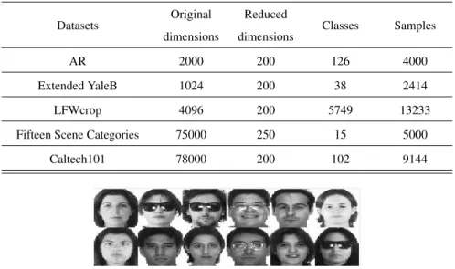
In this section, we evaluate our algorithm on several well-known databases (AR, Extended YaleB, LFWcrop, Fifteen Scene Categories and Caltech101) whose details 120
are presented in Table 1. We compare our method with PCA [28], LPP [11], NPE [14] and LRPP [21]. For LPP, NPE, LRPP and our method, we first use PCA to reduce dimensionality of all original datasets (except for Fifteen Scene Category database) to be 200, and then extract feature by these four methods, respectively. 1-nearest neighbor (1NN) is used for classification. We tune parameters for baseline methods by class-wise 125
cross-validation using the training data. In the following experiments, we perform ten rounds of random partitions for training and testing data and show the mean recognition rates and standard deviations. In addition, we also compare the recognition rate curves of different algorithms under different numbers of feature dimensions. All the above mentioned experiments were run on the windows-7 operating systems (Intel Core i7-130
4770 CPU M620 @ 3.40 GHz 8 GB RAM).
The AR database [29] contains over 4000 color face images of 126 people, in-cluding frontal views of faces with different facial expressions, lighting conditions and occlusions. The pictures of 120 individuals (65 men and 55 women) are taken in two sessions (separated by two weeks). Each session contains 13 color images, which in-135
Table 1: Descriptions of the benchmark datasets.
Datasets Original dimensions
Reduced
dimensions Classes Samples
AR 2000 200 126 4000
Extended YaleB 1024 200 38 2414
LFWcrop 4096 200 5749 13233
Fifteen Scene Categories 75000 250 15 5000 Caltech101 78000 200 102 9144
Figure 1: Some samples in the AR dataset.
Figure 2: Some samples in the Extended YaleB dataset.
Figure 3: Some samples in the LFWcrop dataset.
Figure 5: Some samples in the Caltech101 dataset.
and lighting conditions. In the experiments, we manually cropped the face portion of the image and then normalized it to 50×40. Figure 1 shows some images of the AR database. In this database, we randomly select 7 images per subject for training, and the remaining images for testing. Figure 10 shows the accuracy of our method vs 140
parameterαandβ. We can see that, whenα=0.7andβ=0.1, our method has good performance. Thus, in this dataset, we setα=0.7andβ=0.1and repeat the experiment 10 times.
The Extended YaleB database [30] consists of 2414 frontal-face images of 38 in-dividuals with the resolution and illumination changes. There are 64 images for each 145
object except 60 for 11th and 13th, 59 for 12th, 62 for 15th and 63 for 14th, 16th and 17th. In the experiments, we manually cropped the face portion of the image and then normalized it to 32×32. Figure 2 shows some images of this database. In this database, we randomly select 32 images per subject for training, and the remaining images for testing. In the experiments , we setα=5.3andβ=0.1. All of experiments are repeated 150
10 times.
The LFWcrop database [31] is a cropped version of the Labeled Faces in the Wild (LFW) [31] dataset, keeping only the center portion of each image (i.e. the face). In the vast majority of images, almost all of the backgrounds are omitted. The extracted area was then scaled to a size of 64x64 pixels. The selection of the bounding box 155
location was based on the positions of 40 randomly selected LFW faces [31]. As the location and size of faces in LFW were determined through the use of an automatic face locator (detector) [31], the cropped faces in LFWcrop exhibit real-life conditions, including misalignment, scale variations, in-plane as well as out-of-plane rotations. Some sample images are shown in Figure 3. In the experiment, we choose people who 160
57 classes and 1883 images. In the experiments, we setα=2.1andβ=0.1. For each person, we randomly choose ninety percent of images for training, and the remaining images for testing. We repeat this process 10 times.
The Fifteen Scene Categories database [32] includes 15 natural scene categories, 165
such as office, street, store and so on, as shown in Figure 4. Each category has 200 to 400 images, and the average image size is about250×300pixels. The major sources of the pictures in the database contain the COREL collection, personal photographs, and Google image search. It is one of the most complete scene category database used in the literature. We compute the spatial pyramid feature using a four-level spatial 170
pyramid and a SIFT-descriptor codebook with a size of 200. The final spatial pyramid features are reduced to 250 by PCA. We randomly select 20 images per category as training samples and use the rest as test samples. In the experiments, we setα=0.001 andβ=0.018. All of experiments are repeated 10 times.
The Caltech101 dataset [33] contains 9144 images from 102 classes (i.e., 101 object 175
classes and a background class) which include pizza, umbrella, watch, dolphin, and so on, as shown in Figure 5. The number of images of per class varies from 31 to 800. The vector quantization codes are pooled together to form a pooled feature in each spatial subregion of the spatial pyramid. We reduce the feature dimension to 200 by using PCA. Each class is randomly selected 20 images as training samples and the rest as test 180
samples. In the experiments , we setα=0.001andβ=0.019. All of experiments are repeated 10 times.
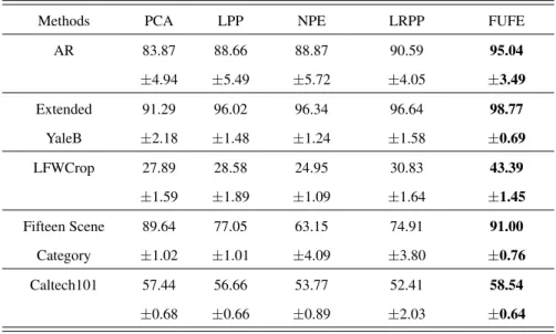
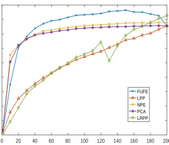
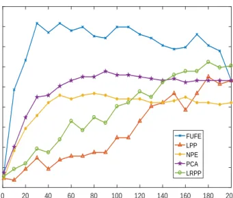
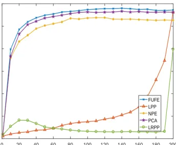
Figure 7 to Figure 11 show the average classification accuracy versus the number of feature dimension on the AR, Extended YaleB, LFWcrop, Fifteen Scene Categories and Caltech101 databases, respectively. Table 2 shows the average classification accuracy 185
and standard deviation on the five databases.
Comparing the aforementioned experiments, we have the several interesting obser-vations:
(1) Our method FUFE achieves the best average accuracy for all the cases. On the LFWcrop database, FUFE algorithm has obvious advantages compared with the other 190
methods. One possible reason may be that PCA, LPP and NPE assume that the projec-tion of data is exactly equal to the low-dimensional representaprojec-tion. This makes them
Table 2: The optimal average classification accuracy (%) and standard deviation on the AR, Extended Yale B, LFWcrop, Fifteen Scene Category and Caltech101 datasets.
Methods PCA LPP NPE LRPP FUFE
AR 83.87 88.66 88.87 90.59 95.04 ±4.94 ±5.49 ±5.72 ±4.05 ±3.49 Extended 91.29 96.02 96.34 96.64 98.77 YaleB ±2.18 ±1.48 ±1.24 ±1.58 ±0.69 LFWCrop 27.89 28.58 24.95 30.83 43.39 ±1.59 ±1.89 ±1.09 ±1.64 ±1.45 Fifteen Scene 89.64 77.05 63.15 74.91 91.00 Category ±1.02 ±1.01 ±4.09 ±3.80 ±0.76 Caltech101 57.44 56.66 53.77 52.41 58.54 ±0.68 ±0.66 ±0.89 ±2.03 ±0.64 β α 0 0.2 0.1 0.4 0.6 Accuracy 0.3 0.8 0.5 1 1.5 0.7 1.3 0.9 1.1 1.1 0.9 1.3 0.7 1.5 0.5 0.3 0.1
Figure 6: Accuracy of our method versus parametersαandβon the AR database.
fail to characterize the intrinsic geometric structure of data, which is important for data classification. Moreover, this strict constraint may result in over-fitting. Another
pos-0 20 40 60 80 100 120 140 160 180 200 Feature dimension 0 0.1 0.2 0.3 0.4 0.5 0.6 0.7 0.8 0.9
Recognition rate FUFE
LPP NPE PCA LRPP
Figure 7: Average recognition accuracyvs. number of projection vectors on the AR database.
0 20 40 60 80 100 120 140 160 180 200 Feature dimension 0 0.1 0.2 0.3 0.4 0.5 0.6 0.7 0.8 0.9 1 Recognition rate FUFE LPP NPE PCA LRPP
Figure 8: Average recognition accuracyvs. number of projection vectors on the Extended YaleB database.
sible reason is that we add a regression residual termXTW−F2
F in our objective
195
0 20 40 60 80 100 120 140 160 180 200 Feature dimension 0 0.05 0.1 0.15 0.2 0.25 0.3 0.35 0.4 0.45 Recognition rate FUFE LPP NPE PCA LRPP
Figure 9: Average recognition accuracyvs. number of projection vectors on the LFWcrop database.
0 50 100 150 200 250 Feature dimension 0 0.1 0.2 0.3 0.4 0.5 0.6 0.7 0.8 0.9 Recognition rate FUFE LPP NPE PCA LRPP
Figure 10: Average recognition accuracyvs. number of projection vectors on the Fifteen Scene Category database.
0 20 40 60 80 100 120 140 160 180 200 Feature dimension 0 0.1 0.2 0.3 0.4 0.5 0.6 Recognition rate FUFE LPP NPE PCA LRPP
Figure 11: Average recognition accuracyvs. number of projection vectors on the Caltech101 database.
that our method is generally suitable to cope with a certain type of nonlinear manifold that is somewhat close to a linear subspace.
(2) PCA performs better than LPP and NPE in the Fifteen Scene Category database and Caltech101 database. This is probably due to the fact that the graph, which is 200
artificially constructed in LPP and NPE in these two datasets, does not well characterize the intrinsic geometric structure of data [27]. Our method is superior to PCA, LPP, NPE and LRPP, the reason may be that FUFE well preserves both local and global geometric structures of data.
(3) In the face datasets (AR, Extended YaleB and LFWcrop), LRPP is superior to 205
PCA, LPP and NPE. This is attributed to the fact that LRPP adaptively learns similar-ity matrix which determines the construction of graph. In the fifteen scene category database and Caltech101 database, LRPP is inferior to the other methods. The reason may be that LRPP does not reveal global geometric structure of data. According to Figure 10 and Figure 11, it is easy to see that the recognition accuracy has a sharp in-210
crease when the dimension is close to the peak. Different from face images, the feature on the fifteen scene category database or Caltech101 database may not be suited for
low rank representation so that LRPP cannot learn a well low-rank weight matrix es-pecially when the dimension of features is low. In the future, we will study the change of recognition rate of LRPP in higher dimensions.
215
(4) As can be seen in Figure 10, Figure 11 and Table 2, all methods (PCA, LP-P, NPE, LRPP and FUFE) do not achieve a good recognition rate on the LFWcrop and Caltech101 databases. This is probably because that LFWcrop and Caltech101 databases consist of natural portrait without setting conditions. It is very challenging for subspace learning methods.
220
5. Conclusions
In this paper, we propose a flexible unsupervised dimensionality method for fea-ture extraction. Different from most existing dimensionality reduction methods, our method uses an elastic constraint on the projection such that it can well reveal geo-metric structure of data. Thus, our method is not only suitable for dealing with certain 225
types of nonlinear manifolds, but also can effectively characterize both local and glob-al geometric structures. Moreover, theoreticglob-al anglob-alysis proves that PCA and LPP are special cases of the proposed model. Finally, a non-iterative algorithm is proposed to solve our model. Experiments on several well-known databases (AR, Extended Yale-B, LFWcrop, Fifteen Scene Categories and Caltech101) illustrate the efficiency of our 230
proposed approach. In the future, our main work is to combine proposed model with convolutional neural networks for handling gesture recognition, behavior recognition and other applications.
Acknowledgment
The authors would like to thank the anonymous reviewers and AE for their con-235
structive comments and suggestions, which improved the paper substantially. This work is supported by National Natural Science Foundation of China under Grant 61773302 and the 111 Project of China (B08038).
References
[1] Z. Li, J. Liu, J. Tang, H. Lu, Robust structured subspace learning for data rep-240
resentation, IEEE Transactions on Pattern Analysis and Machine Intelligence 37 (10) (2015) 2085–2098.
[2] Y. Liu, Q. Gao, S. Miao, X. Gao, F. Nie, Y. Li, A non-greedy algorithm for l1-norm lda, IEEE Transactions on Image Processing 26 (2) (2016) 684–695. [3] M. Jiang, W. Huang, Z. Huang, G. G. Yen, Integration of global and local metrics 245
for domain adaptation learning via dimensionality reduction, IEEE transactions on cybernetics 47 (1) (2017) 38–51.
[4] X. Lan, A. J. Ma, P. C. Yuen, R. Chellappa, Joint sparse representation and robust feature-level fusion for multi-cue visual tracking, IEEE Transactions on Image Processing 24 (12) (2015) 5826–5841.
250
[5] T. Zhou, H. Bhaskar, F. Liu, J. Yang, Graph regularized and locality-constrained coding for robust visual tracking, IEEE Transactions on Circuits and Systems for Video Technology 27 (10) (2017) 2153–2164.
[6] J. Zheng, Z. Jiang, R. Chellappa, Cross-view action recognition via transferable dictionary learning, IEEE Transactions on Image Processing 25 (6) (2016) 2542– 255
2556.
[7] B. Fernando, E. Gavves, J. Oramas, A. Ghodrati, T. Tuytelaars, Rank pooling for action recognition, IEEE transactions on pattern analysis and machine intelli-gence 39 (4) (2017) 773–787.
[8] M. Turk, A. Pentland, Eigenfaces for recognition, Journal of cognitive neuro-260
science 3 (1) (1991) 71–86.
[9] P. N. Belhumeur, J. P. Hespanha, D. J. Kriegman, Eigenfaces vs. fisherfaces: recognition using class specific linear projection, IEEE Transactions on Pattern Analysis and Machine Intelligence 19 (7) (2002) 711–720.
[10] M. Belkin, P. Niyogi, Laplacian eigenmaps for dimensionality reduction and data 265
representation, Neural computation 15 (6) (2003) 1373–1396.
[11] X. Niyogi, Locality preserving projections, in: Neural information processing systems, Vol. 16, Vancouver, Canada, 2004, pp. 153–159.
[12] Y. Liu, S. Zhao, Q. Wang, Q. Gao, Learning more distinctive representation by enhanced pca network, Neurocomputing 275 (2018) 924–931.
270
[13] Y. Liu, Q. Gao, X. Gao, L. Shao, L21-norm discriminant manifold learning, IEEE Access 6 (2018) 40723–40734.
[14] X. He, D. Cai, S. Yan, H.-J. Zhang, Neighborhood preserving embedding, in: IEEE International Conference on Computer Vision, Vol. 2, IEEE, Beijing, China, 2005, pp. 1208–1213.
275
[15] S. T. Roweis, L. K. Saul, Nonlinear dimensionality reduction by locally linear embedding, Science 290 (5500) (2000) 2323–2326.
[16] N. Shahid, V. Kalofolias, X. Bresson, M. Bronstein, Robust principal component analysis on graphs, in: IEEE International Conference on Computer Vision, 2015, pp. 2812–2820.
280
[17] S. Liao, J. Li, Y. Liu, Q. Gao, X. Gao, Robust formulation for pca: Avoiding mean calculation with l2, p-norm maximization., in: AAAI, 2018.
[18] H. Luo, Y. Y. Tang, C. Li, L. Yang, Local and global geometric structure preserv-ing and application to hyperspectral image classification, Mathematical Problems in Engineering 2015.
285
[19] D. Cai, X. He, K. Zhou, J. Han, H. Bao, Locality sensitive discriminant analysis., in: IJCAI, 2007, pp. 708–713.
[20] Y. Xu, X. Fang, J. Wu, X. Li, D. Zhang, Discriminative transfer subspace learning via low-rank and sparse representation, IEEE Transactions on Image Processing 25 (2) (2016) 850–863.
[21] Y. Lu, Z. Lai, Y. Xu, X. Li, D. Zhang, C. Yuan, Low-rank preserving projections, IEEE Trans. Cybernetics 46 (8) (2016) 1900–1913.
[22] S. Yan, D. Xu, B. Zhang, H.-J. Zhang, Q. Yang, S. Lin, Graph embedding and extensions: a general framework for dimensionality reduction, IEEE Transactions on Pattern Analysis and Machine Intelligence 29 (1) (2007) 40–51.
295
[23] Y. Huang, D. Xu, F. Nie, Semi-supervised dimension reduction using trace ratio criterion, IEEE Transactions on Neural Networks and Learning Systems 23 (3) (2012) 519–526.
[24] Y. Liu, Y. Guo, H. Wang, F. Nie, H. Huang, Semi-supervised classifications via elastic and robust embedding., in: Proceedings of the Thirty-First AAAI Confer-300
ence on Artificial Intelligence, 2017, pp. 2294–2330.
[25] J. Chen, J. Ye, Q. Li, Integrating global and local structures: A least squares framework for dimensionality reduction, in: IEEE Conference on Computer Vi-sion and Pattern Recognition, 2007, pp. 1–8.
[26] D. Cai, X. He, J. Han, Semi-supervised discriminant analysis, in: IEEE Interna-305
tional Conference on Computer Vision, 2007, pp. 1–7.
[27] Q. Gao, J. Ma, H. Zhang, X. Gao, Y. Liu, Stable orthogonal local discriminant embedding for linear dimensionality reduction, IEEE Transactions on Image Pro-cessing 22 (7) (2013) 2521–2531.
[28] M. Turk, A. Pentland, Eigenfaces for recognition, Journal of cognitive neuro-310
science 3 (1) (1991) 71–86.
[29] A. M. Martinez, The ar face database, CVC Technical Report 24.
[30] A. S. Georghiades, P. N. Belhumeur, D. J. Kriegman, From few to many: Illumi-nation cone models for face recognition under variable lighting and pose, IEEE Transactions on Pattern Analysis and Machine Intelligence 23 (6) (2001) 643– 315
[31] C. Sanderson, B. C. Lovell, Multi-region probabilistic histograms for robust and scalable identity inference, in: International Conference on Biometrics, Springer, 2009, pp. 199–208.
[32] S. Lazebnik, C. Schmid, J. Ponce, Beyond bags of features: Spatial pyramid 320
matching for recognizing natural scene categories, in: IEEE Conference on Com-puter Vision and Pattern Recognition, 2006, pp. 2169–2178.
[33] L. Fei-Fei, R. Fergus, P. Perona, Learning generative visual models from few training examples: An incremental bayesian approach tested on 101 object cate-gories, Computer Vision and Image Understanding 106 (1) (2007) 59–70. 325