Hedging for the Long Run

(1)

QUANTITATIVE FINANCE

RESEARCH CENTRE

��

QUANTITATIVE FINANCE RESEARCH CENTRE

Research Paper 214 February 2008

Hedging for the Long Run

Hardy Hulley and Eckhard Platen

(2)

HEDGING FOR THE LONG RUN

ECKHARD PLATEN AND HARDY HULLEY

Abstract. In the years following the publication of Black and Sc-holes [7], numerous alternative models have been proposed for pricing and hedging equity derivatives. Prominent examples include stochas-tic volatility models, jump diffusion models, and models based on L´evy processes. These all have their own shortcomings, and evidence sug-gests that none is up to the task of satisfactorily pricing and hedging extremely long-dated claims. Since they all fall within the ambit of risk-neutral pricing, it is thus natural to speculate that their deficiencies are (at least in part) attributable to the modelling constraints imposed by the risk-neutral approach itself. To investigate this idea, we present a simple two-parameter model for a diversified equity accumulation index. Although our model does not admit an equivalent risk-neutral probabil-ity measure, it nevertheless fulfils a minimal no-arbitrage condition for an economically viable financial market. Furthermore, we demonstrate that contingent claims can be priced and hedged, without the need for an equivalent change of probability measure. Convenient formulae for the prices and hedge ratios of a number of standard European claims are derived, and a series of hedge experiments for extremely long-dated claims on the S&P 500 total return index are conducted. Our model serves also as a convenient medium for illustrating and clarifying several points on asset price bubbles and the economics of arbitrage.

JEL Classification: G10, G12, G13.

Keywords: Long-dated claims; risk-neutral pricing; real-world pricing;

arbitrage; minimal market model; squared Bessel processes; hedge sim-ulations; asset price bubbles.

Date: February 12, 2008.

(3)

1. Introduction

It is widely acknowledged that the current generation of equity deriva-tive pricing models display several shortcomings, the consequences of which become progressively more severe as one attempts to price and hedge con-tracts with longer maturities. This scaling of model risk with maturity has contributed to a number of high-profile losses in the equity options mar-kets. For example, in 1997 Union Bank of Switzerland (UBS) is said to have suffered a loss of at least 100 million Swiss francs due to the impact of a model error on written long-dated equity options [see 38]. The spectacular losses by Long-Term Capital Management (LTCM) in 1998 were also largely attributable to short positions in long-dated S&P 500 equity index options, which accounted for losses of some 1.3 billion US dollars [see 29].

To exemplify some of the above-mentioned shortcomings, we start with the prototype of all stochastic asset pricing models, namely the Black and Scholes [7] (BS) model. Its inadequacies were quickly apparent, when it was observed that the volatilities implied by traded options with different strikes and maturities form a curved surface, which is inconsistent with the constant volatility assumption of the model itself. In an effort to redress this anomaly, substantial research has been devoted to stochastic volatility models [see e.g. 19, 21, 42]. The basic idea is to keep the dynamics of the underlying stock price or index substantially the same as the BS model, but to allow the volatility to follow a separate (possibly correlated) diffusion process. An adequately parameterized stochastic volatility model can then be calibrated to the observed implied volatility surface.

Another unrealistic feature of the BS model is the implicit assumption of normally distributed log-returns, which is at odds with the asymmetric leptokurtic features of observed equity returns. A possible remedy for these distributional problems is to augment the underlying diffusion model with finite intensity jumps, resulting in the family of jump-diffusion models [see e.g. 24, 31]. Hybrid models, incorporating stochastic volatility in a jump-diffusion framework, have also been considered [see e.g. 5, 14].

A more recent idea has been to abandon the diffusion component of eq-uity models completely. The realization that diffusive behaviour may be captured adequately by jump processes with infinite arrival rates has stim-ulated the development of asset pricing models based on infinite activity pure jump L´evy processes [see e.g. 4, 9, 17, 30]. The common drawback of these models is an inability to capture the observed variation of option prices across maturity. To remedy this, Carr et al. [10] recently extended a number of them, by incorporating a mean-reverting stochastic volatility.

Although each of the models surveyed above attempts to redress the de-ficiencies of the BS model in a different way, they all have at least one thing in common—they fit into the prevailing risk-neutral valuation paradigm. This paper, by contrast, explores the notion that perhaps the risk-neutral approach itself is (at least part of) the problem. In particular, we ask the reader to consider the possibility that the required existence of an equiv-alent risk-neutral probability measure imposes an unrealistic constraint on modelling freedom that is significant enough to affect long-term pricing and

(4)

hedging performance adversely. We anticipate two immediate objections to our proposal, which we briefly address.

Firstly, it is well-known that the existence of an equivalent risk-neutral probability measure is necessary and sufficient to preclude arbitrage oppor-tunities of a certain type [see e.g. 13]. Therefore, by considering models that do not fit into the risk-neutral framework, we are implicitly exposing our-selves to some sort of arbitrage. In response to this, we note that recent work has systematically played down the importance of arbitrage in asset pricing. For example, Shleifer and Vishny [39] showed that when arbitrage oppor-tunities require capital, they may be ineffective in bringing security prices back to fundamental values—especially under conditions of extreme mis-pricing. Furthermore, professional arbitrageurs may in fact avoid volatile arbitrage strategies altogether—even when the expected returns are very tempting—for fear of being forced by their investors to liquidate under ad-verse conditions. More recently, Liu and Longstaff [27] have demonstrated that risk-averse investors will under-invest in arbitrage opportunities with the potential of yielding negative interim returns, if liabilities must be se-cured by collateral (as is the case in reality). We also draw attention to Loewenstein and Willard [28], where it was argued that for a financial mar-ket to admit competitive equilibrium prices, only a minimal no-arbitrage condition (see Definition 1) is required. In general, this condition is in-sufficient to ensure the existence of an equivalent risk-neutral probability measure.

The second objection is practical by nature. If a model does not conform to the risk-neutral approach, how can it be used to price and hedge contin-gent claims? To address this question, we present a simple two-parameter model for a market comprising a diversified equity accumulation index1_{and a}

deterministic savings account. Although our model does not admit an equiv-alent risk-neutral probability measure, claims on the index can be priced by computing expectations under the real-world probability measure, when the index itself is chosen as num´eraire [see 18]. The prices obtained in this way are minimal, in the sense of being the smallest possible initial endowments for successful hedge portfolios.

Having examined some of the arguments against our proposed relaxation of the risk-neutral constraint, we briefly present some evidence in its favour. Figure 1 plots the ratio of a US dollar savings account to the S&P 500 total return index, over the 86-year period from January 1920 until Decem-ber 2006. The index was constructed from monthly data supplied by Global Financial Data and Thomson Datastream, while the savings account was obtained by rolling over an initial investment in 30-day US treasury bills, chosen to make the ratio start at one. The feature of this graph we wish to highlight is its systematic long-term decline2_{. If an equivalent risk-neutral}

probability measure for the index exists, then the curve in Figure 1 is a nat-ural proxy for its density process [see 34, Sec 9.4 and Sec. 10.6], and should therefore be a sample path of a martingale. Although we only have access

1_{We specify an accumulation index to avoid having to model dividends explicitly.} 2_{Of course, this is unsurprising, since conventional wisdom holds that equities outperform}

debt in the long run.

(5)

to one history, it seems implausible that this is the case. It is rather more likely that the process is in fact a strict supermartingale, and is thus not the density for any equivalent change of probability measure3_.

0 10 20 30 40 50 60 70 80 90 0 0.2 0.4 0.6 0.8 1 1.2 1.4 1.6 1.8

Putative Risk−Neutral Density Process

Time

Density

Figure 1. The path of the putative risk-neutral density pro-cess over the period January 1920–December 2006.

A final observation concerning Figure 1 is that the steady downward trend is readily apparent only over long time-frames. Over relatively short periods—less than three years, say—it is not generally noticeable. In other words, the putative density process may indeed approximate the behaviour of a martingale for a limited time. In this case, the impact of its hypoth-esized strict supermartingale character on pricing and hedging should be most significant for very long-dated claims. The obvious corollary is that models falling within the risk-neutral framework may be adequate for pric-ing and hedgpric-ing derivatives with short maturities, even if there is in fact no equivalent risk-neutral probability measure. It is natural to wonder whether some of the well-publicized trading losses associated with short positions in long-dated equity volatility may in part be attributable to a failure of the risk-neutral approach over long time-spans.

We end this introduction with a synopsis of the remainder of the paper. Section 2 presents our model for a large diversified equity accumulation in-dex, and discusses its arbitrage implications. In Section 3 we show how to price claims written on the index, even though the model does not admit an equivalent risk-neutral probability measure. We also demonstrate that dynamic hedging is possible, and present formulae for the prices and hedge ratios of a number of standard European claims. Section 4 considers the

3_{If the ratio plotted in Figure 1 is a sample path of a strict supermartingale, then the}

corresponding process is what Kramkov and Schachermayer [25], Sec. 2 refer to as a strict supermartingale density. In other words, it is the density process for an equivalent change of measure, but the resulting measure is deficient.

(6)

problem of parameter estimation, and outlines a simple technique for ob-taining parameter values. We then use 30-day US treasury bill rates and the S&P 500 total return index, over the period January 1920–December 2006, to obtain parameter estimates for our model. Using these estimates, to-gether with the above-mentioned interest rate and index data, Section 5 conducts a series of hedge simulations for claims written on the index. The salient feature of these simulations is the extreme initial maturities of the claims—equal to the full 86-year span of the data. As intimated earlier, we are interested in hedging performance over the extreme long-term, since it is over the long run that the hypothesized strict supermartingale property of Figure 1 should have the most dramatic effect. Finally, Section 6 draws some conclusions, while three technical appendices are included to keep the presentation self-contained. These present an overview of squared Bessel processes, prove a proposition stated in Section 3, and derive the pricing formulae in Section 3, respectively.

2. The Model

We specify a market comprising a savings account B = (Bt)t≥0 and a

diversified equity accumulation index S = (St)t≥0. The savings account is

given by Bt:= exp µZ _t 0 r(s)ds ¶ ,

where r(·) is a deterministic instantaneous short rate. We model the index under the real-world probability measure P, as a solution to the stochastic differential equation (SDE)

dSt=

¡

r(t) +θ2(t, St)

¢

Stdt+θ(t, St)StdWt, (1)

where W = (Wt)t≥0 is a standard Brownian motion underP, θ(t, St) :=

s

αexp(ηt)Bt

St (2)

is a local volatility function, and α, η > 0 are fixed parameters. Equa-tions (1)–(2) are referred to as the minimal market model (MMM), first introduced in Platen [32]. Note that in this model the risk premium for the index is the square of its volatility, and its Sharpe ratio is its volatility.

The parameters α and η in (2) may be interpreted as a scaling factor and the growth rate of the index in excess of the risk-free rate, respectively. The local volatility function (2) is similar to that of the constant elasticity of variance (CEV) model considered in Cox and Ross [12], Eq. (7). In particular, the MMM exhibits some form of the leverage effect described by Black [6]. Notice, however, that in the MMM volatility is replenished at a rate of pexp(ηt)Bt. This remedies one of the structural defects of

the CEV model, where volatility systematically vanishes along increasing sample paths, until they are essentially deterministic.

Let ¯St:=St/Bt denote the discounted index. An application of Itˆo’s

for-mula reveals that ¯S = ( ¯St)t≥0 is a time-transformed squared Bessel process

of dimension four:

¯

St(d)= Xϕ(t), (3)

(7)

where

ϕ(t) := α

4η[exp(ηt)−1] (4)

is a deterministic time transformation, andX= (Xt)t≥0 is a squared Bessel

process of dimension four (see Appendix A). This representation is impor-tant for obtaining convenient formulas for option prices and hedge ratios, since the transition densities of squared Bessel processes are known.

An important feature of the MMM we wish to highlight is that it does not accommodate an equivalent risk-neutral probability measure. The following intuitive argument makes this clear: Even though the volatility (2) of the index grows without bound as it approaches zero, it follows from (1) that its drift grows even faster, exerting a repulsive force away from the origin. However, the index drift would be linear under any hypothetical risk-neutral probability measure, and so exploding volatility close to the origin would cause some sample paths to hit zero. Thus the index would have a non-zero risk-neutral probability of hitting zero, while the real-world probability of this event is zero.

There is, of course, a well-established correspondence between the absence of arbitrage, in the guise of the no free lunch with vanishing risk (NFLVR) condition, and the existence of an equivalent risk-neutral probability mea-sure [see 13]. In the light of the previous paragraph, it is thus natural to enquire about the arbitrage implications of (1)–(2). To address this ques-tion, let π = (πt)t≥0 denote the fraction of wealth held in the index by a

self-financing portfolio comprising the index and the savings account. Its value Sπ _{= (}_Sπ

t)t≥0 satisfies the following SDE: dS_tπ =¡r(t) +πtθ2(t, St)

¢

S_tπdt+πtθ(t, St)StπdWt. (5)

It then follows that the benchmarked portfolio value ˆSπ ₌¡_Sˆπ t

¢

t≥0, defined

by ˆS_tπ :=S_tπ/St, is a local martingale, since Itˆo’s formula gives

dSˆ_tπ =−(1−πt)θtSˆtπdWt. (6)

If we stipulate further thatSπ

t ≥0, then ˆSπ is a non-negative

supermartin-gale, by Fatou’s lemma [see e.g. 36, Lem. 14.3, p. 22]. Consequently, if ˆSπ

ever vanishes, it must remain zero [see e.g. 26, Note 2 to Th. 3.5, p. 62]. We have thus established that the MMM excludes arbitrage opportunities of the following type [see 28, 33]:

Definition 1. An arbitrage is a non-negative self-financing portfolio Sπ

satisfying

P¡S_uπ = 0¢= 1 and P¡S_tπ >0¢>0,

for some 0≤u < t.

One may argue that excluding this strong form of arbitrage is the mini-mal condition for sustaining a realistic financial market in which investors can make well-defined optimal decisions, even though it does not guarantee the existence of an equivalent risk-neutral probability measure. For exam-ple, Loewenstein and Willard [28] demonstrate that under this no-arbitrage condition financial markets admit competitive equilibria. Also, Platen and Heath [34] argue that its enforcement at an institutional level is precisely

(8)

the role of financial regulators, who must ensure that market participants remain going concerns.

3. Pricing and Hedging

Fix a finite maturity T > 0, and let h(·) be a non-negative payoff func-tion which is not identically zero and satisfiesE[h(ST)/ST]<∞, whereE[·]

denotes expectation under P. Our objective in this section is to price and hedge a European contingent claim paying h(ST) at maturity. Although

risk-neutral pricing is unavailable to us, (6) indicates that the index is a num´eraire for the real-world probability measure. Following Geman et al. [18], we thus propose that the value of the claim Vh_{= (}_Vh

t )0≤t≤T be

deter-mined by the following real-world pricing formula:

V_th=Vh(t, St) :=StE · h(ST) ST ¯ ¯ ¯ ¯St ¸ . (7)

Of course, Geman et al. [18] work in the context of a market that supports an equivalent risk-neutral probability measure. One of their main results justifies pricing with respect to a general num´eraire, by demonstrating its consistency with risk-neutral pricing. Our justification for (7) cannot depend on risk-neutral pricing. Instead, we start by observing that the price process

Vh _{can be replicated by a self-financing strategy (see Appendix B for a}

proof).

Definition 2. Letπ = (πt)0≤t≤T be a self-financing strategy. We shall say

that Sπ _{hedges the claim if} _Sπ

T =h(ST), and that it replicates the value of

the claim if Sπ

t =Vth, at all timest∈[0, T].

Proposition 3. Define the self-financing strategy πh _{= (}_πh

t)0≤t≤T, by set-ting πh_t =πh(t, St) := _V_h₍S_{t, S}t t) ∂Vh ∂S (t, St). (8)

The associated self-financing portfolio Sπh = ¡S_tπh¢₀_≤_t_≤_T, with initial en-dowment Sπh

0 :=S0E £

h(ST)/ST

¤

, then replicates the value of the claim.

An immediate consequence of the above result is thatSπhhedges the claim as well, since Sπ_Th = V_Th = h(ST). Now consider any other self-financing

strategyπ, such thatSπ _{hedges the claim. It follows from Proposition 3 and}

(7) that ˆSπh

t :=Sπ

h

t /St=Vth/Stdefines a (uniformly integrable) martingale

ˆ Sπh =¡Sˆπh t ¢ 0≤t≤T. Hence S_tπh=StSˆπ h t =StE h ˆ S_Tπh ¯ ¯ ¯St i =StE · h(S_T) ST ¯ ¯ ¯ ¯St ¸ =StE h ˆ S_Tπ ¯ ¯ ¯St i ≤StSˆtπ =Stπ, (9)

as a consequence of the supermartingale property of ˆSπ. So not only is (7) the value of a portfolio that hedges the claim, it is the value of the cheapest hedge portfolio. This is our justification of real-world pricing.

(9)

Contingent Claim Payoff Pricing Function Zero coupon bond 1 Z(t, S)

European call (ST −K)+ C(t, S)

European put (K−ST)+ P(t, S)

Binary European call I_{_S_T_≥_K_} BC(t, S) Binary European put I_{_K_≥_S_T_} BP(t, S)

Table 1. The instruments under consideration.

Table 1 lists the payoffs of a few common European claims, as well as their associated pricing functions. The expressions for these functions, presented below, are obtained by evaluating (34) in Appendix C, in each case:

Z(t, S) = Bt B_T · 1−exp ³ −1 2λ(t, S) ´¸ ; (10) C(t, S) =S h 1−Ψ¡x(t); 4, λ(t, S)¢i −KBt B_T h 1−Ψ¡x(t); 0, λ(t, S)¢i; (11) P(t, S) =KBt BT · Ψ¡x(t); 0, λ(t, S)¢−exp ³ −1 2λ(t, S) ´¸ −SΨ¡x(t); 4, λ(t, S)¢; (12) BC(t, S) = Bt BT h 1−Ψ¡x(t); 0, λ(t, S)¢i; (13) and BP(t, S) = Bt B_T · Ψ¡x(t); 0, λ(t, S)¢−exp ³ −1 2λ(t, S) ´¸ . (14)

In the expressions above

Ψ(x;ν, λ) :=P£χ2_ν(λ)≤x¤,

where χ2

ν(λ) is a non-central chi-square random variable with ν degrees of

freedom and non-centrality λ, while

λ(t, S) := S/Bt ∆ϕ(t) and x(t) := K/B_T ∆ϕ(t), (15) with ∆ϕ(t) :=ϕ(T)−ϕ(t). (16) Detailed derivations of (10)–(14) are provided in Appendix C.

It is interesting to note that even though the MMM does not admit an equivalent risk-neutral probability measure, the basic put-call parity rela-tions still hold:

C(t, S) +KZ(t, S) =P(t, S) +S and BC(t, S) +BP(t, S) =Z(t, S).

The crucial—though perhaps counter-intuitive—observation is that a zero-coupon bond is now an equity index derivative. Its value is obtained from the real-world pricing formula, and not by discounting at the risk-free rate.

(10)

As Proposition 3 demonstrates, in order to hedge the claim, we must calculate its delta

∆h(t, S) := ∂Vh

∂S (t, S).

To do this for the pricing functions (11)–(14), we make use of the following identity [see 23, Eq. (29.23d), p. 442]:

∂Ψ ∂λ(x;ν, λ) = 1 2 £ Ψ(x;ν+ 2, λ)−Ψ(x;ν, λ)¤. (17) The following deltas are obtained for the claims listed in Table 1:

∆Z(t, S) = 1₂_BBt T ∂λ ∂S(t, S) exp ³ −1 2λ(t, S) ´ ; (18) ∆_C(t, S) = 1− 1 2S ∂λ ∂S(t, S)Ψ ¡ x(t); 6, λ(t, S)¢ + µ 1 2S ∂λ ∂S(t, S)−1 ¶ Ψ¡x(t); 4, λ(t, S)¢ +1 2K Bt B_T ∂λ ∂S(t, S) h Ψ¡x(t); 2, λ(t, S)¢ −Ψ¡x(t); 0, λ(t, S)¢i; (19) ∆_P(t, S) =−1 2S ∂λ ∂S(t, S)Ψ ¡ x(t); 6, λ(t, S)¢ + µ 1 2S ∂λ ∂S(t, S)−1 ¶ Ψ¡x(t); 4, λ(t, S)¢ +1 2K Bt BT ∂λ ∂S(t, S) · Ψ¡x(t); 2, λ(t, S)¢ −Ψ¡x(t); 0, λ(t, S)¢−exp ³ −1 2λ(t, S) ´¸ ; (20) ∆_BC(t, S) = 1 2 Bt B_T ∂λ ∂S(t, S) h Ψ¡x(t); 0, λ(t, S)¢ −Ψ¡x(t); 2, λ(t, S)¢i; (21) and ∆BP(t, S) = 1 2 B_t BT ∂λ ∂S(t, S) · Ψ¡x(t); 2, λ(t, S)¢ −Ψ¡x(t); 0, λ(t, S)¢+ exp ³ −1 2λ(t, S) ´¸ . (22)

Fortunately, efficient algorithms exist for computing the non-central chi-square distribution function [see e.g. 23, Chap. 29, and the references therein], making the pricing and hedging formulas (10)–(14) and (18)–(22) compu-tationally feasible. For the empirical results in this paper, we implemented a slightly modified version of the algorithm presented in Schroder [37]. Its outputs are generally accurate to six decimal places, and the execution time is negligible. We also mention that with the aid of (17) and similar recur-sions presented in [23], all the familiar price sensitivities can be expressed in terms of non-central chi-square distributions.

(11)

It is interesting to note that the MMM is a natural vehicle for illustrating and clarifying several points in the contemporary literature concerning the economics of arbitrage and bubbles in financial markets. For example, Liu and Longstaff [27] recently considered a market comprising a risky portfolio

A= (At)0≤t≤T and a risk-free savings account, with the former modelled as

a Brownian bridge-type process satisfying AT = 0. Although their market

offers an arbitrage opportunity, in the classical sense4 _{of Dybvig and Huang}

[16], their main result nevertheless demonstrates that an investor with loga-rithmic5 preferences will tend to under-invest in it, when collateral must be posted against interim losses. The MMM provides a concrete example of the situation investigated by Liu and Longstaff [27]: By simultaneously invest-ing in the replicatinvest-ing portfolio for the zero-coupon bond and short-sellinvest-ing 1/B_T units of the savings account, we obtain a portfolio A = (At)0≤t≤T,

whose value at time t∈[0, T) is A_t= exp¡−1

2λ(t, St) ¢

>0, and which sat-isfies AT = 0. We conjecture that their characterization of optimal investor

behaviour in the face of collateralized borrowing will continue to hold. Another issue of contemporary importance, to which the MMM con-tributes some insight, concerns the unanticipated prevalence of strict local martingales in financial market models [see e.g. 3, 11, 41]. A systematic study of this phenomenon—in which strict local martingale behaviour is as-sociated with asset price bubbles—has recently been conducted by Heston et al. [20]. Using their terminology, the MMM exhibits a money market bubble6_{. We hesitate to subscribe to this terminology, however, since}

bub-bles are generally perceived as irrational, short-lived and anomalous. In our view, the idea that the payoff of a long-dated zero-coupon bond may be replicated for less than its discounted value, by trading in a diversified equity portfolio, is not strange. Rather, we see it as a manifestation of the commonplace observation that equities systematically outperform debt, in the long run. Far from being a bubble, this phenomenon is a stable, per-sistent feature of equity markets, with (we believe) a sound economic basis. We hope the hedge simulation results in Section 5 lend some weight to this opinion.

4. Parameter Estimation

There is an extensive literature on estimation for diffusions [see e.g. 2, 15]. However, instead of an established estimation procedure, we shall exploit a structural feature of the MMM to estimateα and η. The feature alluded to is the following representation of the time transform (4), obtained by using

4_{This is a portfolio with initial value zero, which is uniformly bounded below, and whose}

terminal value is non-negative with a positive probability of being strictly positive. Of course, this perforce means that the Liu and Longstaff model cannot accommodate an equivalent risk-neutral probability measure.

5_{In fact, the authors conjecture that the same result should apply for virtually all investors}

with risk-averse preferences.

6_{If rolling over an initial investment in the savings account is not the cheapest way of}

replicating the payoff of a zero-coupon bond, then Heston et al. [20] say there exists a money market bubble. This is clearly the case with the MMM, since Z(t, St)< Bt/BT,

(12)

Itˆo’s formula to derive the SDE for pS¯t from (1):

ϕ(t) =DpS¯ E

t. (23)

Given observation times 0 =t0 < t1 < . . . < tN, we now set

QVar_n:= n X i=1 µq ¯ S_t_i− q ¯ S_t_i₋₁ ¶₂ , (24)

for n≤N. Since QVarn converges in probability to the quadratic variation

√

¯

S®_t

n, as the maximum distance between the observation times decreases

to zero, (23) forms the basis for the following least-squares estimate of α

and η: (ˆα,ηˆ) = arg min (α,η) N X n=1 ³ QVar_n−ϕ(t_n) ´₂ . (25)

To demonstrate that this produces reasonable results, we chose the realistic parameter values S0 = 1, α = 0.01 and η = 0.05 to simulate 10,000 sample

paths of the discounted index. This was done using (3) and the fact that a squared Bessel process of dimension four can be simulated exactly by generating four independent Brownian motions, as discussed in Appendix A. Equation (25) was then used to estimate αandη along each path. To make the simulations compatible with our empirical data (described in the next paragraph), the paths contained only monthly samples over 86 years. The histograms in Figure 2 display the distributions of the parameter estimates. Without entering into a detailed statistical analysis, we report that the mean parameter estimates wereµαˆ = 0.010092 andµηˆ= 0.050002, with respective

variances σ2 ˆ

α= 2.2466×10−6 andση2ˆ= 7.2716×10−6. These results appear

to support our simple estimation procedure.

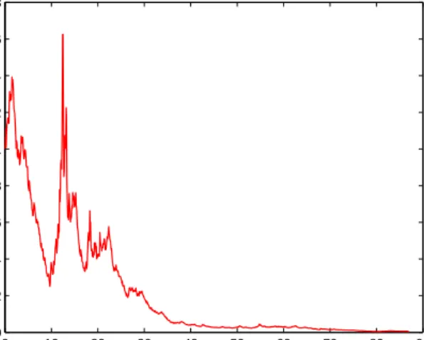
Finally, we applied the technique outlined above to the problem of es-timating the MMM for some empirical data. This consisted of a savings account generated from 90-day US T-Bill rates, as well as the S&P 500 total return index, sampled monthly over the period from January 1920 to De-cember 2006. The initial value of the index was 0.3865, and it finished at 2149.8, while the savings account, which was normalized to start with value one, finished at 27.982. The estimated parameter values were ˆα= 0.0035674 and ˆη = 0.055325. Figure 3 shows how well the fitted time transformation

ϕ(t) matches the approximate observed quadratic variation√S¯®_t, obtained from (24).

5. Hedge Simulations

This section presents the results of a hedge simulation experiment, which tested the pricing and hedging performance of the MMM for extreme ma-turity options on the S&P 500 total return index. We considered all the instruments listed in Table 1, with a common maturity of 86 years, which was the extent of our empirical data. The model was first fitted using the parameter values estimated in Section 4, after which the initial values of

(13)

0.0040 0.006 0.008 0.01 0.012 0.014 0.016 0.018 0.02 100 200 300 400 500 600

Estimated values for α

0.040 0.045 0.05 0.055 0.06 0.065 100 200 300 400 500 600 700

Estimated values for η

Figure 2. Parameter estimates for simulated paths of ¯St.

0 10 20 30 40 50 60 70 80 90 0 1 2 3 4 5 6 7 8 Time Transforms Calendar Time Transformed Time

Figure 3. The fitted time transform.

the hedge portfolios were obtained from (10)–(14)7_{. Finally, hedging was}

simulated, with monthly rebalancing, using (18)–(22).

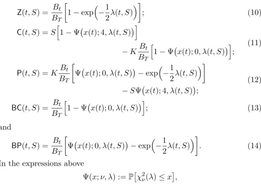
Figure 4 displays the results for the zero-coupon bond. The top left panel compares the evolution of the real-world bond price Z(t, S_t) with that of the standard bond price Bt/BT, which is obtained by discounting the

bond’s principal at the risk-free rate. As demonstrated in (9), the real-world price corresponds to the value of the cheapest hedge, and we observe that Z(t, St)≤Bt/BT, as is obvious from (10). Also, the real-world price is

initially quite sensitive to index fluctuations, while the standard price follows a smooth trajectory. The reason for this is clear from the top right panel, which plots the proportion of the hedge portfolio invested in the index: Initially the hedge consists almost entirely of an index holding, which is gradually switched into the savings account, leading to full investment in the savings account around 10 years before the bond matures. The bottom panel in Figure 4 plots the evolution of the benchmarked hedge error (i.e. the

7_{Note that since there is no record of instruments with such extreme maturities trading}

in the market, it was impossible to calibrate the model to observed derivative prices, as is usually done in empirical studies hedge performance.

(14)

benchmarked difference between the real-world bond price and the value of the hedge portfolio) over time. We argue that since the index is the natural unit of value in our approach, this graph provides a reliable picture of the performance of the hedge.

0 10 20 30 40 50 60 70 80 90 0 0.1 0.2 0.3 0.4 0.5 0.6 0.7 0.8 0.9 1 Zero−Coupon Bond Time Price 0 10 20 30 40 50 60 70 80 90 0 0.1 0.2 0.3 0.4 0.5 0.6 0.7 0.8 0.9 1 Hedge Portfolio Time Index Proportion 0 10 20 30 40 50 60 70 80 90 −1.5 −1 −0.5 0 0.5 1 1.5 2 2.5 3x 10 −5 _{Hedge Performance} Time

Benchmarked Hedge Error

Figure 4. Hedge simulation results for the zero-coupon bond: (top left) the evolution of real-world and standard bond prices over time; (top right) the proportion of the hedge portfolio invested in the index; and (bottom) the bench-marked hedge error.

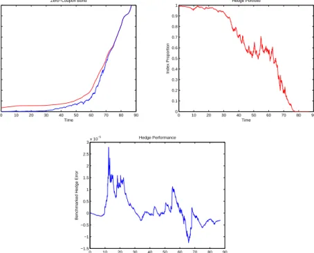
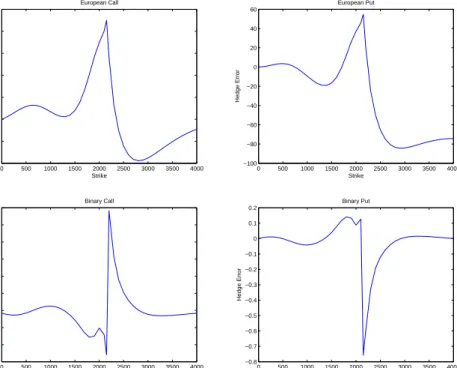
Figure 5 plots the terminal hedge errors for European calls and puts, and binary calls and puts, against strike. The hedge performance appears to be quite good everywhere except for strikes that are close to the final index value. This, however, is a natural consequence of the large negative gamma of at-the-money options, exascerbated in our case by infrequent delta hedging. Figure 6 refines the picture, by plotting terminal hedge error against strike for all four options. Again we observe prominent “gamma spikes” for close-to-the-money strikes, as well as a certain periodicity of the error, both of which are established stylized features of discrete hedging, and not necessarily indicative of model misspecification.

(15)

0 500 1000 1500 2000 2500 3000 3500 4000 −500 0 500 1000 1500 2000 2500 European Call Strike Payoff 0 500 1000 1500 2000 2500 3000 3500 4000 −500 0 500 1000 1500 2000 European Put Strike Payoff 0 500 1000 1500 2000 2500 3000 3500 4000 −0.2 0 0.2 0.4 0.6 0.8 1 1.2 Binary Call Strike Payoff 0 500 1000 1500 2000 2500 3000 3500 4000 −0.2 0 0.2 0.4 0.6 0.8 1 1.2 Binary Put Strike Payoff

Figure 5. Option payoffs and terminal hedge portfolio val-ues for (top left) European calls; (top right) European puts; (bottom left) binary calls; and (bottom right) binary puts.

6. Conclusions

Risk-neutral pricing in continuous-time financial markets relies on the rather austere NFLVR condition of Delbaen and Schachermayer [13] for its economic justification. A sequence of recent papers [see e.g. 27, 28, 33, 39] has questioned the economic necessity of this condition, and a consensus appears to be emerging that a theoretically sound market model need only conform to a much weaker no-arbitrage requirement. The effect of this is added modelling freedom, which we exploit to model a market containing a diversified equity accumulation index and a risk-free savings account.

Although our model does not accommodate an equivalent risk-neutral probability measure, it nevertheless satisfies the weak no-arbitrage condition alluded to above. Furthermore, we demonstrate that contingent claims on the index can be priced and hedged with this model, since all self-financing portfolios denominated in units of the index are local martingales under the real-world probability measure. In other words, martingale pricing can be applied, with the index as num´eraire asset and the real-world probability measure as pricing measure. Using this approach, we derive convenient expressions for the prices and hedge ratios of a number of standard European claims. Their effectiveness is demonstrated with a series of extremely long-term hedge simulations, using monthly historical data.

Our ambitions in this paper are two-fold: Firstly, while the articles cited above are generally concerned with fairly abstract economic consequences of relaxing the NFLVR requirement, we wish to demonstrate concretely that

(16)

0 500 1000 1500 2000 2500 3000 3500 4000 −40 −20 0 20 40 60 80 100 European Call Strike Hedge Error 0 500 1000 1500 2000 2500 3000 3500 4000 −100 −80 −60 −40 −20 0 20 40 60 European Put Strike Hedge Error 0 500 1000 1500 2000 2500 3000 3500 4000 −0.3 −0.2 −0.1 0 0.1 0.2 0.3 0.4 0.5 0.6 Binary Call Strike Hedge Error 0 500 1000 1500 2000 2500 3000 3500 4000 −0.8 −0.7 −0.6 −0.5 −0.4 −0.3 −0.2 −0.1 0 0.1 0.2 Binary Put Strike Hedge Error

Figure 6. Terminal hedge errors for (top left) European calls; (top right) European puts; (bottom left) binary calls; and (bottom right) binary puts.

pricing and hedging can be achieved in a market without an equivalent risk-neutral probability measure. In other words, from a practical point of view, eschewing the risk-neutral approach does not necessarily present as many difficulties as one might expect. In this context, the MMM should be regarded as an illustrative tool: Although we believe it exhibits many features of a good equity accumulation index model, there is an on-going effort to develop a model of greater verisimilitude. Secondly, we hope the reader will find the outcomes of the empirical hedge experiments sufficiently promising to justify further consideration. In this regard, we have focussed especially on extreme maturity contracts, since anecdotal evidence suggests risk-neutral pricing and hedging are not overly successful in this setting.

Appendix A. Squared Bessel Processes

A squared Bessel process Xδ _{= (}_Xδ

t)t≥0 of dimension δ ≥ 0 [see 35,

Chap. XI] is a solution to the SDE

dX_tδ =δ dt+ 2

q Xδ

t dWt,

with Xδ

0 =x > 0. A fundamental question is whether or not Xδ can ever

reach the origin. The answer depends the value of δ. In detail, let

ζδ := inf©t >0 : X_tδ= 0ª

(17)

be the first-passage time to zero for Xδ_{. We then obtain the following [see} 35, Chap. XI]: P£ζδ <∞¯¯X₀δ=x¤= ( 1 if 0≤δ <1 0 ifδ ≥2, while P£ζδ _<_∞¯¯_Xδ 0 =x ¤ ∈(0,1) if 1≤δ <2.

Assuming the origin can be reached (i.e. 0 ≤δ <2), another important question concerns the behaviour of the process there. Feller’s boundary clas-sification [see e.g. 8, Chap. II.6] reveals that the origin is exit-not-entrance if δ= 0, and non-singular if 0< δ <2. In the former case, the origin is ab-sorbing, while in the latter case the behaviour of Xδ _{at zero is not uniquely}

determined, and must be specified. Following Revuz and Yor [35], Chap. XI, we prescribe instantaneous reflection at the origin, for δ∈(0,2).

With its boundary behaviour at the origin specified, the transition density of Xδ_{, for}_{δ >}_{0, is given by [see 35, Chap. XI]}

qδ(t, x, y) =    1 2texp ¡ −x₂+_ty¢¡y_x¢δ−42_I_δ₋₂ 2 ³√_xy t ´ ifx >0 1 2tΓ(δ/2) ¡_y 2t ¢δ−2 2 _exp¡₋y 2t ¢ ifx= 0. (26)

Here I_µ(·) denotes the modified Bessel function of the first kind of order µ

[see e.g. 1, Chap. 9–10]. Since X0 _{is absorbed at zero, its distribution at}

any time comprises a discrete component that places a non-zero mass at the origin, as well as a continuous part. The former is the probability of absorption having already occurred, while the latter is the distribution of the process, conditional on it not having been absorbed yet. In detail, we have [see 35, Chap. XI]

P£X_t0 ≤z¯¯X₀0 =x] =P£ζ0≤t¯¯X₀0 =x¤+P£X_t0≤z¯¯ζ0 > t, X₀0 =x] = exp ³ −x 2t ´ + Z _z 0 q0(t, x, y)dy, (27)

where q0(t, x, y) is obtained by setting δ = 0 in (26), and recalling the identity I−1(·) =I1(·).

Our next topic is an absolute continuity relation due to Yor [43], Eq. 2.(c). Let δ ∈[0,2), and suppose the function g(·) satisfies the integrability con-dition lim x&0E ·_¡ X_t4−δ¢δ−22_g¡_X4−δ t ¢¯¯ ¯ ¯X04−δ=x ¸ <∞.

It can then be shown that

E h g¡X_tδ)I_{_ζδ_>t_} ¯ ¯ ¯X₀δ=x i =E "µ x X_t4−δ ¶2−δ 2 g¡X_t4−δ¢ ¯ ¯ ¯ ¯X04−δ=x # . (28) In particular, this establishes a correspondence between squared Bessel pro-cess of dimensions four and zero. In detail, taking δ= 0 in (28), we obtain

E h g¡X_t0¢ ¯¯¯X₀0=x i −g(0) exp ³ −x 2t ´ =E · x X4 t g¡X_t4¢ ¯ ¯ ¯ ¯X04=x ¸ , (29)

(18)

from (27). This device is used repeatedly in the derivations of the pricing formulae (10)–(14).

We now turn our attention to the relationship between squared Bessel processes and the non-central chi-square distribution. Let χ2

ν(λ) denote a

non-central chi-square random variable with ν ≥0 degrees of freedom and non-centrality parameter λ ≥ 0 [see 23, Chap. 29]. If λ = 0, it has an ordinary (central) chi-square distribution [see 22, Chap. 18], and we denote it by χ2

ν. In the case where ν > 0, the probability density function (PDF)

of χ2 ν(λ) is given by p(x;ν, λ) =    1 2e− λ+x 2 ³ x λ ´ν−2 4 Iν−2 2 ¡√ λx¢ ifλ >0 1 2Γ(ν/2) ¡_x 2 ¢ν−2 2 _exp¡₋x 2 ¢ ifλ= 0. (30) The distribution of the non-central chi-square variable χ2

0(λ) with zero

de-grees of freedom is given by [see 40]

P£χ2₀(λ)≤x¤=P£χ2₀(λ) = 0¤+P£0< χ2₀(λ)≤x¤ = exp ³ −λ 2 ´ + Z _x 0 p(ξ; 0, λ)dξ, (31)

wherep(x; 0, λ) is obtained by settingν = 0 in (30). As was the case for the distribution of the squared Bessel process with zero degrees of freedom, we see that the distribution of χ2

0(λ) contains a discrete component, placing a

mass at zero, and a continuous part. In fact, by comparing (26) with (30), and (27) with (31), we observe the following distributional equivalence:

Xδ t t (d) =χ2_δ ³_x t ´ , (32)

for all t > 0. This is the reason for the appearance of the non-central chi-square cumulative distribution function (CDF) throughout (11)–(14).

Finally, we briefly describe a scheme for simulating squared Bessel pro-cesses of integer dimension. Let δ ∈ N, and suppose W_i = (W_i,t)_t_≥₀, for

i = 1, . . . , δ, are independent Brownian motions satisfying Pδ_i₌₁W_i,2₀ = x. Using Itˆo’s formula, it is then easily shown that, conditional on Xδ

0 =x, X_tδ (d)= δ X i=1 W_i,t2. (33)

This means that squared Bessel processes of integer dimension can be sim-ulated exactly, by sampling independent Brownian motions.

Appendix B. Proof of Proposition 3

Proof. Firstly, (8) is well-defined, since the fact thathis not identically zero implies thatVh₍_{t, S}

t)>0. It is also clear thatSπ

h

0 =V0h. The Feynman-Kac

formula [see e.g. 34, p. 357] then yields

LVˆh(t, S) = 0, where ˆ Vh(t, S) :=E · h(ST) ST ¯ ¯ ¯ ¯St=S ¸ , 17

(19)

and the operatorL is defined by LG(t, S) := ∂G ∂t(t, S) + ¡ r(t) +θ2(t, S)¢S∂G ∂S(t, S) + 1 2θ 2₍_{t, S}₎_S2∂2G ∂S2(t, S).

Since Vh(t, S) =SVˆh(t, S), we thus obtain

LVh(t, S) =SLVˆh(t, S) +¡r(t) +θ2(t, S)¢SVˆh(t, S) +θ2(t, S)S2∂Vˆh ∂S (t, S) =¡r(t) +θ2(t, S)¢Vh(t, S) +θ2(t, S)S · ∂Vh ∂S (t, S)− 1 SV h₍_{t, S}₎ ¸ =r(t)Vh(t, S) +θ2(t, S)S∂Vh ∂S (t, S).

Finally, combining the above with Itˆo’s formula and (8) gives

dVh(t, St) = ∂V h ∂t (t, St)dt+ ∂Vh ∂S (t, St)dSt+ 1 2 ∂2_Vh ∂S2 (t, St)dhSit =LVh(t, St)dt+θ(t, St)St∂V h ∂S (t, St)dWt =¡r(t) +θ2(t, St)πh(t, St) ¢ Vh(t, St)dt+θ(t, St)πh(t, St)Vh(t, St)dWt.

We thus conclude from (5) thatSπh =Vh. ¤

Appendix C. Derivations of Pricing Formulae

Using (3), we may express the pricing function Vh₍_·_,_·_{) in (7) as follows:}

Vh(t, S) =SE · h(ST) ST ¯ ¯ ¯ ¯St=S ¸ =SE " h¡BTXϕ(T) ¢ BTXϕ(T) ¯ ¯ ¯ ¯ ¯Xϕ(t)=S/Bt # . (34) Note that X = X4 _{in (34) is a squared Bessel process of dimension four}8_.

Next, from (32) we obtain

X_ϕ₍_T₎(d)= ∆ϕ(t)χ2₄¡λ(t, S)¢, (35) conditional on X_ϕ₍_t₎=S/Bt. Here λ(t, S) and ∆ϕ(t) are given by (15) and

(16), respectively. In this way (34) may be expressed as the expected value of a function of a chi-square random variable with four degrees of freedom. Finally, observe that the identity

E · λ(t, S) χ2 4 ¡ λ(t, S)¢g ³ χ2₄¡λ(t, S)¢´ ¸ =E h g ³ χ2₀¡λ(t, S)¢´i−g(0) exp µ −λ(t, S) 2 ¶ , (36)

for an appropriately integrable functiong(·), results from using (35) to trans-late (29) into the language of non-central chi-square variables.

(20)

We now apply (34)–(36) to derive the real-world prices the claims listed in Table 1, starting with the zero-coupon bond:

Z(t, S) =SE · 1 ST ¯ ¯ ¯ ¯St=S ¸ =SE " 1 BTXϕ(T) ¯ ¯ ¯ ¯ ¯Xϕ(t)=S/Bt # =SE " 1 BT∆ϕ(t)χ2₄ ¡ λ(t, S)¢ # = Bt B_TE " λ(t, S) χ2 4 ¡ λ(t, S)¢ # = Bt BT · 1−exp ³ −1 2λ(t, S) ´¸ .

Note that the final equality above is an instance of (36), with g(ξ) := 1. Next, we price the European call, as follows:

C(t, S) =SE · (ST −K)+ S_T ¯ ¯ ¯ ¯St=S ¸ =SE · I© BTXϕ(T)>K ª ¯ ¯ ¯ ¯Xϕ(t)=S/Bt ¸ −KSE " I© BTXϕ(T)>K ª 1 BTXϕ(T) ¯ ¯ ¯ ¯ ¯Xϕ(t)=S/Bt # =SE · I© χ2 4 ¡ λ(t,S)¢>x(t)ª ¸ −KBt BTE " I© χ2 4 ¡ λ(t,S)¢>x(t)ª λ(t, S) χ2 4 ¡ λ(t, S)¢ # =SP h χ2₄¡λ(t, S)¢> x(t) i −KBt BTP h χ2₀¡λ(t, S)¢> x(t) i =S h 1−Ψ¡x(t); 4, λ(t, S)¢i−KBt B_T h 1−Ψ¡x(t); 0, λ(t, S)¢i,

where x(t) is given by (15). Note that the second-last equality above is again an application of (36), with g(ξ) := I_{_ξ>x₍_t₎_}, so that g(0) = 0. We now derive the price of the European put:

P(t, S) =SE · (K−S_T)+ ST ¯ ¯ ¯ ¯St=S ¸ =KSE " I© BTXϕ(T)≤K ª 1 B_TX_ϕ₍_T₎ ¯ ¯ ¯ ¯ ¯Xϕ(t)=S/Bt # −SE · I© BTXϕ(T)≤K ª ¯ ¯ ¯ ¯Xϕ(t)=S/Bt ¸ =KBt B_TE " I© χ2 4 ¡ λ(t,S)¢≤x(t)ª λ(t, S) χ2 4 ¡ λ(t, S)¢ # −SE · I© χ2 4 ¡ λ(t,S)¢≤x(t)ª ¸ =KBt BT · P h χ2₀¡λ(t, S)¢≤x(t) i −exp ³ −1 2λ(t, S) ´¸ −SP h χ2₄¡λ(t, S)¢≤x(t) i =KBt B_T · Ψ¡x(t); 0, λ(t, S)¢−exp ³ −1 2λ(t, S) ´¸ −SΨ¡x(t); 4, λ(t, S)¢. 19

(21)

For the second-last equality above, we use (36) with g(ξ) :=I_{_ξ_≤_x₍_t₎_}, from which it follows that g(0) = 1. To derive the pricing formula for the Euro-pean binary call, we proceed as follows:

BC(t, S) =SE · I_{_S_T_>K_} 1 S_T ¯ ¯ ¯ ¯St=S ¸ =SE " I© BTXϕ(T)>K ª 1 BTXϕ(T) ¯ ¯ ¯ ¯ ¯Xϕ(t) =S/Bt # = Bt B_TE " I© χ2 4 ¡ λ(t,S)¢>x(t)ª λ(t, S) χ2 4 ¡ λ(t, S)¢ # = Bt B_TP h χ2₀¡λ(t, S)¢> x(t) i = Bt B_T h 1−Ψ¡x(t); 0, λ(t, S)¢i.

Once again, the second-last equality follows from (36), withg(ξ) :=I_{_ξ>x₍_t₎_}. Finally, for the price of the European binary put, we obtain

BP(t, S) =SE · I_{_S_T_≤_K_} 1 ST ¯ ¯ ¯ ¯St=S ¸ =SE " I© BTXϕ(T)≤K ª 1 BTXϕ(T) ¯ ¯ ¯ ¯ ¯Xϕ(t) =S/Bt # = Bt BTE " I© χ2 4 ¡ λ(t,S)¢≤x(t)ª λ(t, S) χ2 4 ¡ λ(t, S)¢ # = Bt BT · P h χ2₀¡λ(t, S)¢≤x(t) i −exp ³ −1 2λ(t, S) ´¸ = Bt B_T · Ψ¡x(t); 0, λ(t, S)¢−exp ³ −1 2λ(t, S) ´¸ .

As before, the second-last equality is an application of (36) with g(ξ) :=

I_{_ξ_≤_x₍_t₎_}.

References

[1] M. Abramowitz and I. A. Stegun, editors. Handbook of Mathematical Functions With Formulas, Graphs, and Mathematical Tables. Dover, 1972.

[2] Y. A¨ıt-Sahalia. Maximum likelihood estimation of discretely sampled diffusions: A closed-form approximation approach. Econometrica, 70 (1):223–262, 2002.

[3] L. B. G. Andersen and V. V. Piterbarg. Moment explosions in stochastic volatility models. Finance Stoch., 11(1):29–50, 2007.

[4] O. E. Barndorff-Nielsen. Processes of normal inverse Gaussian type.

Finance Stoch., 2(1):41–68, 1998.

[5] D. S. Bates. Jumps and stochastic volatility: Exchange rate processes implicit in Deutsche mark options. Rev. Finan. Stud., 9(1):69–107, 1996.

(22)

[6] F. Black. Studies in stock price volatility changes. InProceedings of the 1976 Business Meeting of the Business and Economic Statistics Section, pages 177–181. American Statistical Association, 1976.

[7] F. Black and M. Scholes. The pricing of options and corporate liabilities.

The Journal of Political Economy, 81(3):637–654, 1973.

[8] A. N. Borodin and P. Salminen.Handbook of Brownian Motion — Facts and Formulae. Probability and Its Applications. Birkh¨auser Verlag, Basel, second edition, 2002.

[9] P. Carr, H. Geman, D. B. Madan, and M. Yor. The fine structure of asset returns: An empirical investigation. J. Bus., 75(2):305–332, 2002. [10] P. Carr, H. Geman, D. B. Madan, and M. Yor. Stochastic volatility for

L´evy processes. Math. Finance, 13(3):345–382, 2003.

[11] A. M. G. Cox and D. G. Hobson. Local martingales, bubbles and option prices. Finance Stoch., 9(4):477–492, 2005.

[12] J. C. Cox and S. A. Ross. The valuation of options for alternative stochastic processes. J. Finan. Econ., 3(1–2):145–166, 1976.

[13] F. Delbaen and W. Schachermayer. A general version of the fundamen-tal theorem of asset pricing. Math. Ann., 300(3):463–520, 1994. [14] D. Duffie, J. Pan, and K. Singleton. Transform analysis and asset

pricing for affine jump-diffusions.Econometrica, 68(6):1343–1376, 2000. [15] G. B. Durham and A. R. Gallant. Numerical techniques for maximum likelihood estimation of continuous-time diffusion processes. J. Bus. Econ. Statist., 20(3):297–316, 2002.

[16] P. H. Dybvig and C. Huang. Non-negative wealth, absence of arbitrage, and feasible consumption plans. Rev. Finan. Stud., 1(4):377–401, 1988. [17] E. Eberlein, U. Keller, and K. Prause. New insights into smile, mispric-ing and value at risk: The hyperbolic model. J. Bus., 71(3):371–405, 1998.

[18] H. Geman, N. El Karoui, and J.-C. Rochet. Changes of num´eraire, changes of probability measure and option pricing. J. Appl. Probab., 32 (2):443–458, 1995.

[19] S. L. Heston. A closed-form solution for options with stochastic volatil-ity with applications to bond and currency options. Rev. Finan. Stud., 6(2):327–343, 1993.

[20] S. L. Heston, M. Loewenstein, and G. A. Willard. Options and bubbles.

Rev. Finan. Stud., 20(2):359–389, 2007.

[21] J. Hull and A. White. The pricing of options on assets with stochastic volatilities. J. Finance, 42(2):281–300, 1987.

[22] N. L. Johnson, S. Kotz, and N. Balakrishnan. Continuous Univariate Distributions: Volume 1. Wiley Series in Probability and Mathematical Statistics. John Wiley & Sons, New York, second edition, 1994.

[23] N. L. Johnson, S. Kotz, and N. Balakrishnan. Continuous Univariate Distributions: Volume 2. Wiley Series in Probability and Mathematical Statistics. John Wiley & Sons, New York, second edition, 1995.

[24] S. G. Kou. A jump-diffusion model for option pricing. Management Sci., 48(8):1086–1101, 2002.

[25] D. Kramkov and W. Schachermayer. The asymptotic elasticity of utility functions and optimal investment in incomplete markets. Ann. Appl.

(23)

Probab., 9(3):904–950, 1999.

[26] R. S. Lipster and A. N. Shiryaev. Statistics of Random Processes, I. General Theory, volume 5 of Applications of Mathematics (Stochastic Modelling and Applied Probability). Springer-Verlag, Berlin, second edi-tion, 2001.

[27] J. Liu and F. A. Longstaff. Losing money on arbitrage: Optimal dy-namic portfolio choice in markets with arbitrage opportunities. Rev. Finan. Stud., 17(3):611–641, 2004.

[28] M. Loewenstein and G. A. Willard. Local martingales, arbitrage, and viability: Free snacks and cheap thrills. Econ. Theory, 16(1):135–161, 2000.

[29] R. Lowenstein. When Genius Failed: The Rise and Fall of Long-Term Capital Management. Random House, 2000.

[30] D. B. Madan and E. Seneta. The variance gamma (V.G.) model for share market returns. J. Bus., 63(4):511–524, 1990.

[31] R. C. Merton. Option pricing when underlying stock returns are dis-continuous. J. Finan. Econ., 3(1–2):125–144, 1976.

[32] E. Platen. A minimal financial market model. InMathematical Finance (Konstanz, 2000), Trends in Mathematics, pages 293–301. Birkh¨auser, Basel, 2001.

[33] E. Platen. Arbitrage in continuous complete markets. Adv. in Appl. Probab., 34(3):540–558, 2002.

[34] E. Platen and D. Heath. A Benchmark Approach to Quantitative Fi-nance. Springer Finance. Springer-Verlag, Berlin, 2006.

[35] D. Revuz and M. Yor. Continuous Martingales and Brownian Mo-tion, volume 293 of Grundlehren der mathematischen Wissenschaften. Springer-Verlag, Berlin, third edition, 1999.

[36] L. C. G. Rogers and D. Williams. Diffusions, Markov Processes and Martingales, Volume 2: Itˆo Calculus. Cambridge Mathematical Library. Cambridge University Press, Cambridge, second edition, 2000.

[37] M. Schroder. Computing the constant elasticity of variance option pric-ing formula. J. Finance, 44(1):211–219, 1989.

[38] D. Schutz. Der Fall der UBS. Bilanz, 2000.

[39] A. Shleifer and R. W. Vishny. The limits of arbitrage. J. Finance, 52 (1):35–55, 1997.

[40] A. F. Siegel. The noncentral chi-squared distribution with zero degrees of freedom and testing for uniformity. Biometrika, 66(2):381–386, 1979. [41] C. A. Sin. Complications with stochastic volatility models. Adv. in

Appl. Probab., 30(1):256–268, 1998.

[42] E. M. Stein and J. C. Stein. Stock price distributions with stochastic volatility: An analytic approach.Rev. Finan. Stud., 4(4):727–752, 1991. [43] M. Yor. On some exponential functionals of Brownian motion. Adv. in

(24)

Eckhard Platen, School of Finance and Economics & Department of Math-ematical Sciences, University of Technology, Sydney, P.O. Box 123, Broad-way, NSW 2007, Australia

E-mail address: [email protected]

Hardy Hulley, School of Finance and Economics, University of Technol-ogy, Sydney, P.O. Box 123, Broadway, NSW 2007, Australia

E-mail address: [email protected]