2009
A study of time-decayed aggregates computation
on data streams
Bojian Xu
Iowa State UniversityFollow this and additional works at:
https://lib.dr.iastate.edu/etd
Part of the
Electrical and Computer Engineering Commons
This Dissertation is brought to you for free and open access by the Iowa State University Capstones, Theses and Dissertations at Iowa State University Digital Repository. It has been accepted for inclusion in Graduate Theses and Dissertations by an authorized administrator of Iowa State University Digital Repository. For more information, please [email protected].
Recommended Citation
Xu, Bojian, "A study of time-decayed aggregates computation on data streams" (2009).Graduate Theses and Dissertations. 10956. https://lib.dr.iastate.edu/etd/10956
by Bojian Xu
A dissertation submitted to the graduate faculty in partial fulfillment of the requirements for the degree of
DOCTOR OF PHILOSOPHY
Major: Computer Engineering Program of Study Committee: Srikanta Tirthapura, Major Professor
Pavan Aduri Soma Chaudhuri
Daji Qiao Zhao Zhang
Iowa State University Ames, Iowa
2009
TABLE OF CONTENTS
LIST OF FIGURES . . . . v
ACKNOWLEDGEMENTS . . . . vi
ABSTRACT . . . . vii
CHAPTER1. Introduction . . . . 1
1.1 Asynchronous Data Streams . . . 2
1.2 Distributed Data Streams Processing Diagram . . . 3
1.3 Data Stream Model . . . 4
1.4 Time Decay . . . 5
1.4.1 Decomposable Decay Functions . . . 5
1.5 Thesis Contributions . . . 6
1.6 Roadmap . . . 8
1.7 Declarations . . . 8
CHAPTER2. Sliding Windows Decay Based Processing . . . . 10
2.1 Introduction . . . 10
2.1.1 Contributions . . . 11
2.1.2 Related Work . . . 14
2.2 Sum of Positive Integers . . . 17
2.2.1 Intuition . . . 17
2.2.2 Formal Description of the Algorithm . . . 19
2.2.3 Correctness Proof. . . 19
2.2.4 Complexity . . . 27
2.2.5 Trade off between Processing time and Query time. . . 28
2.3 Computing the Median . . . 29
2.3.1 Formal Description of the Algorithm . . . 30
2.3.2 Correctness Proof. . . 31
2.3.3 Complexity . . . 37
2.4 Union of Sketches . . . 37
CHAPTER3. General Time-decay Based Processing . . . . 43 3.1 Introduction . . . 43 3.1.1 Problem Formulation . . . 45 3.1.2 Aggregates . . . 45 3.1.3 Contribution . . . 47 3.2 Related Work . . . 48
3.3 Aggregates over an Integral Decay Function . . . 51
3.3.1 High-level description . . . 51
3.3.2 Formal Description . . . 54
3.3.3 Computation of Expiry Time . . . 57
3.3.4 Computing Decayed Aggregates Using the Sketch . . . 65
3.4 Decomposable Decay Functions via Sliding Window . . . 73
3.4.1 Sliding Window Decay . . . 73
3.4.2 Reduction from a Decomposable Decay Function to Sliding Window Decay . . 74
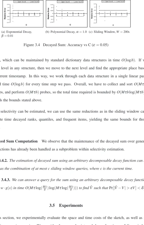
3.5 Experiments . . . 77
3.5.1 Experimental Setup. . . 80
3.5.2 Accuracy vs Space Usage . . . 81
3.5.3 Time Efficiency . . . 83
3.6 Concluding Remarks . . . 84
CHAPTER4. General Time-decay Based Correlated Processing . . . . 85
4.1 Introduction . . . 85 4.1.1 Problem Formulation . . . 87 4.1.2 Contributions . . . 88 4.2 Prior Work. . . 89 4.3 Upper Bounds . . . 90 4.3.1 Additive Error . . . 90 4.3.2 Relative Error . . . 92 4.4 Lower Bounds . . . 103 4.4.1 Finite Decay . . . 103 4.4.2 Exponential Decay . . . 104 4.4.3 Super-exponential Decay . . . 110
4.4.4 Finite (Super) Exponential Decay . . . 111
4.4.5 Sub-exponential decay . . . 111
4.5 Experiments . . . 112
4.6 Concluding Remarks . . . 114
CHAPTER5. Forward Decay: A Practical Decay Model for Stream Systems . . . 116
5.1 Introduction . . . 116
5.2.1 Backward Decay Functions . . . 119
5.3 Forward Decay . . . 120
5.3.1 Exponential Decay . . . 121
5.3.2 Polynomial Decay . . . 122
5.3.3 Landmark windows. . . 123
5.4 Aggregate Computation under Forward Decayed Models . . . 124
5.4.1 Count, Sum and Average . . . 124
5.4.2 Min and Max . . . 126
5.4.3 Heavy Hitters and Quantiles . . . 126
5.4.4 Count Distinct . . . 129
5.5 Sampling Under Forward Decay . . . 130
5.5.1 Sampling With Replacement . . . 130
5.5.2 Sampling Without Replacement . . . 131
5.5.3 Sampling Under Exponential Decay . . . 132
5.6 Implementing Forward Decay . . . 132
5.6.1 Numerical issues . . . 132
5.6.2 Out-of-order and Distributed arrivals. . . 133
5.7 Related Work on Time Decay . . . 133
5.8 Experimental Evaluation . . . 136 5.8.1 Experimental Results. . . 137 5.9 Concluding Remarks . . . 141 CHAPTER6. Conclusion . . . 142 6.1 Future Work . . . 143 BIBLIOGRAPHY . . . 145
LIST OF FIGURES
Figure 2.1 An example of distributed data stream aggregation. . . 38
Figure 3.1 An example of computing the time decayed sum . . . 54
Figure 3.2 Find fm∈F over the Ring of Z¯ ain the Case of r<a/2 . . . 63
Figure 3.3 Reduction of a decomposable decay function to sliding window. . . 74
Figure 3.4 Experiments on decayed sum . . . 77
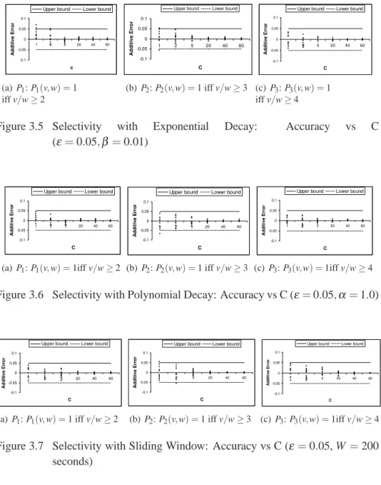
Figure 3.5 Experiments on selectivity over exponential decay . . . 78
Figure 3.6 Experiments on selectivity over polynomial decay . . . 78
Figure 3.7 Experiments on selectivity over sliding window . . . 78
Figure 3.8 Experiments on sketch size . . . 78
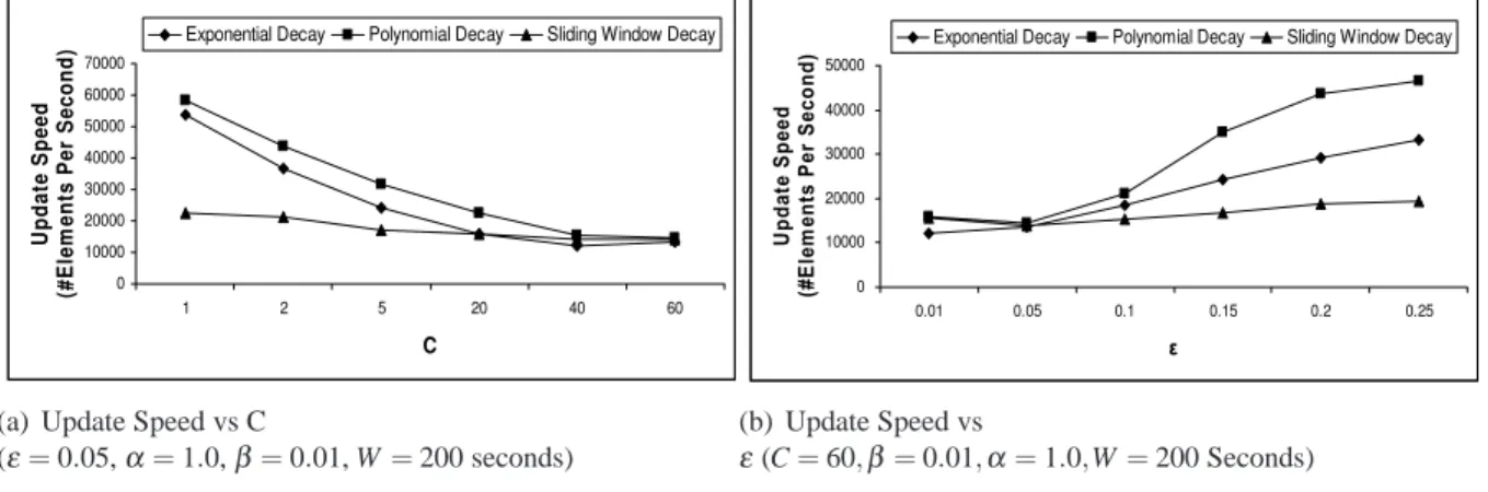
Figure 3.9 Experiments on sketch update speed: different decay functions . . . 79
Figure 3.10 Experiments on sketch update speed: different decay speeds . . . 79
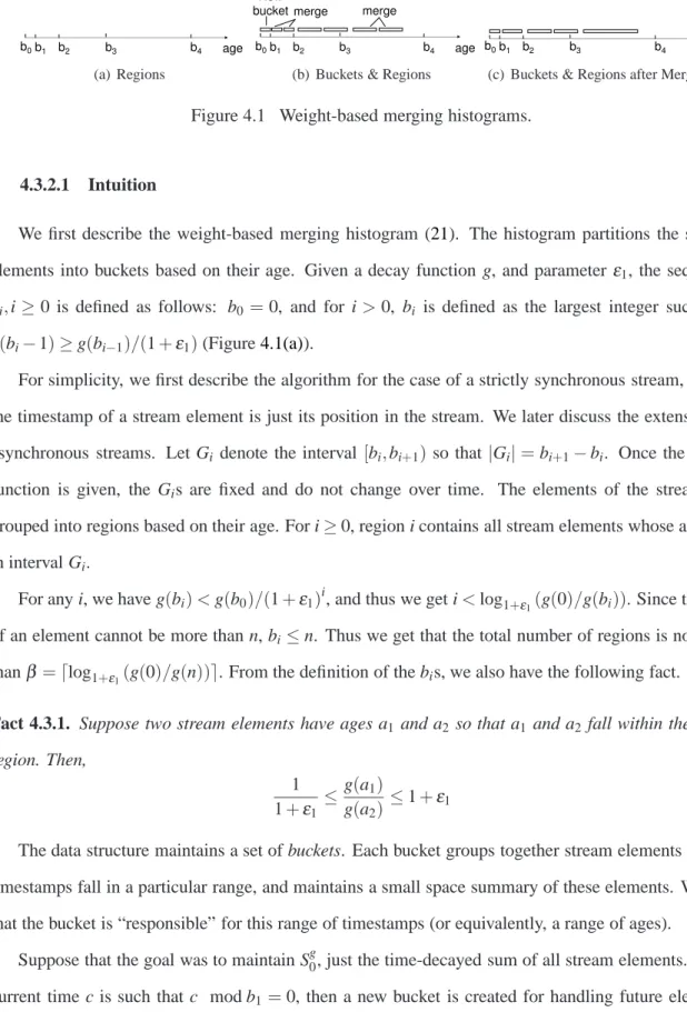
Figure 4.1 Weight-based merging histograms. . . 93
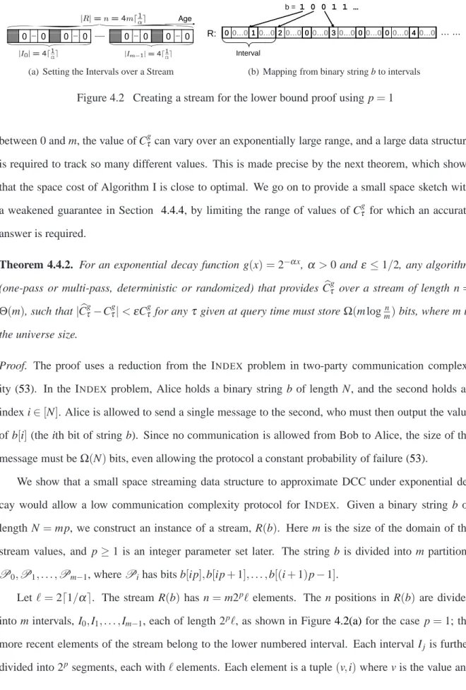
Figure 4.2 A stream for exponential decay based DCS’s lower bound proof . . . 106
Figure 4.3 Experiments on sliding window based DCS . . . 112
Figure 4.4 Experiments on the throughput of relative error guaranteed algorithm . . . 113
Figure 5.1 Relative decay property for the monomial decay functions . . . 122
Figure 5.2 Experiments on Count queries under time decay . . . 134
Figure 5.3 Experiments on Sampling Queries under time decay . . . 137
Figure 5.4 Experiments on Heavy Hitter queries under time decay . . . 139
ACKNOWLEDGEMENTS
First and most, I want to thank my advisor Srikanta Tirthapura for leading me into the area and giving me so much freedom in doing research. His standard for quality work and enormous patience for new discoveries make my doctoral study an enjoyable experience. His generous support also enables me to be focused on my study. Graham Cormode was an excellent mentor when I visited AT&T as an intern in Summer 2008. I want to thank him for his research discussion and collaboration since then. I want to thank Costas Busch, Vladislav Shkapenyuk and Divesh Srivastava for their research contributions in this work. I also want to thank Chris Chu for being my advisor in the Preparing Future Faculty program. His being a good role model has often inspired me to be a better student and researcher. I also owe him for squeezing time from his busy schedule to review my job application documents. I would also like to thank my committee members, Dr. Pavan Aduri, Dr. Soma Chaudhuri, Dr. Daji Qiao and Dr. Zhao Zhang, for their advice in this work.
I want to thank my officemates, Tycho Anderson, Bibudh Lahiri, Puvi Pandian, Zhenhui Shen and Jason Stanek, for the research discussions and the fun in the river fishing together. I want to thank my roommates, Guanghai Ji, Rong Jiao, Scott Polifka, Song Sun and Kewei Tu, for their friendship. I also want to thank the brothers and sisters in Christ in TCCF and CEFCA, for their encouragement during my stay in US.
I want to appreciate my parents Qingyue Xu and Suqing Hong for their unconditional love. I will never have a chance to be who I am without their endless giving. I also want to thank my sisters Sili and Sijian and their families, who I have been missing so much all the time, for their being part of my loving family in China. Finally, I want to thank my wife, Weili, for her love and silent support, and more sweetness in the future.
Finally but not least, I want to thank the Almighty Lord, who I am still pursuing, for giving me the purpose and strength to keep growing. To him be all the glory.
ABSTRACT
Many real world data naturally arrive as rapid paced and virtually unbounded streams. Examples of such streams include network traffic at a router, events observed by a sensor network, accesses to a web server and transactional updates to a large database. Such streaming data need to be monitored online to collect traffic statistics, detect trends and anomalies, tune system performance and help make business decisions. However, because of the large size and rapid pace of the data, as well as the online processing requirement, conventional data processing methods, such as storing the data in a database and issuing offline SQL queries thereafter, are not feasible. Data stream processing is a new diagram of massive data set processing and creates new challenges in the algorithm design and implementation. In this thesis, we consider time-decayed data aggregation for data streams, where the importance or contribution of each data element decays over time, since recent data are usually considered of more importance in applications, and therefore are given heavier weights. We design small space data structures and algorithms for maintaining fundamental aggregates of the streams if it is possible and otherwise show large space lower bounds.We consider the data aggregation over a robust data stream model called asynchronous data stream, motivated by the streaming data transmitted in distributed systems, including computer networks, where the asynchrony in the data transmission is inevitable. In asynchronous data stream, the arrival order of the data elements at the receiver side is not necessarily the same as the order in which the data elements were generated. Asynchronous data stream is a robuster and generalized model of the previous synchronous data stream model.
In summary, this thesis presents the following results:
• We formalize the model of asynchronous data stream and the notion of timestamp sliding win-dow. We propose the first small space sketch for summarizing the data elements over timestamp sliding windows of multiple geographically distributed asynchronous data streams. The sketch can return accuracy guaranteed estimates for basic aggregates, such as: Sum, Median and
Quan-tiles.
• We design the first small space sketch for general purpose network streaming data aggregation. The sketch has the following properties that make it useful in communication-efficient aggre-gation in distributed streaming scenarios: (1) The sketch can handle multiple geographically distributed asynchronous data streams. (2) The sketch is duplicate-insensitive, i.e. reinsertions of the same data will not affect the sketch, and hence the estimates of aggregates. (3) The sketch is also time-decaying, so that the weight of each data element summarized in the sketch decreases over time. (4) The sketch returns accuracy guaranteed estimates for a variety of core aggregates, including the sum, median, quantiles, frequent elements and selectivity.
• We conduct a comprehensive study on the time-decayed correlated data aggregation over asyn-chronous data streams. For each class of time decay function, we either propose space efficient algorithms or show large space lower bounds. We not only closes the open problem of correlated data aggregation under sliding windows decay, but also presents negative results for the case of exponential decay, which however is highly used in the non-correlated scenarios.
• We propose the forward decay model to simplify the time-decayed data stream aggregation and sampling. Forward decay captures a variety of usual decay functions (or called backward decay), such as exponential decay. We design efficient algorithms for data aggregation and sampling under the forward decay model, and show that they are easy to implement scalably.
CHAPTER 1. Introduction
Many real world data naturally arrive as streams. Examples include network traffic at a router, events observed by the sensor motes of a wireless sensor network, webpage requests to a web server and transactional updates to a large database. Contributed by the advancement of modern computer and Internet technologies, such streaming data has became highly paced and massive, compared to the ability of computing, storing and transmitting that the data processor can provide. For example, an OC48 link has its standard transmission rate at 2.5 Gbits per second, much more than the storage capacity of a normal computer, and the flowing data are even too quick to take a scan of it; In the recently emerging wireless sensor network applications, events observed by the battery powered tiny sensor mote can quickly overwhelm the mote’s memory.
However, these streaming data need to be monitored to collect traffic statistics, detect trends and anomalies, tune system performance and even help make business decisions. In some applications, re-altime queries and answers are even demanded. For example, a search engine may want to continuously maintain a list of hot searching keywords mined from the massive streams of searching queries that the search engine has received from the users. However, because of the large size and rapid pace of the data as well as the demands for realtime queries and answers, conventional data processing methods, such as storing the data in a database and issuing offline SQL queries, are not feasible.
The goal in data stream processing research is to answer questions like: Given such amount of time and space, and a data steam or multiple streams arriving at such a pace, what query about the streams can we answer ? If not, can we give an approximate answer for the query ? How accurate the approximate answer can we guarantee ? Or can we show that the problem is inherently unsolvable in a streaming fashion using such limited space and time budget ? The typical challenges in the algorithms design and implementation for the data stream processing are as follows.
unbounded stream size, the space cost of the algorithm usually must be poly-logarithmic in the size of the streams and sometimes even independent from the stream size. A small workspace also help in processing stream elements more quickly by reducing the time cost in scanning and searching through the data structures.
2. The algorithm must process each stream element quickly in order to keep up with the pace of the stream.
3. Constrained by the small space budget, one-pass processing of the stream is required, since we are incapable to store the majority of the stream and therefore have no chance to visit old data elements. One-pass processing is also needed to support continuous queries.
4. Queries of interest can be submitted at anytime during the stream processing. Answers should be returned immediately regarding the data that have been received so far. Answers for the queries can comprise a new stream and can be the input of another stream processor.
5. In many scenarios, the sacrifice of fast processing and small workspace is to lose the accuracy in the answers for queries. Although approximate answers are acceptable in many applications, error in these approximations need to be well bounded.
1.1 Asynchronous Data Streams
In this thesis, we particularly focus on asynchronous data streams (Definition1.3.1), motivated by the data streams transmitted in distributed systems including networks. In distributed stream process-ing, it is necessary to deal with the inherent asynchrony in the network through which data is being transmitted. Nodes often have to process composite data streams that consist of interleaved data from multiple data sources. One consequence of the network asynchrony is that in such composite data streams, the arrival order of the stream elements is not necessarily the same as the order in which the elements were generated. We call such a data stream as an asynchronous data stream.
Asynchronous data streams are inevitable anytime two streams, say A and B, fuse with each other and the data processing has to be done on the stream formed by the interleaving of A and B. Even if individual streams A or B are not inherently asynchronous, when the streams are fused, the stream
could become asynchronous. For example, if the network delay in receiving stream B is greater than the delay in receiving elements in stream A, then the the stream processor may consistently observe elements with earlier timestamps from B after elements with more recent timestamps from A.
In asynchronous data streams the order of “recency” of the data may not be preserved. The notion of recency can be captured with the help of a timestamp associated with the stream element. The greater the timestamp of an element is, the more recent the element is. Asynchronous stream is a more natural model for data streams transmitted in distributed systems than the synchronous stream model, and it is therefore robuster for distributed data stream monitoring.
1.2 Distributed Data Streams Processing Diagram
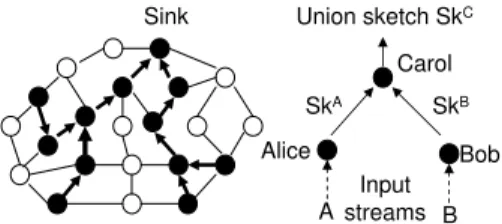
In applications involving distributed data sources, such as content distribution, intranet monitoring, and sensor data processing, no single node observes all data, yet aggregates should be computed over the union of the data observed at all the nodes. Therefore, it is necessary to answer aggregate queries for the union of all the streams distributively. A naive approach to solve such problems is to send all streams to a single aggregator. However, this approach is too costly, since there is a communication and energy cost for every data item in every stream. Thus, the data streams have to be combined in a more efficient way in order to minimize the use of network resources. This is critical especially in sensor networks where nodes are typically battery operated devices.
In our approach, we place an aggregator for each stream. Each aggregator maintains a small space
sketch summarizing its local stream. All the sketches for local streams can be combined distributively
to create the sketch for the union of streams (Figure 2.1). The sketch for the union can be used to answer queries regarding the union of streams. The sketches of local streams will be combined in a compact and lossless way, i.e., the space complexity and accuracy guarantee of the sketch for the union is the same as those for local streams. Also, the sketch for the union can be constructed on demand, whenever new queries are issued. Unlike previous work (42; 41; 57) that considered the synchronous model on distributed streams, this thesis considers aggregate computation over distributed streams under asynchronous arrival.
1.3 Data Stream Model
We model a stream as R=he1,e2, . . . ,eni, where eiis received earlier than ej for any pair of i and
j, i< j. Note that en is the most recently received element and n can be infinitely large. Each stream
element ei, 1≤i≤n, is a tuple(vi,wi,ti,idi), where the entries are defined as follows:
• viis a positive integer value
• wiis a weight associated with the value
• tiis the integer timestamp, tagged at the time eiwas created.
• idi is a unique id for ei.
This abstraction captures a wide variety of cases that can be encoded in this form. It is deliberately general; users can choose to assign values to these fields to suit their needs. For example, if the desired aggregate is the median temperature reading across all (distinct) observations, this can be achieved by setting all weights to wi=1 and the values vi to be actual temperatures observed. The unique
observation id idi can be formed as the concatenation of the unique sensor id and time of observation
(assuming there is only one reading per instant). We shall give more examples in Chapter3.
We consider asynchronous data stream. In other words, it is possible that in stream R an element tagged with a larger (and thus newer) timestamp is received earlier than an element of a smaller (and thus older) timestamp. More formally, we define an asynchronous data stream as follows.
Definition 1.3.1 (Asynchronous Data Stream). Stream R is an asynchronous data stream if for any pair of i and j, 1≤i< j≤n, it is possible that ti>tj.
Our stream model also allows the possibility that the same observation appears multiple times in the stream, with the same id, value, weight and timestamp preserved across multiple appearances. Such occurrences exist in real network environment due to the multi-path routing to increase the chance of data delivery, yet only one copy of such repeated occurrences should be considered while evaluating aggregates over the stream. Note that our model allows different elements of the stream to have different ids, but the same values, weights and/or timestamps — in such a case, they will be considered separately in computing the aggregates.
1.4 Time Decay
In most evolving settings, recent data is more reliable or more important than older data. We should therefore weigh newer stream elements (with larger timestamps) more heavily than older ones. This can be formalized in a variety of ways: we may only consider data elements that fall within a sliding
window of recent time (say, the last hour), and ignore (assign zero weight to) any that are older (35); or, more generally, use an arbitrary function that assigns a weight to each data element as a function of its initial weight and age (21).
The age of an element is defined as the elapsed time since the element was created. Thus, the age of element(v,w,t,id) at time c is c−t. A decay function takes the initial weight and the age of an
element and returns its decayed weight.
Definition 1.4.1. A decay function f(w,x)takes two parameters, the weight w≥0, and an integral age
x≥0, and should satisfy the following conditions. (1) f(w,x)≥0 for all w,x; (2) if w1>w2, then
f(w1,x)≥ f(w2,x); (3) if x1>x2, then f(w,x1)≤ f(w,x2).
The decayed weight of an element(v,w,t,id)at time c≥t is f(w,c−t). In Chapter5, we will also call such decay function as backward decay, since the value of it depends on the element’s age which is computed by looking from the current time backward to the element’s timestamp.
1.4.1 Decomposable Decay Functions
Decomposable decay is a class of decay functions and is popularly used in applications.
Definition 1.4.2. A decay function f(w,x)is a decomposable decay function if it can be written in the form f(w,x) =w·g(x)for some function g().
Note that the conditions on a decay function f(w,x)naturally impose the following conditions on
g(): (1) g(x)≥0 for all x; (2) if x1<x2, then g(x1)≥g(x2). In the rest of this thesis, we will also call
g(x)decay function if the context is clear. The following are example decomposable decay functions.
No decay. The trivial function g(x)≡1 weights all ages equally. This means that the time-decayed model captures prior work on non-decayed aggregates.
Sliding window. Given a “window size” parameter, W , the function g(x) =1 for x≤W and g(x) =0 for x>W captures the common sliding window semantics—only items whose age is less than or equal
to W are considered.
Polynomial decay. Given a constant a>0, the polynomial decay function is defined as g(x) = (x+1)−a.
Exponential decay. Given a constantα>0, the exponential decay function is defined as g(x) =2−αx. Exponential decay with a different base can also be written in this form, since a−λx=2−λlog2(a)x.
Super-exponential decay. A decay function g(x)is super-exponential, if there exist constantsσ >1 and c≥0, such that for every x≥c, f(x)/f(x+1)≥σ. Examples of such decay functions include: (1) polyexponential decay (21): g(x) = (x+1)k2−αx/k! where k>0, and α >0 are constants. (2)
g(x) =2−αxβ, whereα >0 andβ >1.
Converging decay. A decay function g(x) is a converging decay function if g(x+1)/g(x) is non-decreasing with x. Intuitively, the relative weights of elements with different timestamps under a converging decay function get closer to each other as time goes by. As pointed out by Cohen and Strauss (21), this is an intuitive property of a time-decay function in several applications. Many popular decay functions, such as exponential decay and polynomial decay, are converging decay. Converging decay also includes the no decay case: g(x)≡1.
Finite decay. A decay function is defined to be a finite decay function with age limit N, if there exists N≥0 such that for x>N, g(x) =0, and for x≤N, g(x)>0. Examples of finite decay include (1) sliding window decay, where the age limit N is the window size. (2) Chordal decay with an age limit
N−1 (21): g(x) =1−x/N if 0≤x≤N and g(x) =0 otherwise. Obviously, no finite decay function is a converging decay function, since g(N+1)/g(N) =0 while g(N)/g(N−1)>0.
1.5 Thesis Contributions
In this thesis, we focus on time-decayed asynchronous data stream processing. We design time and space efficient algorithms for data aggregations in the setting of distributed data streams. We also show large space lower bounds for problems that are inherently hard. The following are the main contributions of this thesis.
• We formalize the model of asynchronous data stream and the notion of timestamp sliding win-dow. We propose the first small space sketch for summarizing the data elements over timestamp sliding windows of multiple geographically distributed asynchronous data streams. The sketch can return accuracy guaranteed estimates for basic aggregates, such as: Sum, Median and Quan-tiles. (Chapter2)
• We propose the first small space sketch for general purpose network data aggregation. The sketch has the following properties that make it useful in communication-efficient aggregation in distributed streaming scenarios: (1) The sketch can handle asynchronous data streams. (2) The sketch is duplicate-insensitive, i.e. reinsertions of the same data will not affect the sketch, and hence the estimates of aggregates. (3) The sketch is also time-decaying, so that the weight of each data element summarized in the sketch decreases over time according to any arbitrary user-specified decay function. (4) The sketch can give provably approximate guarantees for a variety of core aggregates of data, including the sum, median, quantiles, frequent elements and selectivity. (5) The size of the sketch and the time taken to update it are both polylogarithmic in the size of the relevant data. (6) Multiple sketches computed over distributed data streams can be combined without loss of accuracy. (Chapter3)
• We conduct a comprehensive study on the time-decayed correlated data aggregation over asyn-chronous data streams. For each class of time decay function, we either propose space efficient algorithms or show large space lower bounds. We not only closes the open problem of correlated data aggregation under sliding windows decay, but also presents negative results for the case un-der exponential decay, which however is highly used in the non-correlated scenarios. (Chapter4)
• We propose the forward decay model to simplify the time-decayed data stream aggregation and sampling. Forward decay captures a variety of usual decay functions (or called backward decay), such as exponential decay and polynomial decay. We design efficient algorithms for data aggre-gation and sampling under the forward decay model, and show that they are easy to implement scalably. (Chapter5)
1.6 Roadmap
In Chapter 2, we consider asynchronous data stream processing over sliding windows and de-sign small space sketches for data aggregation. This sketch is further extended in Chapter3for more general purpose network streaming data aggregation. We then extend the techniques in processing asynchronous data stream for the correlated data stream aggregation in Chapter 4. In Chapter 5, we present forward decay, a new time decay model to simplify the time-decayed data stream aggregation and sampling. We conclude this thesis with several open problems in Chapter6.
1.7 Declarations
Publications. The work presented in this thesis has been published in the following computer science conference proceedings and journals. The majority of this thesis derives from these publications.
• The work of Chapter2has been published in (75) and (79).
• The work of Chapter3has been published in (30) and (32).
• The work of Chapter4has been published in (31) and (29).
• The work of Chapter5has been published in (28).
My Contributions. Like many thesis work, my thesis research is a collaborative work with my major professor Srikanta Tirthapura and other researchers from universities and research laboratories. Here I clarify my contributions in these collaborations.
• The proposal of the asynchronous data stream model, presented in Chapter2, is due to Srikanta Tirthapura. He also proposed the idea of sampling approach for solving the problem. I finished the technical proofs under his guidance.
• The proposal of designing a general purpose sketch for network streaming data aggregation, presented in Chapter3, is due to Srikanta Tirthapura and myself. The main algorithmic ideas and proofs for solving the problem as well as the experimental study are due to myself.
• The proposal of the time-decayed correlated data aggregation, presented in Chapter 4, is due to Srikanta Tirthapura and myself. Most of the algorithms and lower bound proofs are due to myself. Graham Cormode improved the space lower bound for the exponential decay based correlated sum based on my discovery of the lower bound and using my proof idea.
• The work presented in Chapter5was done during my visit to AT&T Shannon Laboratory as an intern in Summer 2008. The idea of forward decay is due to the colleagues at AT&T. I studied the sampling techniques under the forward decay model, as well as part of the experimental study.
CHAPTER 2. Sliding Windows Decay Based Processing
In this chapter, we study the problem of maintaining sketches for the data elements in the sliding windows over an asynchronous data stream. The sketches can give provably accurate estimates of two basic aggregates, the sum and the median, of the stream of numbers in the sliding windows. The space taken by the sketches, the time needed for querying the sketches, and the time for inserting new ele-ments into the sketches are all polylogarithmic with respect to the maximum window size. The sketches can be easily combined in a lossless and compact way, making them useful for aggregating distributed data streams. Previous works on sketching recent elements of a data stream have all considered the more restrictive scenario of synchronous streams, where the observed order of data is the same as the time order in which the data was generated.
2.1 Introduction
Beyond the asynchronous data stream model motivated by the streaming data transmitted in dis-tributed systems as we described in Section1.1, in many applications, only the most recent elements in the data stream are important in computing aggregates and statistics, while the old ones are not. For example, in a stream of stock market data, a software may need to track the moving average of the price of a stock over all observations made in the last hour. In network monitoring, it is useful to monitor the volume of traffic destined to a given node during the most recent window of time. In sensor networks, only the most recent sensed data might be relevant, for example, measurements of seismic activity in the past few minutes. Motivated by such applications, there has been much work (7;38;42;10;35;57) on designing algorithms for maintaining aggregates over a sliding window (Section 1.4) of the most recent elements of a data stream. So far, all work on maintaining aggregates over a sliding window has assumed synchronous streams where the arrival order of the data in a stream is the same as the time
order in which the data was generated. However, this assumption may not be realistic in distributed systems, as we have explained in Section1.1.
The challenge with maintaining aggregates over a sliding timestamp window is that the data within the window can be very large and it may be infeasible to store the data in the workspace of the ag-gregator. To overcome this limitation, a fundamental technique for computing aggregates is for the aggregator to keep a small space sketch that contains a summary representation of all the data that has arrived within the window. Typically, the size of the sketch is much smaller than the size of the data within the window. Usually, the goal is to construct sketches whose size is polylogarithmic in the size of the data within the window. The sketch is constructed in a way that it enables the efficient computa-tion of aggregates. Since the sketch cannot keep complete informacomputa-tion of the streams within the small space, there is an associated relative error with the answer provided by the sketch, in relation to the exact value of the aggregate. The size of the sketch depends on this relative error.
Data Stream and Goal. Recall that each element eiin stream R is a tuple(vi,wi,ti,idi)(Section1.3). In
this chapter, we consider a a projection of the stream R over the dimensions of the value and timestamp. In the projected stream, each element diis a tuple(vi,ti). The goal for the aggregator who is receiving
stream R is to maintain small space sketches that can continuously return answers for queries of the following form: return an aggregate (say, the sum or the average) of all elements in the current sliding window, e.g., of those received stream elements whose timestamps are within[c−w,c], where c is the clock current time at any instant (Section1.4) and w is the size of the sliding window. When the context is clear in this chapter, we will still use R to denote the projected stream, e.g. let R=d1,d2, . . . ,dn, and
use the term “sliding timestamp window” to refer to all received items that have timestamps in the range[c−w,c].
2.1.1 Contributions
First, we give algorithms for computing the sum and median of the sliding timestamp window of the asynchronous stream R that is being observed by a single aggregator. We then consider the distributed case, where we give an algorithm that combines the sketches produced by the aggregators, each of which is observing and sketching a local stream. In the discussion below, let W a bound on the maximum window size.
2.1.1.1 Sum
Our first sketching algorithm estimates the sum of all integers in stream R which are within any recent timestamp window of size w≤W , i.e. V =∑{(v,t)∈R|c−w≤t≤c}v. The algorithm maintains a
sketch using small space, that can be updated quickly when a new element arrives, and can give a provably good estimate for the sum when asked. We will use the notion of an (ε,δ)-estimator to quantify the quality of answers returned by the algorithm.
Definition 2.1.1. For parameters 0<ε <1 and 0<δ <1, an (ε,δ)-estimator for a number Y is a random variable X such that Pr[|X−Y|>εY]<δ. The parameterεis called the relative error andδ is called the failure probability.
Our algorithm for the sum has the following performance guarantees.
• For any w≤W specified by the user at the time of the query, the sketch returns an(ε,δ)-estimator of V . The value of w, the window size does not need to be known when the stream is being observed and sketched. Only W , an upper bound on w needs to be known in advance. In other words, our sketch comprises information about every timestamp window in the stream whose right endpoint is the current time c, and whose width is less than or equal to W .
• Space used by the sketch is O 1/ε2·log(1/δ)·logV
max·σ
, where Vmaxis an upper bound on
the value of the sum V ,σ is the number of bits required to store an input element(v,t),ε is the desired relative error, andδ is the desired upper bound on the failure probability.
• The time complexity for processing an element is O(log log(1/δ) +log(1/ε)).
• Time taken to process a query for the sum is O 1/ε2·logV
max·log(1/δ)
An important special case of the sum of positive integers is the problem of maintaining the number of data items within the window, and is called basic counting (35; 42). Our algorithm solves basic counting immediately by taking v=1 for every data item.
2.1.1.2 Median
The next aggregate is the approximate median. Given w≤W specified by the user, we present
(ε,δ)-approximate median is defined as follows.
Definition 2.1.2. For 0<ε<1/2 and 0<δ <1, an(ε,δ)-approximate median of a totally ordered set S is a random variable Z such that the rank of Z in S is between (1/2−ε)|S|and (1/2+ε)|S|
with probability at least 1−δ. The parameterε is called the relative error andδ is called the failure probability.
Our algorithm has the following performance guarantees.
• For any w≤W specified by the user at the time of query, the sketch returns an(ε,δ)-approximate median of the set Rw. Similar to the sum, the sketch can answer queries about any timestamp
window whose right endpoint is c and whose width is less than or equal to W .
• Space used by the sketch is O 1/ε2log(1/δ)·log N
max·σ
, where Nmaxis an upper bound on
the number of elements in Rw,σ is the number of bits required to store an input element(v,t),ε
is the desired relative error, andδ is the desired upper bound on the failure probability.
• The expected time taken to process each item is O(log log(1/δ) +log(1/ε)).
• Time taken to process a query for the median is O log log Nmax+ 1/ε2
log(1/δ).
Note that the above guarantees for the sum and the median are only with respect to data that has been received by the aggregator and is within the timestamp window. There may be elements in the stream that have timestamps within the current window, but have not yet arrived at the aggregator, and these are not considered as part of the data on which the sum or the median are computed.
2.1.1.3 Union of Sketches
The sketches produced by our sum and median algorithms can be easily merged to form new sketches. This merging step can be performed repeatedly in a hierarchical manner, using a tree of aggregators. More precisely, given a sketch of stream A and a sketch for stream B, it is easy to obtain a sketch of the union of streams A∪B. A sketch for A (B) consists of a series of random samples
from the input stream A (B). The combined sketch consists of a series of random samples from the stream A∪B, which can be computed using the individual random samples from A and B. For the sum,
we show that if each sketch for A and B can individually yield an(ε,δ)-estimator, then the combined sketch can yield an (ε,δ)-estimator for the sum of elements in A∪B. A similar result holds for the
median. The space taken for the sketch of the union is no more than the space needed for the sketch of a single stream. Thus, when combining sketches, the new sketch takes bounded space and the relative error is controlled. The cost of transmitting these sketches is small, and this enables the distributed computation of aggregates over the union of many data streams with low communication and space overhead.
2.1.2 Related Work
Datar et al. (35) considered basic counting over a sliding window of elements in a data stream under synchronous arrivals. They presented an algorithm that is based on a data structure called the
exponential histogram, which can give an approximate answer for basic counting, and also presented
reductions from other aggregates, such as sum, andℓpnorms, to basic counting. For a sliding window
size of maximum size W , and anε relative error, the space taken by their algorithm for basic counting is O(ε1log2W), and the time taken to process each element is O(logW) worst case, but O(1) amor-tized. Their algorithm for the sum of elements within the sliding window has the space complexity
O(1
εlogW(logW+log m)), and worst case time complexity of O(logW+log m)where m is an upper
bound on the value of an item. We briefly describe the exponential histogram for basic counting. The exponential histogram divides the relevant window of the stream (the last W elements) into buckets of sizes 1,2,4, . . .. There are multiple buckets of each size (the number of buckets of a particular size de-pends on the desired accuracy). The most recent elements are grouped into buckets of size 1, elements that arrived a little earlier in time are grouped into buckets of size 2, and even earlier elements are grouped into buckets of size 4, and so on. In a synchronous stream, elements always arrive at in order of timestamps, and hence a newly arrived element is always assigned into a bucket of size 1. This may cause the size of the data structure to exceed the desired maximum, in which case the two least recent buckets of size 1 are merged to form a single bucket of size 2. The merge may cascade, and cause two buckets of size 2 to merge into one bucket of size 4 and so on. This way it is always possible to main-tain the invariant that given any large bucket b, there are always many more elements present in buckets that are more recent than b than there are elements in b. In addition, all bucket sizes are powers of
two. In an asynchronous stream, however, the element that just arrived may have an early timestamp. This element may fit into an “old” bucket, causing the size of the bucket to increase, and break the above described invariant. It seems that the exponential histogram is dependent on elements arriving in order of timestamps. Datar et. al. (35) also show the following lower bound. If it is assumed that all stream elements have distinct timestamps, then, the space complexity of maintaining an estimate of the sum within anε relative error (either deterministic or randomized) over a synchronous stream isΩ(logU(logW+logU)/ε)bits, where W is the window size and U is an upper bound on the value of an element in the stream. Since a synchronous stream is a special case of an asynchronous stream, this lower bound applies to asynchronous streams too. Under the assumption of distinct timestamps, our algorithm has space complexity O(logU(logW+logU)/ε2)for returning an estimate within anε
relative error with a constant probability. This shows that the space cost of asynchrony in this context is no more than O(1/ε).
Later, Gibbons and Tirthapura (42) gave an algorithm for basic counting based on a data structure called the wave that used the same space as in (35), but whose time per element is O(1)worst case. Just like the exponential histogram, the wave also strongly depends on synchronous arrivals, and it does not seem easy to adapt it to the asynchronous case.
Recently, Busch and Tirthapura (14) have devised a deterministic algorithm for estimating the sum (and hence, for basic counting) of elements within a sliding window of an asynchronous stream. Their algorithm has a space complexity of O(logU logW(logW+logU)/ε)for returning an answer withε relative error. When compared with our algorithm for the sum, their algorithm has a worse dependence on logW and a better dependence on 1/ε. Further, their algorithm does not apply to the problem of finding the approximate median.
Arasu and Manku (7) present algorithms to approximate frequency counts and quantiles over a sliding window. Since the median is a special case of a quantile, this also provides a solution for estimating the median, though in the case of synchronous arrivals. Babcock et al. (10) presented algorithms for maintaining the variance and k-medians of elements within a sliding window of a data stream. Feigenbaum et al. (38) considered the problem of maintaining the diameter of a set of points in the sliding window model.
distributed parties observes a local stream, has limited workspace, and communicates with a central “referee”. When an estimate for the aggregate is requested, the different parties send a “sketch” back to the referee who computes an aggregate over the union of the streams observed by all the parties. In (41), algorithms were presented for estimating the number of distinct elements in the union of distributed streams, and the size of the bitwise-union of distributed streams. In a later work (42), they considered estimation of functions over a sliding window on distributed streams. However, the algorithms in (42) were designed for the case of synchronous arrivals. Patt-Shamir (66) presented communication efficient algorithms for computing various aggregates, such as the median and number of distinct elements in a sensor network, and considered multi-round distributed algorithms for that purpose.
Guha, Gunopulos, and Koudas (45) consider the problem of computing correlations between mul-tiple vectors. The vectors arrive as mulmul-tiple data streams, and within each stream, the elements of a vector arrive as updates to existing values; the updates are asynchronous, and do not necessarily ar-rive in order of the indexes of elements. Their work focuses on the approximate computation of the largest eigenvalues of the resulting matrix, using limited space and in one pass on both synchronous and asynchronous data streams. They do not consider the context of sliding windows.
Srivastava and Widom (72) designed a heartbeat generation algorithm to support continuous queries in a Data Stream Management System, which receives multiple asynchronous data streams. Each stream is a sequence of tuples of the formhvalue,timestampi. The timestamp is tagged by the source of the stream. By capturing the skew between steams, and the asynchrony and network transmission latency of each stream, their algorithm can generate and update a “heartbeat” continuously. The algo-rithm guarantees that there will be no new tuples arriving with a timestamp earlier than the heartbeat. All tuples with timestamp greater than the current heartbeat are buffered. Once the heartbeat is updated (advanced), all buffered tuples with timestamp earlier than the new heartbeat are submitted to the query processor to answer continuous queries. Their algorithm requires that the skew between streams, and the asynchrony and the network transmission latency of each stream be bounded, while our algorithm works on any asynchronous stream. Their work does not consider maintenance of aggregates, as we do here.
Another sketch that is popular in networking applications is the Bloom filter (11), which summa-rizes a set of items to support approximate membership queries. A Bloom filter tackles a different type
of sketching problem than we do – our sketches are designed to support aggregate queries on data, while a Bloom filter supports queries about the existence (or not) of individual elements in the data. Since keeping information about individual elements is clearly expensive, a Bloom filter is a rather bulky sketch when compared to the sketches we present here. The space taken by our sketches do not depend on the number of elements in the data set (it only depends on the desired accuracy), while the size of a Bloom filter is linear in the number of elements.
Much other recent work on data stream algorithms has been surveyed in (8;62). To our knowledge, our work is the first to consider aggregates over sliding windows under asynchronous arrivals.
2.2 Sum of Positive Integers
We first consider the computation of the sum in the centralized model. The stream received by the aggregator is R=hd1= (v1,t1),d2= (v2,t2), . . . ,dn= (vn,tn)iwhere the vis are positive integers and
tis are the timestamps. Recall c denotes the current time at the aggregator. The goal is to maintain a
sketch of the stream R which will provide an answer for the following query. For a user provided w
that is given at the time of the query, what is the sum of the observations within the current timestamp window[c−w,c]? The sketch should be quickly updated as new elements arrive, and no assumptions
can be made on the order of arrivals.
We assume that the algorithm knows W , an upper bound on the window size. For window size
w≤W , let Rwdenote the set of observations within the current timestamp window, i.e. Rw={(v,t)∈
R|c−w≤t≤c}. Given w, the sketch should return an estimate of V , the sum of input observations within Rw. V =∑{(v,t)∈Rw}v
The value of W depends on the application. For example, in a network monitoring application, the user (network administrator) may never have an interest in querying about packets that were generated more than 24 hours ago, in which case setting W to be 24 hours will suffice. Note than W can also be set to infinity, which essentially means that the sketch summarizes the whole stream.
2.2.1 Intuition
Our algorithm is based on random sampling. The high level idea is as follows. In order to estimate the sum of integers within the sliding window, the stream elements are randomly chosen into a sample
as they are observed by the aggregator. When an estimate is asked for the sum of elements in a given timestamp window, the algorithm computes the sum of all elements in the sample that are within the timestamp window, multiplies it by the appropriate factor (inverse of the sampling probability), and returns the product as the estimate. The description thus far is the recipe for most estimation algorithms that are based on random sampling. In getting random sampling to work for this scenario, we need the following ideas.
First, suppose the goal is to estimate the cardinality of a set using random sampling. In order to get a desired accuracy for the estimate, it is enough to sample the elements of the set such that the size of the resulting sample is “large enough”; what is “large enough” depends only on the desired accuracy (ε andδ), and not on the size of the set itself. The required size of the sample can be determined using Chernoff bounds.
Next, in estimating the sum, different elements in the stream have to be treated with different weights during random sampling, otherwise the error in estimation could become too large. For exam-ple, two observations d1= (100,t)and d2= (1,t)may both be included in the current sliding timestamp
window, but the sampling should give greater weight to d1than to d2, to maintain a good accuracy for
the estimate. If every element is sampled with the same probability, it can be verified that the expected value of the estimate is correct, but the variance of the estimate is too large for our purposes. The exact differences in the handling of elements with different values is crucial for guaranteeing the error bounds, and for further details on this we refer the reader to the formal description of the algorithm. We note that many of the technical proofs in this chapter are devoted to this aspect of handling elements with varying weights.
Finally, the “correct” probability of sampling cannot be predicted before the query for the sum is asked. If the answer for the sum is large (estimation of the size of a “dense” set), then a small sampling probability may be enough to return an accurate estimate. If the answer for the sum is small (estimation of the size of a “sparse” set), then a larger sampling probability may be necessary. Thus, our algorithm maintains not just one random sample, but many random samples, at probabilities p=1,1/2,1/4, . . .
Clearly, the samples at larger probabilities may be too large to fit within the workspace, but we show that in each sample, it suffices to maintain only the most recent elements selected into the sample. When a query is asked, with high probability, one of these samples will provide a good estimate for the
Algorithm 1: SumInit() Task: Initialize the sketch. for i=0. . .M do
1
Si←φ; /* All samples initially empty */
2
ti← −1 ; /* No items have been discarded yet */
3
sum of all elements within the sliding timestamp window. In our actual algorithm however, all samples are not explicitly stored. To improve the element processing time, each element is stored only in the lowest probability sample that it is selected into. When required to answer a query for the sum, the required sample is reconstructed using all samples at lower probabilities.
2.2.2 Formal Description of the Algorithm
We assume that the algorithm knows an upper bound Vmaxon the value of V . The space complexity
of the sketch depends on logVmax. For example, if an upper bound m was known on each value v
corresponding to the sum of elements at a time instant, and there were no more than f stream elements with the same timestamp, then m fW is a trivial upper bound on V .
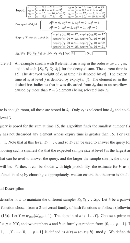
Let M=⌈logVmax⌉. The algorithm maintains(M+1)samples, denoted S0,S1, . . . ,SM. Sample Si
is said to be at “level” i. Each sample Si contains the most recent elements selected into the sample,
and when more elements enter the sample, older elements are discarded. Let ti be the most recent
timestamp of elements discarded from Si. The purpose of ti is to help in determining the range of
timestamps that are still present in the sample. The maximum number of elements in each sample Siis
α= (12/ε2)ln(8/δ).
The algorithm is described in algorithms SumInit, which describes the initialization steps for the sketch, SumProcess which describes the algorithm for updating the sketch upon receiving a new ele-ment, and SumQuery, which describes the steps for answering a query for the sum.
2.2.3 Correctness Proof
Let X denote the result returned by SumQuery(w) when a query is asked for the sum of elements within the sliding timestamp window[c−w,c]. We show that X is an(ε,δ)-estimate of V .
Algorithm 2: SumProcess(d=(v,t))
Input: v is the value of the element, and is a positive integer; t is the timestamp Task: Insert d into the sketch.
if(t<c−W)then return ; /* Discard d since it is outside the largest 1
timestamp window, and a future query will never involve d. */
Letℓ= mini|0≤i≤M,v/2ℓ<1 ; /* ℓ is an integer. */ 2
Let Pr[r=1] =v/2ℓand Pr[r=0] =1−v/2ℓ;
3
if r=1 then k←min{Z,M−ℓ+1}, where Z is the number of flips of a fair coin till the first tail;
4 if r=0 then k←0; 5 Insert(v,t)into Sℓ+k−1; 6 if|Sℓ+k−1|>αthen 7
Discard the element with the lowest timestamp in Sℓ+k−1; 8
Let t′be the timestamp of the discarded element;
9
tℓ+k−1←max{tℓ+k−1,t′}; 10
Algorithm 3: SumQuery(w)
Input: w≤W is the width of the window
Output: An estimate of the sum of all stream elements with timestamps in the range[c−w,c]
Letℓ′∈[0,M]be the smallest integer, such that for allℓ′≤ j≤M, tj<c−w;
1
if no suchℓ′exists thenℓ′←M+1;
2 ifℓ′≤M then 3 for i=ℓ′to M do ηi←∑(v,t)∈Si,t≥c−wmax(2vℓ′,1); 4 return 2ℓ′∑Mi=ℓ′ηi; 5
ifℓ′=M+1 then return ; /* Algorithm Fails */
6
Definition 2.2.1. For each element d= (v,t)∈Rw, for each level i=0,1,2, . . . ,M, random variable
xi(d)is defined as follows. Letγbe the smallest level such that v/2γ<1.
• For 0≤i<γ, xi(d) =v/2i.
• xγ(d) =1 with probability v/2γ, and xγ(d) =0 with probability 1−v/2γ.
• Forγ <i≤M, xi(d) is defined inductively. If xi−1(d) =0 then, xi(d) =0. If xi−1(d) =1, then
xi(d) =1 with probability 12 and xi(d) =0 with probability 1/2.
Definition 2.2.2. For i=0, . . . ,M, Tiis the set constructed by the following probabilistic process. Start
with Ti←φ. For each element d= (v,t)∈Rw, if xi(d)6=0, then insert(xi(d),t)into Ti.
Definition 2.2.3. For i=0, . . . ,M, define Xi=∑(u,t)∈Tiu.
Lemma 2.2.1. If d= (v,t)then E[xi(d)] =v/2i
Proof. Letγbe defined as in Definition2.2.1, i.e.γis the smallest level such that 2vγ <1. For 0≤i<γ
E[xi(d)] =v/2i, since xi(d) is a constant. For γ≤i≤M, xi(d) is a 0-1 random variable. We use
proof by induction on i to show that E[xi(d)] = Pr[xi(d) =1] =v/2i. The base case i=γ is true
since Pr[xγ(d) =1] =v/2γ by definition. Assume that for i≥γ, Pr[xi(d) =1] =v/2i. Again, using
Definition2.2.1, Pr[xi+1(d) =1] = (1/2)·Pr[xi(d) =1] =v/2i+1, thus proving the inductive step.
Lemma 2.2.2. For i=0, . . . ,M, E[Xi] =V/2i
Proof. The definitions of Xiand xi(d)yield the following.
Xi=
∑
(u,t)∈Ti
u=
∑
d=(v,t)∈Rw
xi(d)
Using linearity of expectation and Lemma2.2.1, we get:
E[Xi] =
∑
d=(v,t)∈Rw E[xi(d)] =∑
d=(v,t)∈Rw v 2i = 1 2i∑
d=(v,t)∈Rw v=V 2iLemma 2.2.3. When asked for an estimate for V , if SumQuery(w) does not fail in Step6, then it returns
2ℓ′Xℓ′ for valueℓ′selected in Step1.
Proof. Consider SumQuery(w) when asked for an estimate of the sum of elements in Rw.
Note that the level chosen by the algorithm, ℓ′, satisfies the following condition. For all levels
ℓ′≤i≤M, the most recent timestamp of the discarded elements (contained in the variable t
i in the
algorithm) is less than c−w. Thus, for all i, ℓ′≤i≤M, no element which is selected into S
iand has a
timestamp at least c−w is discarded.
Next, we argue that the contribution of each element d= (v,t)∈Rwto the value returned by the
algorithm is 2ℓ′xℓ′(d). Suppose xℓ′(d) =0. We refer to the algorithm for processing an element in SumProcess(d). The arrival of element d= (v,t)causes an insertion of(v,t)into Sifor level i< ℓ′. Note
that in computing the estimate, SumQuery(w) only uses elements from levelsℓ′or greater, element d will not contribute to the estimate returned by the algorithm.
Suppose xℓ′(d)>0. Again, referring to SumProcess(d), we note that the arrival of d causes an insertion of(v,t)into a level i≥ℓ′. In answering a query for the sum (SumQuery(w)), all elements with timestamp at least c−w which are inserted into levelsℓ′or greater are considered, and their contribution to the estimate is exactly 2ℓ′xℓ′(d). To see this, suppose v≥2ℓ′. Then, xℓ′(d) =v/2ℓ′. From Step4in SumQuery(w), the contribution of v to the estimate is 2ℓ′(v/2ℓ′) =2ℓ′xℓ′(d). Suppose v<2ℓ′. Then xℓ′(d)should be 1, since it is a 0-1 random variable. In such a case, from Step4in SumQuery(w), the contribution of d to the estimate is 2ℓ′ =2ℓ′xℓ′(d). Thus, for each d= (v,t)∈Rw, the contribution to the returned estimate is 2ℓ′xℓ′(d). The total returned estimate is exactly 2ℓ
′ Xℓ′.
Next, we will show that Xℓ′ is a good estimate for V . The following definition captures the notion of whether or not different samples yield good estimates for V .
Definition 2.2.4. For i=0, . . . ,M, random variable Xi is said to be “good” if (1−ε)V ≤Xi2i ≤
(1+ε)V , and “bad” otherwise. Define event Bi to be true if Xiis bad, and false otherwise.
Lemma 2.2.4. If|Rw| ≤α, then SumQuery(w) returns the exact answer for the sum.
Proof. Note that each element in Rwwas selected into S0when it was processed. Since theαelements
with the most recent timestamps are stored in S0, it must be true that Rw⊆S0. SumQuery will retrieve
all of Rwfrom S0and return the exact sum of Rw.
Because of the above lemma, in the rest of the proof, we assume|Rw|>α. Since each element in
the input stream is at least 1, this implies that V>α.
Definition 2.2.5. Letℓ⋆≥0 be an integer such that E[Xℓ⋆]≤α/2 and E[Xℓ⋆]>α/4. Lemma 2.2.5. Levelℓ⋆is uniquely defined and exists for every input stream R.
Proof. From Lemma 2.2.2, we have E[Xi] =V/2i. Since V >α, E[X0]>α. By the definition of
M=⌈logVmax⌉, it must be true that V ≤2Mfor any input stream R, so that E[XM]≤1. Since for every
increment in i, E[Xi] decreases by a factor of 2, there must be a unique level 0< ℓ⋆<M such that
For the next lemmas, we use a version of Hoeffding bounds from Schmidt, Siegel and Srini-vasan (70) (Section 2.1) which is restated here for convenience. Let y1,y2, . . . ,
ynbe independent 0-1 random variables with Pr[yi=1] =pi. Let Y=y1+y2+. . .+yn, and letµ=E[Y].
Lemma 2.2.6. Hoeffding’s Bound (restated from (70)): (1) If 0<δ <1, then Pr[Y >µ(1+δ)]≤e−µδ2/3.
(2) Ifδ ≥1, then Pr[Y >µ(1+δ)]≤e−µδ/3. (3) If 0<δ <1, then Pr[Y <µ(1−δ)]≤e−µδ2/2.
The next lemma helps in the proof of Lemma2.2.8. Lemma 2.2.7. If 0<a<1
2 and k≥0, then a(2
k)
≤ a
2k
Proof. It is clear by induction that 2k−1≥k. Since 0<a<1
2, we can further have a(2
k−1)
≤ak < (1/2)k. Therefore, a(2k)< a
2k.
The next lemma shows that it is highly unlikely that Bℓis true for anyℓsuch that 0≤ℓ≤ℓ⋆.
Lemma 2.2.8. For integerℓsuch that 0≤ℓ≤ℓ⋆,
Pr[Xℓ6∈(1−ε,1+ε)E[Xℓ]]< δ 2ℓ⋆−ℓ+2 Proof. Xℓ=
∑
d=(v,t)∈Rw xℓ(d)From Definition2.2.1, it follows that for some d∈Rw, xℓ(d)is a constant and for others xℓ(d)is a
0-1 random variable. Thus, Xℓis the sum of a few constants and a few random variables. Let Xℓ=c+Y
where c denotes the sum of all xℓ(d)’s that are constants, and Y is the sum of the xℓ(d)’s that are 0-1
random variables. Clearly, since the different elements of the stream are sampled using independent random bits, the random variables xℓ(d)for different d∈Rware all independent. Thus Y is the sum of
independent 0-1 random variables. LetµY =E[Y].
By linearity of expectation, we have
By the definition ofℓ⋆, E[X
ℓ⋆]>α/4. Since E[Xi] = V
2i (from Lemma2.2.2). Using Equation2.1,
we get the following inequality that will be used in further proofs.
c+µY >2ℓ ⋆−ℓ (α/4) (2.2) We first consider Pr[Xℓ>(1+ε)E[Xℓ]] Pr[Xℓ>(1+ε)E[Xℓ]] = Pr[c+Y >(1+ε)(c+µY)] = Pr[Y >µY(1+ε (c+µY) µY )] = Pr[Y >µY(1+δ′)], Whereδ′=ε(c+µY)/µY.
We consider two cases here:δ′<1 andδ′≥1.
Case I:δ′<1. Using Lemma2.2.6and the fact(c+µY)/µY ≥1, we have
Pr[Y >µY(1+δ′)] ≤ e−µYδ ′2/3 =e− ε2(c+µ Y)2 3µY ≤ e−ε2(c+µY)/3<e−ε2(2ℓ⋆−ℓ(α/4))/3 < δ 8 (2ℓ⋆−ℓ) ≤ δ/8 2ℓ⋆−ℓ
Where we have usedα= (12/ε2)ln(8/δ)andδ <1, Equation2.2and Lemma2.2.7.
Case II:δ′≥1. Using Lemma2.2.6, we have:
Pr[Y >µY(1+δ′)] ≤ e−µYδ ′/3 =e−ε(c+µY)/3 <e−2(ℓ⋆−ℓ)ln(8/δ)/ε = [(δ 8) 1/ε]2ℓ⋆−ℓ <(δ 8) (2ℓ⋆−ℓ) ≤ δ/8 2ℓ⋆−ℓ
From Case I and Case II, we have Pr[Xℓ<(1+ε)E[Xℓ]]< δ /8 2ℓ⋆−ℓ (2.3) Next we consider Pr[Xℓ<(1−ε)E[Xℓ]] Pr[Xℓ<(1−ε)E[Xℓ]] =Pr[c+Y<(1−ε)(c+µY)] =Pr[Y <µY(1−δ′)] Whereδ′=ε(c+µY)/µY
Using Lemma2.2.6and the fact(µY+c)/µY ≥1,
Pr[Y <µY(1−δ′)]≤e−µYδ ′2/2 =e− ε2(µ Y+c)2 2µY ≤e−ε2(µY+c)/2
Using Equation2.2and Lemma2.2.7,
e−ε2(µY+c)/2<[(δ 8) 3 2](2ℓ⋆−ℓ)<(δ 8) (2ℓ⋆−ℓ)≤ δ/8 2ℓ⋆−ℓ Thus, we have Pr[Xℓ<(1−ε)E[Xℓ]]< δ/8 2ℓ⋆−ℓ (2.4)
Combining Equations2.3and2.4, for 0≤ℓ≤ℓ⋆, we get
Pr[Xℓ6∈(1−ε,1+ε)E[Xℓ]] =Pr[Xℓ>(1+ε)E[Xℓ]] +Pr[Xℓ<(1−ε)E[Xℓ]]< δ /4 2ℓ⋆−ℓ Lemma 2.2.9. ℓ⋆