Dean, Nema, and Nugent, Rebecca (2013)
Clustering student skill set
profiles in a unit hypercube using mixtures of multivariate betas.
Advances
in Data Analysis and Classification, 7 (3). pp. 339-357. ISSN 1862-5347
Copyright © 2013 Springer-Verlag Berlin Heidelberg
A copy can be downloaded for personal non-commercial research or
study, without prior permission or charge
Content must not be changed in any way or reproduced in any
format or medium without the formal permission of the copyright
holder(s)
When referring to this work, full bibliographic details must be given
http://eprints.gla.ac.uk/85168/
Deposited on: 1 July 2014
Enlighten – Research publications by members of the University of Glasgow http://eprints.gla.ac.uk
Clustering Student Skill Set Profiles in a Unit
Hypercube using Mixtures of Multivariate Betas
Nema Dean
∗1and Rebecca Nugent
21School of Mathematics & Statistics, University of Glasgow
2Department of Statistics, Carnegie Mellon University
31 July 2013
Abstract
This paper presents a finite mixture of multivariate betas as a new model-based clustering method tailored to applications where the feature space is constrained to the unit hypercube. The mixture component densities are taken to be conditionally independent, univariate unimodal beta densities (from the subclass of reparameter-ized beta densities given by Bagnato and Punzo, 2013). The EM algorithm used to fit this mixture is discussed in detail, and results from both this beta mixture model and the more standard Gaussian model-based clustering are presented for simulated skill mastery data from a common cognitive diagnosis model and for real data from the Assistment System online mathematics tutor (Feng et al, 2009). The multivariate beta mixture appears to outperform the standard Gaussian model-based clustering approach, as would be expected on the constrained space. Fewer components are selected (by BIC-ICL) in the beta mixture than in the Gaussian mixture, and the resulting clusters seem more reasonable and interpretable. This article is in technical report form, the final publication is available at
http://www.springerlink.com/openurl.asp?genre=article&id=doi:10.1007/s11634-013-0149-z.
Keywords:Mixture Model Clustering, Multivariate Beta Densities, Skill Set Profiles, Unit Hypercube
1
Introduction
One of the primary goals in educational research is to accurately estimate the extent of students’ mastery of different skills. While assessment of students’ current knowledge is obviously crucial in education, this estimation also has applications when teachers are interested in grouping similar students based on their skill mastery. For example, students showing consistent high levels of aptitude may be selected for an advanced class or, in cases where teaching assistants are available, students with similar deficiencies could more efficiently receive extra instruction as a group.
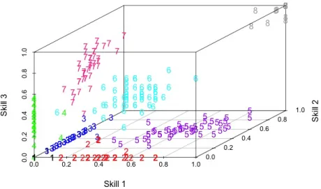
Cognitive diagnosis models (CDMs) are commonly used in estimating skill mastery based on students’ correctness of response to items involving the skills of interest. A review and comparison of various different CDMs can be found in DiBello et al (2007) and Rupp et al (2010). For each student, we estimate a set of individual skill masteries, or a skill set mastery profile. Skill mastery is typically estimated on the [0,1] range, with 0 indicating total lack of mastery and 1, perfect mastery. The skill set profile (and its estimate) for K skills then lies in the K-dimensional unit hypercube, [0,1]K. Figure 1
shows the three-dimensional unit hypercube feature space for the skill set profile estimates for 400 students simulated from a common CDM, theDeterministicInputs,Noisy “And” gate (DINA) model (Junker and Sijtsma (2001), Torre (2009), further details in Section 3.2.1). The students’ original skill set profiles are shown by character type; for example, the group in the upper right corner corresponds to students with perfect mastery for all three skills. Recovery of these original profile groups is our goal.
Figure 1: 3-D skill set profile estimates for 400 simulated students
Estimating these skill set profiles using even basic CDMs can be extremely com-putationally intensive, involving Markov Chain Monte Carlo estimates that themselves can only reasonably be found for a limited number of students and skills. Ayers et al (2008, 2009) introduced a simple skill profile estimate (further details given in Section 3.2.2) which, in combination with cluster analysis methods, performed as well at recov-ering students’ skill mastery profiles. However, the clustrecov-ering methods used in that work (e.g. K-Means, hierarchical agglomerative clustering, model-based clustering) did not accurately reflect the restricted hypercube feature space commonly found in educational research.
This paper focuses on extending the common mixture based clustering approach for use with the flexible (multivariate) beta distribution. It assumes each mixture component can be modeled by a product of conditionally independent, univariate beta densities (one for each dimension, here skill). Introduced in Section 2.1, this model is naturally tailored
due to Bagnato and Punzo (2013) as well as the EM algorithm for fitting the mixture. We compare this approach to the standard Gaussian mixture model for continuous (and transformed) data. We provide simulation results from the popular DINA model (Section 3.2.1) and results on data from an online classroom tutoring system (Assistments, Feng et al (2009), Section 3.3). Finally, the paper concludes with discussion and caveats for the two approaches; computational considerations and possible future extensions follow in Section 4.
2
Mixture Model Clustering
Broadly, cluster analysis is a set of methodologies for grouping similar observations to-gether in classes or clusters. These clusters are chosen such that the observations in each cluster are more similar to each other than to observations in other clusters and are assumed to estimate true, unknown underlying groups. Model-based clustering is a particular approach based on finite mixture models (McLachlan and Peel, 2000), that has become increasingly popular across diverse applications due to the flexibility of its estimated cluster shapes and sizes, its automatic selection of the number of clusters, and software and advanced extensions availability (Fraley and Raftery, 1998, 2002; Fraley and Raftey, 2007; Raftery and Dean, 2006; McLachlan and Peel, 1999). We adopt this model-based approach here.
We assume that the data X = {x1, . . . ,xK} are an independently and identically
distributed sample from some unknown population density f(x) where each group g in the population is represented by a mixture component fg(x). The population density
f(x) is then a weighted mixture of these components:
f(x) = G X g=1 πg·fg(x;θg) where 0≤ πg ≤ 1, P
πg = 1. The parameters for a mixture model with a given number
of components can be easily estimated using the EM algorithm (Dempster et al, 1977). The E-step estimates missing data identifying the probabilities of component membership for each observation, given the current parameter estimates; the M-step calculates the maximum likelihood estimates of the model parameters, given the current estimates of component membership. The two steps are alternated until convergence. The Bayesian Information Criterion (Schwarz, 1978) is used (as an approximation for Bayes factors) to choose G, the number of components, that best fits the data (see Section 2.1.4). Each fitted mixture component is then usually identified as a cluster; observations are assigned to the component/cluster with highest posterior probability of membership. Comprehensive reviews of the methodology can be found in McLachlan and Peel (2000) and Fraley and Raftery (2002).
Commonly, fg is assumed to be Gaussian (i.e. θg = {µg,Σg}). In particular, the
M-step for Gaussian component densities has closed form solutions for the maximum likelihood parameter estimates (see Fraley and Raftery, 2002). If this assumption is violated, it is possible that the number of components (and so the number of popula-tion groups) will be overestimated, as subgroups of Gaussian mixture components are needed to estimate an underlying non-Gaussian group (Lindsay, 1995; McLachlan and Peel, 2000). Work done by Baudry et al (2010) and Hennig (2010a,b) and Dean and Nu-gent (2013) have explored ways of identifying how/when to merge mixture components
to create clusters under these circumstances. This paper will not look at this particular extension of model-based clustering but instead focus on assuming a more appropriate underlying distribution.
2.1
Finite Mixture of Beta Distributions
Since each profile ofKskill mastery estimates will lie in theKdimensional unit hypercube
[0,1]K, it seems desirable to use a component distribution that is defined only on the unit hypercube (unlike the multivariate Gaussian defined on the whole real spaceRK, although
we will show it can work quite well in some circumstances). The (standard) beta density given by
f(x|α, β) = 1
B(α, β)x
α−1
(1−x)β−1, α, β >0 (1)
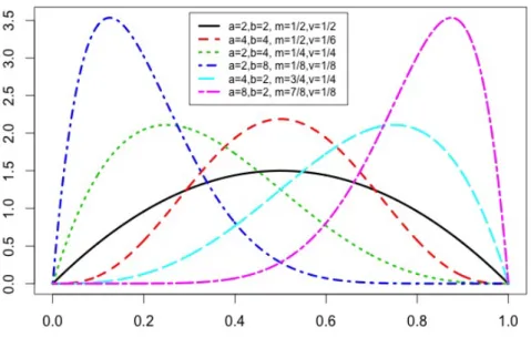
where B(α, β) = Γ(Γ(αα)Γ(+ββ)). The density is defined on x ∈ [0,1], and, as such, seems well suited as a univariate component density for this application. The beta density is also extremely flexible (depending on the values of its parameters). Figure 2 gives some examples of the density shapes available for this parametric family. The beta density with α= 5, β = 2might correspond to a group of students with moderate to high mastery of a skill; the density with α = 1, β = 3 might be a group of students who tend to struggle with that same skill.
Figure 2: Beta densities with different parameter values; α values given by a, β values by b.
2.1.1 Properties of the Beta Density
The beta density is symmetric when the shape parameters,αandβ, are equal and skewed otherwise. Its mean is given by α+αβ and variance by (α+β)2αβ(α+β+1). However, there are
two properties of this distribution that make it problematic in the model-based clustering context:
• it is bimodal for α <1and β <1;
• there is no closed form maximum likelihood estimation solution for α, β.
The first property means that if we allow solutions for shape parameter estimation where
both α, β < 1, we will have a component density with two modes, one towards 0 and
another towards 1. This bimodality makes the interpretation of the component as a one-group cluster problematic (unimodal component densities are desired). Dean and Nugent (2011) looked at constraints on the optimisation as a solution for bimodality in mixtures of beta densities; this paper will take a different, more stable approach.
In particular, we adopt an alternative method of specifying the beta distribution that allows only unimodal univariate densities, first explored by Bagnato and Punzo (2013) focusing on restricted unimodal reparameterizations of the gamma and beta densities. This subclass of beta densities is given by:
f(x|m, v) = x
m/v(1−x)(1−m)/v
B mv + 1,1−vm + 1 (2)
where m ∈[0,1], v > 0, and v = α+1β−2. As with the standard beta density, there is no closed form solution for the maximum likelihood estimates of m and v. EM algorithm starting values can be found using the method of moments.
According to Bagnato and Punzo (2013), the two parameterizations in Equations (1), (2) are equivalent for α, β > 1. This subclass excludes beta densities that are bimodal, unlimited (reverse) J-shaped, or uniform. Note that the remaining betas still have a large degree of flexibility (Figure 3).
Since the usual EM algorithm for estimating component parameters requires max-imum likelihood estimates, the second undesirable property seems to preclude us from fitting mixtures of beta distributions. We discuss our proposed solution in Sections 2.1.2, 2.1.3.
2.1.2 Mixtures of Multivariate Beta Distributions
Mixtures of univariate beta distributions have been previously looked at by Ji et al (2005) in the context of modelling correlations between gene-expression levels, particularly to systematically identify “large” correlations. In our setting, mixtures of univariate beta distributions would refer to looking for clusters of students based on their mastery es-timates for only one skill (or an overall mastery). We are more interested in a general K-skill framework and, as such, need to fit mixtures of multivariate betas.
To model multivariate data in the unit hypercube, we use the local independence (or conditional independence) assumption common to latent class analysis (Lazarsfeld and Henry, 1968). This assumption allows independence between variables conditional on the component membership. It is less restrictive than an unconditional independence assumption but still fairly strong.
Figure 3: Densities for unimodal betas with different parameter values; α values given by a, β values by b; corresponding m and v parameters also given.
Given this assumption and the Bagnato and Punzo (2013) beta density reparameter-ization, forK-dimensional multivariate dataxi = (xi1, . . . , xiK), the multivariate density
for the gth component is given by
fg(xi|mg,vg) = K Y k=1 fgk(xik|mgk, vgk) (3) where fgk(xik|mgk, vgk) = xmgk/vgk ik (1−xik) (1−mgk)/vgk B(mgk vgk + 1, 1−mgk vgk + 1) . Then the finite mixture of Gmultivariate beta distributions is given by
f(xi) =
G X
g=1
πgfg(xi|mg,vg). (4)
2.1.3 Fitting the Mixture of Multivariate Beta Densities
We use the expectation-maximization (EM) algorithm (Dempster et al, 1977) to estimate the model parameters. As usual for the mixture model context, we introduce missing data zi to identify the component membership of each observation xi, defined as follows:
The algorithm proceeds as follows:
1. Initialize the zig either by assigning the data using quantiles to each ofGgroups in
the univariate setting (i.e. split the data into G quantiles; observations, xi, whose
value falls in the kth quantile havez
ik set to 1 and zij set to 0 ∀j 6=k) or assigning
the data using k-means (or some other multivariate assignment) in the multivariate case (i.e. k-means is run on the data for k=G; if k-means assigns observation xi to
cluster k then we set zik to be 1 and zij set to 0 ∀j 6=k).
2. M-Step: Given the current values for theˆzi’s, estimate the set of parameters
(π1, . . . , πG,m1,v1, . . . ,mG,vG) by:
(a) ˆπg =
Pn i=1zˆig
n
(b) Obtain a numerical maximizer for mgk, vgk by solving n
X
i=1
ziglog(fgk(xik|mgk, vgk))1[xik6=NA]
subject tomgk ∈[0,1]and vgk >0 fork = 1, . . . , K and g = 1, . . . , G,
where1[ ] is the indicator function (here used to check non-missingness) equal
to 1 if the statement in [ ] is true and 0 otherwise. Starting values for the mgk, vgk in the numerical optimiser are taken to be the previous M-step
esti-mates or method of moments estiesti-mates in the initial M-step.
3. E-Step: Given the current parameter estimates from the M-step, compute
ˆ zil = ˆ πlfl∗(xi|mˆl,vˆl) PG g=1πˆgfg∗(xi|mˆg,vˆg) for i= 1, . . . , n;l = 1, . . . , G where fg∗(xi|mˆg,vˆg) =QKk=1fgk(xik|mˆgk,vˆgk)c(xik)
and c(xik) = 1 if xik 6=N A and 0 otherwise.
4. Repeat the M-step and E-step until convergence is reached.
Note that the conditional independence assumption means that, in the event of missing data for some variables on some observations, the incomplete observations can still be used in the estimation of the parameters for which data are observed and the observation component/cluster membership can still be estimated.
The estimated zˆils will typically fall anywhere on the range of the interval [0,1]. To
get hard classifications for points to components, we can define the hard label estimate,
˜
zi as:
˜
zil = 1 if arg max
g zˆig =l, and0 otherwise.
2.1.4 Selecting the Number of Mixture Components
The usual method for selecting the number of mixture components G is to fit mixtures with different numbers of components, scoring each proposed model using some infor-mation criterion. The model with the optimal criterion value and consequently the best number of components is selected.
In Gaussian component mixtures, the most common information criterion used is the Bayesian Information Criterion (BIC), first introduced by Schwarz (1978) and further dis-cussed in Kass and Raftery (1995), which we define for the G component, K-dimensional beta mixture model MG as:
BIC(MG) = 2×maximized log likelihood of modelMG−ν×log(n)
where G is the number of components, ν is the number of independent parameters (= (2×G×K) +G−1), and n is the number of observations in the data. The model with the largest BIC is considered the best fit for the data; its corresponding number of components is chosen for G.
Ji et al (2005) found that BIC did not perform well in selecting the number of com-ponents in univariate beta mixture simulations and suggested the BIC-ICL criterion as a preferred alternative. The BIC-ICL criterion is defined as follows:
BIC-ICL(MG) = BIC(MG)−2×EN(ˆz)
where EN(ˆz) = −Pni=1PGg=1zˆiglog(ˆzig) is the estimated entropy of the fuzzy
classifi-cation given by the final E-step value of zˆ for model MG. Again, the model with the
highest BIC-ICL and its corresponding number of components are chosen as the best fit to the data. The range of number of components being fit was allowed to increase until the BIC(-ICL) values began to decrease.
2.1.5 Competing model strategies
In situations where the data are continuous on a restricted space, standard (Gaussian mixture) model-based clustering is often applied, ignoring the possible violation of model assumptions. Although this model is not tailored to the unit hypercube space, it can still be a useful tool.
Another common approach is to transform or normalise the data prior to applying standard mixture models. For xi ∈[0,1], the most commonly used transformation is the
arcsine transformation (Sokal and Rohlf, 1981), mapping the[0,1]domain to the[0, π/2]
range by taking the square root of the observation and then finding the arc sine value in radians, i.e.
yik =f(xik) = sin−1( √
xik).
In this paper we apply Gaussian model-based clustering to the resulting transformed data and report the results. The cluster means and variances estimated on the trans-formed data can be easily transtrans-formed back onto the original scale by using the inverse transformation, i.e.
˜
µg =f−1(µg) = (sin(µg))2.
3
Results
The Gaussian component model-based clustering was implemented using the mclust
library (Fraley et al, 2012) in the R programming language (R Core Team, 2012). R code to fit the EM algorithm for the beta mixture is available at
3.1
Assessing Performance
The Adjusted Rand Index, ARI, (Hubert and Arabie, 1985) is a measure used to compare two different clustering partitions on the same data. It counts the proportion of observa-tion pairs where the clusterings agree (i.e. both partiobserva-tions put the pair of observaobserva-tions in the same cluster or both put them in different clusters) and adjusts for random chance matching. The expected value of the ARI is zero under random assignment; an ARI of 1 indicates the two clusterings (or the clustering and the true set of class labels) are identical. For our results, we report both the misclassification rate and the corresponding ARI value.
3.2
Simulation with Known Group Structure
In order to assess the ability to recover known group structure, we simulate from the DINA model, a common CDM (detailed in Section 3.2.1). The simulated values can then be used to estimate skill set profiles which fall in groups on the unit hypercube. In practice, CDM estimation of the skill set profiles often requires lengthy MCMC-type procedures which are impractical or computationally infeasible for scenarios with large numbers of questions or skills. We then use the resulting estimated skill set profiles to identify the different profile groups present in a population. In this paper, we instead calculate quicker estimates of the students’ skill mastery profiles (detailed in Section 3.2.2) and then apply our finite mixture of betas to cluster the students. However, note that the finite mixture of betas is applicable to any estimates that lie in the unit hypercube (including those obtained through MCMC).
3.2.1 Simulation from the DINA Model
Each student has a true skill-set profile γi = (γi1, γi2, . . . , γiK) whereγik is 1 if student i
has mastered skill k and 0 otherwise. Estimation of the skill set profiles is done using a N×J student response matrix Y whereYij is 1 if studentianswered item j correctly, 0
if answered incorrectly and NA if studenti did not see itemj and a J×K skill transfer
Q-matrix (Barnes, 2005) where qjk is 1 if item j required skill k, 0 otherwise. Here N
is the total number of students, J is the total number of questions being examined, and K is the total number of skills. Under the DINA model (Junker and Sijtsma, 2001), the probability of a correct response given ηij (a function of γi) is
P(Yij|ηij, sj, gj) = (1−sj)ηijg 1−ηij j (5) whereηij = QK k=1γ qjk
ik (= 1 if studenti has all the skills required for itemj, 0 otherwise),
representing the conjunctive assumption that essentially all required skills should be mastered for the student to answer an item correctly; and sj = P(Yj = 0|ηij = 1)
and gj = P(Yij = 1|ηij = 0) are slip and guess parameters (here randomly drawn from
Uniform[0, 0.01] for illustrative purposes).
Returning to the Figure 1 scenario, we simulate responses from the DINA model for N =400 students given their true skill set profiles forK =3 skills (23 = 8possible profiles
= the true number of groups) usingJ =30 items (18 = 6×3single skill questions for each skill, 9 = 3×3 double skill questions for each possible pair of skills and three questions involving all three skills). The rows of Q are either (1,0,0), (0,1,0) or (0,0,1) for single skill questions, (1,1,0), (0,1,1) or (1,0,1) for double skill questions or (1,1,1) for triple skill questions. Students were randomly assigned 15 questions.
3.2.2 Skill Mastery Estimates
Rather than use lengthy MCMC estimation procedures to findγˆi, previous papers (Ayers et al, 2008, 2009) have discussed the use of quicker skill mastery estimates from the response data and skill transfer matrix in conjunction with clustering methods to estimate the original profile group. In this paper, we use the capability estimate described in Ayers et al (2008) and below in equation (6). This student-skill estimate matrix, B, is defined as: Bik = PJ j=11[Yij6=N A]·Yij ·qjk PJ j=11[Yij6=N A]·qjk i= 1, . . . , N;k= 1, . . . , K (6)
where 1[ ] is the indicator function equal to 1 if the statement inside the brackets is true
and 0 otherwise. Our unknown skill set masteries, γik, are estimated by the Bik. Note
that although the trueγi’s will fall only on the hypercube corners, the Bik estimates can
lie anywhere within the hypercube. After fitting the beta mixture model, the clusters can be mapped to the closest corners, or the cluster centres could be used as estimates if it is believed that skill mastery lies on a spectrum rather than a binary scale.
3.2.3 Simulation Results
We estimate the three-skill set profiles, with all 8 (possible) groups, for our 400 simulated students (see Figure 4). Note that some points in the hypercube represent more than one observation (e.g. 46 students were estimated to have the point (1,1,1)). The questions requiring multiple skills are responsible for the migration of skill set profile estimates towards the bottom-left (0,0,0) corner, since not mastering just one of several required skills corresponds to a reduction in the mastery estimates for all the required skills for that item.
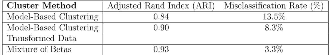
A summary of our results is given in Table 1. Model-based clustering with Gaussian components selects 14 “EEV” (equal volume and shape but variable orientation) compo-nents which gives a misclassification rate of 13.5% and an ARI of 0.84 when compared to the true profile groups. Model-based clustering with Gaussian components applied to the arcsine transformed data also selects 14 “EEV” components, but the misclassification is improved to 8.25% with an ARI of 0.90. This improvement is due to better estimation of the main groups, with the extra components being small groups (e.g. singletons).
The finite mixture of multivariate betas will not fit beyond eight components (likely due to difficulty in finding sensible starting values for number of components higher than the truth), and BIC-ICL selectsG= 8 as the best fit, the correct number of groups. The misclassification rate drops to 3.25%, and the ARI increases to 0.93.
Table 1: Summary of Adjusted Rand Index and misclassification rates for simulated data Cluster Method Adjusted Rand Index (ARI) Misclassification Rate (%)
Model-Based Clustering 0.84 13.5%
Model-Based Clustering 0.90 8.3%
Transformed Data
Mixture of Betas 0.93 3.3%
Figure 4 shows the misclassifications (compared to the underlying true groups, lighter coloured stars) for both the beta and Gaussian mixture approaches. For the beta mixture,
Figure 4: Comparing the beta and Gaussian mixture results; misclassified obs. given by stars
the misclassifications are from singletons or pairs of points lying close to the boundary of two groups. The Gaussian mixture suffers from these types of misclassifications as well but also from true groups being split into more than one component.
In general, any set of appropriate skill mastery estimates that lie in (or could be mapped into) the unit hypercube can be clustered with this approach. For example, a scaled version of sum scores (Henson et al, 2007) could be used in place of the capability estimates. Similarly, the DINA model is just one common CDM estimating skill mastery; similar analyses could be done with other CDMs like the NIDA or RedRUM (for example, see Rupp et al, 2010).
3.3
Assistment System: Online Tutoring Data
We examine a subset of 26 items requiring three skills from the Assistment System online mathematics tutor (Feng et al, 2009). We have student response data from 551 stu-dents on the skills Evaluating Functions, Multiplication, and Unit Conversion. Unlike our previous simulation, the Q-matrix is unbalanced; Evaluating Functions appears in eight items, Multiplication in 20 items, and Unit Conversion in two items. Note that Unit Conversion only occurs in conjunction with the other two skills. This imbalance means that estimation will be more difficult due to the conjunctive assumption. Our skill estimates, e.g. Equation (6), will be pulled away from the corners of the hypercube as any multiple skill question answered incorrectly will penalize all corresponding skill estimates even if only a subset of unmastered skills led to the error.
3.3.1 Summary of Student Responses
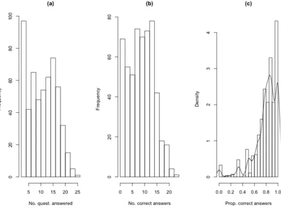
Students were shown a random selection from the 26 questions, and, for the purposes of this analysis, we assume that the students answered all shown questions. That is, missing values are assumed to be due to the student not seeing the question rather than refusing to answer. The students attempted different numbers of questions (see
Figure 5(a)). The lower and upper quartiles for the number of questions answered are six and sixteen; all answered at least two. The lower and upper quantiles for the number of questions answeredcorrectly are five and thirteen with corresponding histogram in Figure 5(b). Finally, ignoring which skills belong to which question, we look at the proportion of attempted questions correctly answered by each student (a rough approximation of overall mastery). Gratifyingly, the lower and upper quartiles for this proportion are 0.75 and 0.93. We add a kernel density estimate to the corresponding histogram in Figure 5(c) as a possible preview of the number of different mastery groups.
Figure 5: Histograms of (a) number of questions answered by students, (b) number of questions answered correctly by students and (c) proportion of correct answers
3.3.2 Clustering Student Overall Ability
It might first be of interest to group students according to overall ability (i.e. proportion of total attempted questions correctly answered). If we ignore the restricted sample space ([0,1]) and apply standard model-based clustering with Gaussian components to this uni-variate summary data, we still struggle with the problem of replicated observations (here this occurs numerous times; for example, 9 students observed at the value 0, 13 observed at 0.33, 25 observed at 0.8, etc). These points likely will be modeled as Gaussian compo-nents with zero variance, corresponding to an infinite likelihood. In general, we will be unable to fit models assuming clusters with unequal variance, but forcing equal variances across clusters still can give an overly large number of components (as selected by BIC). For example, when clustering the overall ability estimates from Figure 5(c), the BIC for Gaussian model-based clustering is maximized at 11 components. The corresponding mixture density estimate (and component density estimates weighted by corresponding
the density is overly “wiggly” due to the extra components associated with the duplicated observations; furthermore, components overfitting to small numbers of observations are less useful for broad summarization or classification.
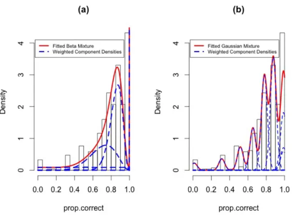
Next we fit mixtures of betas to the student’s overall proportion of questions correctly answered. BIC-ICL decisively selects four components as being the best fit (1710.14 vs 1607.14). The final parameter estimates are given in Table 2; the estimated density is overlaid as a solid line (with weighted component densities as dashed lines) on the histogram of proportion of correct answers in Figure 6 (a).
Figure 6: (a) Density estimate for the four component fitted beta mixture (solid line) and (b) the eleven equal variance components fitted Gaussian mixture (solid line). Individual components in the mixtures (weighted by the mixing proportions) are given by dashed lines.
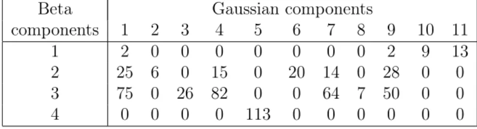
The first beta component appears to be a close-to-uniform noise component (centred at 0.5 with fairly large variance) soaking up lower-valued observations not assigned to other components. The fourth component has only students answering all questions correctly. Note that 20.5% of the students got a proportion correct value of exactly 1, hence the extreme peakedness of this component capturing these students (this component’s dashed line is obscured by the mixture line in Figure 6 (a)). As expected, this mixture seems to give a smoother density estimate than the Gaussian model-based clustering estimate. The cross-classification table for the Gaussian components (columns) and beta components (rows) is in Table 3.
Table 2: Mixing proportions, means, and variances for the four beta mixture components Component 1 2 3 4 ˆ πg 0.09 0.27 0.44 0.21 Mean 0.50 0.70 0.85 1.00 Variance 0.083 0.018 0.005 1e−7
Table 3: Cross-classification Table: Gaussian vs beta component assignments
Beta Gaussian components
components 1 2 3 4 5 6 7 8 9 10 11
1 2 0 0 0 0 0 0 0 2 9 13
2 25 6 0 15 0 20 14 0 28 0 0
3 75 0 26 82 0 0 64 7 50 0 0
4 0 0 0 0 113 0 0 0 0 0 0
3.3.3 Multivariate Clustering of Student Skill Estimates
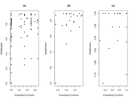
In Figure 7, we show the three-dimensional skill mastery capability estimates (see Equa-tion (6)) for our subset of Assistment data. As there were only two quesEqua-tions involving the Unit Conversion skill, there are only three possible values for its skill mastery estimate: 0, 0.5, and 1. There are 101 students with an estimated mastery of zero, 23 students with 0.5, and 35 students with one (perfect mastery). We condition on these three planes and separately cluster each of the three 2-D conditional planes of skill mastery for Evaluating Functions and Multiplication. Conditioning was shown in Nugent et al (2009) to be a more sensible approach for this data rather than direct three-dimensional multivariate clustering (as the extreme coarseness of the distribution of Unit Conversion overwhelms more interesting clustering information within the 2-D subplanes). The corresponding conditional planes are shown in Figure 8.
Model-based clustering with Gaussian components chooses seven “VEI” (varying vol-ume, equal shape diagonal) components for the first (0) plane, two “EEV” (equal volume and shape and varying orientation) components in the second (0.5) plane and seven “EEV” components in the third (1) plane (shown in Figure 9). As before, the use of Gaussian densities tends to give a larger number of components resulting in a larger variability in the density estimate. In Figure 9, we see that the resulting clusters within the sub-planes seem to be defined by variation for both Evaluating Functions and Multiplication.
Using a mixture of beta component densities, BIC-ICL selects three components in the first Unit Conversion plane (0), one component in the second plane (0.5) and two components in the third plane (1). Unlike our previous results, the clusters now tend to be driven by the Evaluating Function values (see Figure 10). The clusters in the first plane are students with zero mastery in both skills (diamond in Figure 10(a)), students with non-zero mastery in both skills (circles in Figure 10(a)) and students with zero mas-tery in Evaluating Functions and non-zero masmas-tery in Multiplication (triangles in Figure 10(a)). The clusters in the third plane are students with perfect (1) mastery in Evaluating Functions (triangles in Figure 10(c)) and non-perfect mastery in Evaluating Functions
Figure 7: 3-D skill mastery estimate scatterplot for the Assistment data
Figure 8: Skill mastery estimates for Evaluating Function & Multiplication in the (a) zero, (b) 0.5, and (c) 1 Unit Conversion planes
Figure 9: Skill mastery estimates for Evaluating Function & Multiplication in the (a) zero, (b) 0.5, and (c) 1 Unit Conversion planes; Gaussian component assignments given by symbol
Figure 10: Skill mastery estimates for Evaluating Function & Multiplication in the (a) zero, (b) 0.5, and (c) 1 Unit Conversion planes; beta component assignments given by symbol
interpretable from an educational testing point of view.
4
Discussion
In general, both Gaussian component and beta component mixture models can give use-ful clustering results. In an effort to best fit the underlying population density, the use of Gaussian components tends to select a larger number of components with a correspond-ingly more variable density estimate. However, its use also assumes an unconstrained fea-ture space. Modeling beta components tends to give a more useful summarization when smaller numbers of components are desired or when the feature space is constrained (in our application, by the unit hypercube). In our simulations, we also saw that the correct number of components was selected for skill set profile data generated from the DINA model (while the number of Gaussian components overestimated the correct number of true profile groups).
The examples given in this paper were chosen to be three-dimensional for ease of illustration and discussion of results. Mixture models using Gaussian components or beta components are more generally applicable to higher dimensions, and their greatest usefulness is in such higher-dimensional problems where the estimation of standard CDMs is not feasible.
Computational issues can arise with fitting beta mixtures due to rounding error (par-ticularly when taking the product of a large number of probability densities in the E-step of the EM algorithm). Suitable care must be taken to avoid this problem as much as possible. Other potential problems with multivariate data are associated with the specifi-cation of EM starting parameter values. In this paper, K-Means clustering was used as a quick and reasonable choice to give reasonable starting estimates for the zmatrix in the E-step. However, these estimates may not always be useful and, like all approaches, the fitting of the mixture of beta densities may be plagued by entrapment in local maxima. In addition to possibly using several sets of K-Means starting values, multiple random start approaches could be used to try to avoid the issue of local optima. Numerical optimisa-tion in the mixture of the subclass of beta densities must also be carefully constrained to the correct parameter space and issues with precision (due to the calculation of the log beta function in the log-likelihood) may occasionally arise.
One restriction with the proposed beta mixture approach is the assumption of con-ditional independence between variables within the components. This assumption is not necessarily required when using Gaussian components in model-based clustering. An alternative model could be to specify more general unimodal multivariate densities de-fined on the unit hypercube that allow dependence. In practice thus far, however, this assumption does not appear overly stringent.
The beta mixture model approach in this paper was applied to skill mastery estimates as given by equation (6) but is more widely applicable to any estimates from CDMs that fall in the unit hypercube. One clear problem with the estimates as given by equation (6) is the lack of uncertainty associated with the estimate. For example, we would be much less confident in a value of one estimated from only one question involving a particular skill than a value of one estimated from ten questions. An alternative approach would be to look at the number of questions involving the skill and the number of correct answers (e.g., the sum scores approach of Henson et al, 2007) and model these directly using a mixture of binomial densities instead of beta densities. This approach would have the
disadvantage that it could not be applied to most CDM estimates that lie directly in the unit hypercube.
This mixture of multivariate betas could also be applied to multivariate data with variables made up of correlations, for example time-wise correlation in gene-expression levels, or for modelling recovery rates of loans of different types. Regardless of application, though, one large advantage of working within the mixture model framework means that variable selection techniques developed by Raftery and Dean (2006) and extended by Maugis et al (2009) could be adapted to the mixture of betas setting. Similarly, extensions to mixture of experts or mixed membership models could be developed.
References
Ayers E, Nugent R, Dean N (2008) Skill set profile clustering based on student capability vectors computed from online tutoring data. In: Baker R, Barnes T, Beck JE (eds) Proceedings of the 1st International Conference on Educational Data Mining, Montreal, Canada, pp 210–217
Ayers E, Nugent R, Dean N (2009) A comparison of student skill knowledge estimates. In: Barnes T, Desmarais M, Romero C, Ventura S (eds) Proceedings of the 2nd Inter-national Conference on Educational Data Mining, Cordoba, Spain, pp 1–10
Bagnato L, Punzo A (2013) Finite mixtures of unimodal beta and gamma densities and
the k-bumps algorithm. Computational Statistics 28(4), doi 10.1007/s00180-012-367-4
Barnes TM (2005) The Q-matrix method: Mining student response data for knowledge. In: Beck JE (ed) Educational Data Mining: Papers from the 2005 AAAI Workshop, American Association for Artificial Intelligence, Menlo Park, California, Technical Re-port WS-05-02, pp 39–46
Baudry JP, Raftery AE, Celeux G, Lo K, Gottardo R (2010) Combining mixture compo-nents for clustering. Journal of Computational and Graphical Statistics 19(2):332–353 Dean N, Nugent R (2011) Comparing different clustering models on the unit hypercube. In: Proceedings of the 58th World Statistics Congress, International Statistical Insti-tute, Dublin, Ireland
Dean N, Nugent R (2013) Mixture model component trees: Visualizing the hierarchical structure of complex groups. Tech. rep., University of Glasgow, in preparation
Dempster AP, Laird NM, Rubin DB (1977) Maximum likelihood from incomplete data via the EM algorithm. Journal of the Royal Statistical Society, Series B: Methodological 39(1):1–38, with discussion
DiBello L, Roussos L, Stout W (2007) Review of cognitively diagnostic assessment and a summary of psychometric models. In: Rao CR, Sinharay S (eds) Handbook of Statistics, 26, Elsevier, Amsterdam, pp 979–1030
Feng M, Heffernan N, Koedinger K (2009) Addressing the assessment challenge in an intelligent tutoring system that tutors as it assesses. The Journal of User Modeling and User-Adapted Interaction 19(3):243–266
Fraley C, Raftery AE (1998) How many clusters? which clustering method? - answers via model-based cluster analysis. Computer Journal 41:578–588
Fraley C, Raftery AE (2002) Model-based clustering, discriminant analysis, and density estimation. Journal of the American Statistical Association 97(458):611–612
Fraley C, Raftey AE (2007) MCLUST version 3 for R: Normal mixture modeling and model-based clustering. Tech. Rep. 504, Department of Statistics, University of Wash-ington
Fraley C, Raftey AE, Murphy TB, Scrucca L (2012) mclust version 4 for R: Normal mixture modeling for model-based clustering, classification, and density estimation. Tech. Rep. 597, Department of Statistics, University of Washington
Hennig C (2010a) Methods for merging Gaussian mixture components. Advances in Data Analysis and Classification 4(1):3–34
Hennig C (2010b) Ridgeline plot and clusterwise stability as tools for merging Gaussian mixture components. In: Locarek-Junge H, Weihs C (eds) Classification as a Tool for Research, Springer, Berlin, pp 109–116
Henson J, Templin R, Douglas J (2007) Using efficient model based sum-scores for con-ducting skill diagnoses. Journal of Education Measurement 44(4):361–376
Hubert L, Arabie P (1985) Comparing partitions. Journal of Classification 2(1):193–218 Ji Y, Wu C, Liu P, Wang J, Coombes KR (2005) Applications of beta-mixture models in
bioinformatics. Bioinformatics 21(9):2118–2122
Junker BW, Sijtsma K (2001) Cognitive assessment models with few assumptions and connections with nonparametric item response theory. Applied Psych Measurement 25(3):258–272
Kass RE, Raftery AE (1995) Bayes factors. Journal of the American Statistical Associa-tion 90(430):773–795
Lazarsfeld PF, Henry PW (1968) Latent Structure Analysis. Houghton Mifflin, Boston Lindsay BG (1995) Mixture Models: Theory, Geometry, and Applications. NSF-CBMS
Regional Conference Series in Probability and Statistics, Vol. 5, Institute of Mathe-matical Statistics, Hayward
Maugis C, Celeux G, Martin-Magniette ML (2009) Variable selection in model-based clus-tering: A general variable role modeling. Computational Statistics and Data Analysis 53(11):3872–3882
McLachlan G, Peel D (1999) The EMMIX algorithm for the fitting of normal and t-components. Journal of Statistical Software 4(2):1–14
Nugent R, Ayers E, Dean N (2009) Conditional subspace clustering of skill mastery: Iden-tifying skills that separate students. In: Barnes T, Desmarais M, Romero C, Ventura S (eds) Proceedings of the 2nd International Conference on Educational Data Mining, Cordoba, Spain, pp 101–110
R Core Team (2012) R: A Language and Environment for Statistical Computing. R Foundation for Statistical Computing, Vienna, Austria, URLhttp://www.R-project. org/, ISBN 3-900051-07-0
Raftery AE, Dean N (2006) Variable selection for model-based clustering. Journal of the American Statistical Association 101(473):168–178
Rupp AA, Templin J, Henson RA (2010) Diagnostic Measurement: Theory, Methods, and Applications. Guilford Press, New York
Schwarz G (1978) Estimating the dimension of a model. Annals of Statistics 6(2):461–464 Sokal RR, Rohlf JF (1981) Biometry: the principles and practice of statistics in biological
research, 2nd edn. W. H. Freemand and Company, San Francisco
Torre Jdl (2009) DINA model and parameter estimation: A didactic. Journal of Educa-tional and Behavioral Statistics 34(1):115–130