A Model-Based Approach for Making Ecological Inference from Distance Sampling Data

University of Nebraska - Lincoln

University of Nebraska - Lincoln

DigitalCommons@University of Nebraska - Lincoln

DigitalCommons@University of Nebraska - Lincoln

Publications, Agencies and Staff of the U.S.

Department of Commerce

U.S. Department of Commerce

3-2010

A Model-Based Approach for Making Ecological Inference from

A Model-Based Approach for Making Ecological Inference from

Distance Sampling Data

Distance Sampling Data

Devin S. Johnson

National Marine Mammal Laboratory

Jeffrey L. Laake

National Marine Mammal Laboratory

Jay M. Ver Hoef

National Marine Mammal Laboratory

Follow this and additional works at: https://digitalcommons.unl.edu/usdeptcommercepub

Part of the Environmental Sciences Commons

Johnson, Devin S.; Laake, Jeffrey L.; and Ver Hoef, Jay M., "A Model-Based Approach for Making

Ecological Inference from Distance Sampling Data" (2010). Publications, Agencies and Staff of the U.S.

Department of Commerce. 198.

https://digitalcommons.unl.edu/usdeptcommercepub/198

This Article is brought to you for free and open access by the U.S. Department of Commerce at

DigitalCommons@University of Nebraska - Lincoln. It has been accepted for inclusion in Publications, Agencies and Staff of the U.S. Department of Commerce by an authorized administrator of DigitalCommons@University of Nebraska - Lincoln.

A Model-Based Approach for Making Ecological Inference

from Distance Sampling Data

Devin S. Johnson,∗ Jeffrey L. Laake, and Jay M. Ver Hoef National Marine Mammal Laboratory, Alaska Fisheries Science Center, NOAA National Marine Fisheries Service, Seattle, Washington 98115, U.S.A.

∗_{email:[email protected]}

Summary. We consider a fully model-based approach for the analysis of distance sampling data. Distance sampling has been widely used to estimate abundance (or density) of animals or plants in a spatially explicit study area. There is, however, no readily available method of making statistical inference on the relationships between abundance and environmental covariates. Spatial Poisson process likelihoods can be used to simultaneously estimate detection and intensity parameters by modeling distance sampling data as a thinned spatial point process. A model-based spatial approach to distance sampling data has three main benefits: it allows complex and opportunistic transect designs to be employed, it allows estimation of abundance in small subregions, and it provides a framework to assess the effects of habitat or experimental manipulation on density. We demonstrate the model-based methodology with a small simulation study and analysis of the Dubbo weed data set. In addition, a simple ad hoc method for handling overdispersion is also proposed. The simulation study showed that the model-based approach compared favorably to conventional distance sampling methods for abundance estimation. In addition, the overdispersion correction performed adequately when the number of transects was high. Analysis of the Dubbo data set indicated a transect effect on abundance via Akaike’s information criterion model selection. Further goodness-of-fit analysis, however, indicated some potential confounding of intensity with the detection function.

Key words: Abundance; Density; Distance sampling; Line transect; Overdispersion; Spatial point process.

1. Introduction

The modern treatment of distance sampling, widely used for estimating plant and animal density, probably began with Eberhardt (1967). The history of this field is dominated by a design-based approach to inference, where the points (loca-tions) are considered fixed and a detection function requires modeling and estimation. Inference is derived from random placement of transects. In contrast, when modeling spatial point patterns all points are assumed to be observed, rather than being fixed, they are assumed to be generated by a ran-dom process. The two literatures have remained largely sep-arate from each other. The goals of this article are to (1) combine the ideas of points as coming from a stochastic pro-cess with the simultaneous modeling of a detection function in distance sampling and (2) enable inference to abundance estimates and ecological covariates.

Distance sampling is often used to estimate the abundance or density of a population. While traversing a line or at a sta-tionary point, observers record distances from their locations to an object of interest. The main departure from ideal oc-curs when detection rate of individuals decays as a function of distance from the line. Distance sampling methods have been largely concerned with modeling this decay, termed a detection function (Buckland et al., 2001). In much of the literature, the foundation for inference has remained design-based (e.g., Borchers et al., 1998). Likelihood approaches are used for inference of detection function parameters; e.g., for grouped data (Buckland et al., 2001, p. 108), for imperfect

detection on a line (Buckland et al., 2004, p. 108), for double-observer counts (Borchers et al., 2006), and for detection co-variates (Marques and Buckland, 2003).

Methods for analyzing spatial point patterns have primarily been concerned with learning about the nature of the mech-anism that generated the points (e.g., clustered or regular patterns). Recent advances in methodology and computing, however, have focused attention on estimating parameters of spatial point process likelihoods (e.g., Baddeley and Turner, 2000; Møller and Waagepetersen, 2003), which often have difficult form. Textbook treatment may be found in Cressie (1993). In particular, we are interested in the Poisson process (PP; Cox, 1955).

Development of spatially explicit models for distance sam-pling data has a number of advantages (Hedley and Buckland, 2004; Royle, Dawson, and Bates, 2004) including: (1) coping with opportunistic surveys and surveys with unequal sam-pling coverage, (2) estimating abundances for specified subre-gions, and (3) providing a framework for ecological inference for the effects of habitat and other relevant processes on abun-dance. Schweder (1977) introduced the concept of modeling line transect sampling as thinned point processes, but consid-ered animals to be uniformly distributed (i.e., homogeneous PP). More recently Waagepetersen and Schweder (2006) and Skaug (2006) used likelihood-based methods for line transect sampling, but only estimated parameters of the point pro-cess, assuming that the detection function is known. Likewise, Hedley and Buckland (2004) fitted models with a detection

310 C 2009, The International Biometric Society

No claim to original US government works

Model-Based Approach for Making Ecological Inference 311 function that was estimated separately with the distance data

(two-stage approach). Simultaneous estimation of detection and abundance allows the inclusion of the uncertainty in de-tection estimation to be accounted for in the inference of abundance. The reverse is also true; modeled variation in abundance can lead to more efficient detection function in-ference. Currently, a user of theDISTANCEsoftware (Thomas et al., 2006) can estimate abundance for different regions (e.g., forest/grassland) or ecological treatments (e.g., grazed/not grazed) accounting for variable detection probability but they have rather limited options for evaluating differences or im-pacts while including the uncertainty and covariances induced from estimation of the detection function.

Simultaneous estimation will also be useful for sampling of small areas or complex habitats (Ramsey and Harrison, 2004) such as surveys of river dolphin (Vidal et al., 1997) or narwhal (Innes et al., 2002) in large bays and narrow fjords. In those cases, rectangular transects with a constant width can extend outside the survey region and the stan-dard uniform distribution assumption for estimation of the detection function is no longer valid. Those situations can be partially accommodated by allowing variation in tran-sect width and using spatial stratification (Dawson et al., 2004) or by adjusting the likelihood for fitting the detec-tion funcdetec-tion (Laake et al., 2008), but simultaneous estima-tion is a more natural formulaestima-tion. Royle et al. (2004) pro-posed an integrated likelihood for simultaneous estimation of detection and abundance from point count data but it only allowed site-based effects on average detection proba-bility. In this article, we take a full likelihood-based approach for simultaneous estimation of parameters of the detection function and the (in)homogeneous point process, which pro-vides a framework for ecological inference from distance sam-pling data and accommodates samsam-pling of small or complex habitats.

The remainder of the article is organized as follows. In Sec-tion 2, we lay out the basic models and notaSec-tion. In SecSec-tion 3, we consider inhomogeneous point patterns and concentrate on inference for covariates and abundance, including the ex-pected abundance and realized abundance. Section 4 gives some simulated and real examples. We conclude with a dis-cussion in Section 5.

2. Likelihood Formulation for Distance Sampling For the sake of exposition, let us assume we are talking about ecological inference on abundance in a single contiguous study area, sayA, with distinct spatial boundaries. The theory for samplingAwith transects versus points as observation plat-forms are equivalent; without loss of generality we will con-sider sampling individuals from transects.

2.1 Modeling Ecological Influences on Abundance

To begin a model-based approach, we assume that locations s = (sx, sy) of all individuals in A, say S+= (s1, . . . ,sN), is a realization of a PP with intensity function λ(s,β) = exp{x(s)β}, wherex(s) is ap-vector of concomitant environ-mental variables (x1(s)≡1) measured atsandβap-vector of parameters. Other forms ofλcan certainly be used depending on the situation.

If all of the individuals could be located within A, then inference about βcould be made by maximizing the PP log likelihood P P(β;S+) = N i=1 x(si)β− A exp{x(u)β}du. (1)

This is not the case, however, eitherAcannot be surveyed in entirety or individuals are missed during survey. Usually both of these departures from an ideal census are assumed. Next, we incorporate these into the analysis.

2.2 Incorporating Uncertain Detection

To make use of the PP model for inference with distance sam-pling data we modify the standard PP likelihood (1) to allow for the fact thatAis not surveyed in its entirety and individu-als are not detected with certainty. This can be accomplished by viewing the line transect sampling procedure as thinning the original location process S+ _{to obtain the locations of} observed individuals S= (s1, . . . ,sn). Thinning the location process involves a supplementary function q(s) :A →[0, 1]. For a given realization of locationsS+_{one thins the process by} retaining each point with probabilityq(si) and discards the rest to obtain the subsetS. The resulting intensity function of the thinned PP S is q(s)λ(s;β) (Cressie, 1993, p. 691). To formulate the thinning notion for distance sampling, we assume, without loss of generality, thatAis surveyed in dis-joint regionsCk ⊂A;k= 1,. . .,K. Herein, we will deal with

straight line transect corridors with width 2wk.

In distance sampling methodology the individuals present in the corridors are detected at a rateg(s;·). We assume the following general form for the detection function,

g(s;αk, γ) = exp

− {zk(s)/αk}1/ γ

, (2) where, fors∈Ck,zk(s) is the perpendicular distance from a

location at sto the transect center line, otherwise, g(s; αk,

γ) ≡ 0. This form encompasses many traditional functions in Buckland, Anderson, et al. (1993) (Gaussian,γ = 0.5; ex-ponential γ = 1; uniform γ → 0). By defining (2) for every location inA, we obtain the necessary thinning function,

q(s;η) = K k=1 g(s;αk, γ), whereη= (α1, . . . , αK, γ).

Using the thinning function we can now define a full likeli-hood for distance sampling by multiplyingλ(s,β) byq(s,η) to obtain the likelihood for the observed dataS,

D S(θ;S) = K k=1 nk j=1 x(sj)β− {zk(sj)/αk}1/ γ − K k=1 Ck expx(u)β− {zk(u)/αk}1/ γ du, (3) where nk is the number of animals detected in Ck and θ=

(β,η).

The likelihood in equation (3) is a generalization of the likelihood given by equation (2.9) in Hedley and Buckland (2004). Hedley and Buckland use a thinned PP likelihood with

the additional assumptions that (1)λ(s,β) is a function ofs only in terms of the parallel length along the transect cen-terline (“waiting time till detection”), (2) transect width is constant within and between all transects. In addition, Hed-ley and Buckland do not simultaneously estimate intensity and detection parameters.

3. Ecological Inference

There are two types of inferences that one would like to make with the distance sampling model given in Section 2.2, de-termination of the relationship between ecological covariates and distribution of individuals inAand estimating the abun-dance of individuals in a regionB ⊆A. First, we will exam-ine the former via parameter inference, then, the latter via a prediction-type inference.

3.1 Parameter Estimation

Using the likelihood (3) derived in Section 2.2, we consider maximum likelihood estimation (MLE), which generally pro-vides asymptotically normal and efficient estimators. This is also the case in equation (3). Suppose the number of tran-sects K is allowed to become large such that ∪K

k=1Ck →R2, and elements ofx(s) are not highly collinear withzk(s) on all

transects. Then, the sampling distribution of the MLE ˆθ ap-proaches normality with the process generating parameters, sayθ∗, as the mean and variance equal to

Σ= _K k=1 Ck hk(u)hk(u)exp x(u)β∗−zk(u) α∗_k 1/ γdu −1 , where hk(s) = [x1(s), . . . , xp(s),dk(s)] and dk(s) is a K -vector with zeros at all entries but the kth which is equal to{zk(s)/α∗k}1/ γ/γα∗k. This is a result of Theorem 1 in Guan and Loh (2007). Here, for ease of exposition, we assumed γ

to be fixed and let it be used as a model definition. Typi-cally equation (3) has to be maximized numeriTypi-cally, but if

λ(s,β) =λ(i.e., a homogeneous PP), then estimates can be found analytically and correspond to some traditional design-based distance sampling estimators (see Web Appendix). In addition to efficient estimation, ecological inference on covari-ate selection can be made using model selection methods, such as Akaike’s information criterion (AIC; Burnham and Ander-son, 2002).

3.2 Estimating Abundance

In addition to the parameters themselves, another quantity of interest is the abundance in a particular subregion B ⊆ A. Because the distribution of individuals is random under the model-based paradigm, there are two types of abun-dance that we will consider. First, is theexpectedabundance,

μ(B;β) =

Bλ(u,β)du. The second type is therealized abun-dance N(B) =S+_{∩B for a given realization of S}+ _from

λ(s,β). The value N(B) is a Poisson random variable with meanμ(B;β). Over several surveys one would expect to see, on average,μ(B;β) individuals inB. For a single survey, how-ever, there wereN(B) individuals present at that particular time. The quantityN(B) is analogous to prediction of an ob-servation andμ(B;β) is a trend.

We begin with expected abundance estimation. Through standard theory, the MLE ofexpectedabundance is

μ(B; ˆβ) =

B

exp{x(u)βˆ}du.

Using the delta method (Dorfman, 1938), the large sample variance ofμ(B; ˆβ) is approximately

Var{μ(B; ˆβ)} ≈bΣb, (4) where theith entry ofbis

bi =

B

xi(u) exp{x(u)β∗}du, i= 1, . . . , p, for p covariate parameters and bi = 0 for the remaining K

α-parameters. The most straightforward variance estimator results from substituting ˆθforθ∗ in equation (4).

We now turn our attention to estimation of the realized abundance, N(B). Before obtaining the proposed estimator, we first note that N(B) = n(B) + Nu(B), where Nu(B) is

the number of undetected individuals in B and n(B) is the number of observed individuals. The number of unobserved animals is a Poisson random variable with expectation

ξ(B;θ∗) =

B

{1−q(u;η∗)}exp{x(u)β∗}du. (5)

Moreover, given any valueθ∗, Nu(B) is independent ofn(B). The first predictor ofN(B) that comes to mind turns out to be asymptotically efficient. By substituting ˆθforθ∗ in equa-tion (5) one obtains the predictor ˆN(B) =n(B) +ξ(B; ˆθ). The mean square prediction error (MSPE) for ˆN(B) is given by

MSPE{Nˆ(B);θ∗}=E[{Nˆ(B)−N(B)}2;θ∗}] =ξ(B;θ∗) + Var{ξ(B; ˆθ);θ∗}

+ Bias{ξ(B; ˆθ);θ∗}2

≈ξ(B;θ∗) +cΣc, (6) where theith element ofcis

ci= ⎧ ⎪ ⎪ ⎪ ⎪ ⎪ ⎪ ⎪ ⎪ ⎨ ⎪ ⎪ ⎪ ⎪ ⎪ ⎪ ⎪ ⎪ ⎩ B xi(u){1−q(u;η∗)} i= 1, . . . , p, ×exp{x(u)β∗}du; K k=1 B∩Ck 1 γα∗_k zk(u) α∗_k 1/ γ i=p+ 1, . . . , p+K. ×expx(u)β∗− {zk(u)/α∗k}1/ γ du

The last step in equation (6) results from the fact that asymp-totically Var{ξ(B; ˆθ);θ∗} →cΣc and ˆθ is a consistent esti-mator. Again, replacingθ∗ by ˆθin equation (6) provides an estimator of the MSPE.

There are two notes concerning equation (6). First, appli-cation of Theorem 1 in Nayak (2002) shows that the last line is the lower bound for MSPE. Therefore, ˆN(B) is asymp-totically most efficient. Second, as B ∩Ck → B and α∗k → ∞ for all transects, then we count all animals in B, and MSPE{Nˆ(B);θ∗} →0, as it should. Thus, a finite population correction factor is automatically embedded in the variance estimator. This bypasses the issue of an ad hoc decision on a

Model-Based Approach for Making Ecological Inference 313 finite population correction factor as discussed in Buckland,

Anderson, et al. (1993, p. 96). 3.3 Overdispersion

Small-scale variation in the intensity function that is unex-plained by the spatial covariates may affect local abundance estimates as well as variance estimates. Overdispersion of count-like data is a common occurrence in ecological data sets. Waagepetersen and Schweder (2006) and Skaug (2006) pro-pose a point process model specifically designed for clustered data. Both make use of a Cox process (Diggle, 2003) to model clustering behavior, which leads to overdispersed abundance. Waagepetersen and Schweder (2006) use computationally in-tensive sampling algorithms to obtain parameter estimates for a homogeneous Cox process (single average intensity for the entire study area).

We investigate another, admittedly ad hoc, procedure for accounting for overdispersion that is much less computation-ally intensive. Our proposal involves calculation of the overdis-persion factor ˆ c= min ⎧ ⎨ ⎩1, _K k=1 {n(Ck)−Eˆk}2 ˆ Ek (K−m) −1/2⎫_⎬ ⎭ = min1,(χ2_/df)−1/2 _{, (7)} where m is the number of parameters and Eˆk=

Ckgk(u; ˆα)λ(u; ˆβ)du is the estimated expected number of

observed animals in transectk= 1,. . .,K. This is motivated by the overdispersion correction for a Poisson generalized lin-ear model (McCullagh and Nelder, 1989, p. 127). All standard errors can then be divided by ˆc to inflate them and corre-spondingly widen the associated confidence intervals. There are two main benefits to this method: (1) computation is very simple after the model has been fitted via MLE and (2) the correction is nonparametric in that no model for a Cox process is necessary. The choice of transects as the basis for measuring overdispersion is somewhat arbitrary. But, it is a well-defined unit in every distance sampling analysis and is often the unit used for increasing “sample size.” See Sections 4.2 and 5, how-ever, for alternatives and discussion.

4. Examples

In this section, we present a simulation experiment, as well as analysis of the Dubbo weed data originally analyzed by Melville and Welsh (2001). All of the simulated data genera-tion and analysis in this secgenera-tion were performed using a pack-age calledDSpatthat we have developed to implement point process modeling of distance sampling data in theRlanguage (R Development Core Team, 2008). DSpat will be available on CRAN (http://cran.r-project.org/) and it contains the weed data and the analysis we present here. TheDSpat pack-age depends heavily on the packpack-agespatstat(Baddeley and Turner, 2005, seehttp://www.spatstat.org) and to a lesser degree the packagesgpclib,RandomFields(Schlather, 2001), andmgcv (Wood, 2006). All are available at

http://www.r-project.org. DSpat uses the quadrature scheme of Berman

and Turner (1992) for calculation of the likelihood (3).

4.1 A Simulation Experiment

We conducted a simulation study to validate the analysis tech-nique and theR package we developed using simulated data from a systematic sampling design with known model struc-tures for process intensity and detection. We also evaluated confidence interval coverage under scenarios with and without overdispersion and compared the results to a conventional dis-tance sampling (CDS) estimator (Buckland et al., 2001) with assumption of random line placement (CDS-R2) and a modi-fied, more appropriate, version (CDS-O1) for systematic line placement (Fewster et al., 2009).

We simulated point data over a square 100 × 100 study area with a homogeneous PP and an inhomogeneous PP (IPP) with and without overdispersion. The structure for the IPP included three habitat types with varying intensity and a ver-tical linear feature (e.g., river) in the center of the study area with decreasing intensity to the east and west of center. The habitat features were constructed by generating a smooth Gaussian random field across the study area and then defining the habitats based on quantiles of 33.3% and 66.7% to pro-vide an approximately equal area for each habitat (Figure 1). The log of intensity across the surface was defined asx(s)β, where β= (β1,1,2,−1) and x1(s) = 1, x2(s) and x3(s) are 0/1 dummy variables for habitats 2 and 3, andx4(s) =|sx −

50|/100, a scaled horizontal distance from s to the center. The vertical transect lines were systematically spaced and the grid was given a random starting position relative to the study area. The width of each transect was computed aswk =

100P /K, wherePis the proportion of the study area sampled and K is the number of transects. Any portion of the tran-sect that extended outside of the study area was excluded, so transect width could vary for at least one transect depending on the coverage and random placement of the grid. A half-normal detection function (equation (2);γ= 0.5) was used for observation of points. The scale parameter αwas computed such that the average detection probability, say ¯g was either 0.25 or 0.6 in a simulation scenario. Overdispersion was incor-porated by modeling the intensity with a log-Gaussian Cox process (LGCP), logλ(s;β) =x(s)β+ (s), where (s) was a Gaussian random field with correlation function cov[ (s), (s +h)] = τ2_exp(−||h||2_{/φ), τ = 0.5, and φ = −5}2_/ log (0.05). These values give a range of spatial correlation of approximately five units (correlation ≤ 0.05 beyond five units) and variance of 0.25 for the (s) process. For all sim-ulated data sets the intercept β1 was adjusted so that the expected number of observed individualsE(n) =E(N)Pg¯= 75 or 400 depending on the scenario.

For each of the 48 scenarios (homogeneous Poisson, in-homogeneous Poisson with and without overdispersion; P= 0.04,0.50;K = 10,20; ¯g = 0.25,0.60;E(n) = 75,400), 1825 replicate simulations were conducted in which intensity (habi-tat), point locations, lines, and detection were randomized for each replicate. The number of replicate simulations was cho-sen so the empirical confidence interval coverage should be within±1% of the actual 95% coverage.

Here, we present results for the estimation of the expected abundance μ(A) only. The results were nearly identical for estimation of the realized abundanceN(A). In each of the 48 scenarios, the estimated bias never exceeded 1.5% and the

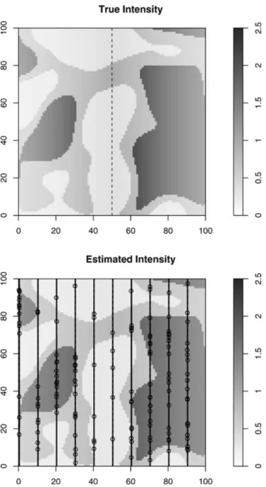
Figure 1. Example simulated intensity surface (top) and es-timated (bottom) surface with habitat and river feature and

K = 10,¯g= 0.25, P= 4%, and E(n) = 75.

average across all scenarios was 0.9% and 0.08% forE(n) = 75 and 400, respectively. We expect that any small amount of bias that does exist would occur from the resolution of the quadrature points for integration. Figure 1 illustrates that even with sparse transect sampling, informative gridded en-vironmental covariates can lead to an accurate prediction of intensity over the entire region with a known model.

The confidence interval coverage for the homogeneous Pois-son scenarios was within the expected range for both the CDS and model-based (IPP) estimators (Figure 2). For the IPP scenarios without overdispersion, the confidence interval cov-erage for the model-based estimator was within the expected

range but the observed coverage for CDS was too high ex-cept for the case with small sample size (E(n) = 75) and larger number of lines (K = 20). When overdispersion was added, the observed coverage was even higher for CDS. For the model-based estimator the ad hoc adjustment for overdis-persion was not sufficient and coverage was too low except with the larger number of lines (K = 20) and 4% sampling coverage. For most real applications, sampling coverage is less than 4%, so the ad hoc adjustment may be adequate as long asKis sufficiently large.

The average estimated coefficient of variation for the CDS-O1 variance estimator was 24% larger than the coefficient of variation for the model-based estimator for the IPP pro-cess without overdispersion. This reflected the bias in the es-timated standard error for CDS-O1, which was 23% larger than the standard deviation of the replicate values ofμ(A). The CDS-O1 variance estimator provided a reduction of 25% in comparison to the CDS-R2 estimator but was still larger than the true variance. Thus, as long as overdispersion can be accommodated, the model-based estimator can provide sub-stantial gains in precision in comparison to CDS even with the more recently developed systematic variance estimators. 4.2 Application to the Dubbo Weed Data

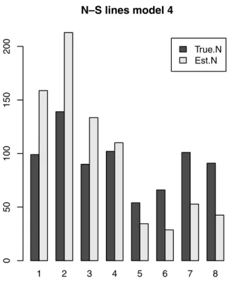
Melville and Welsh (2001) collected and analyzed line transect sampling data withn = 479 observed devil’s claw weeds in a farming paddock from eight 150 m wide parallel transects. These data are analyzed here as an example because the en-tire population was enumerated and the data highlight prob-lems that can occur in some unusual circumstances. Melville and Welsh (2001) stated that signed perpendicular distance (zk(s)) and the distance along each transect were measured;

however, only the signed perpendicular distances were pro-vided and they make no mention of the transect length in their paper. To analyze these data in a spatial context we have assumed that the paddock was square (1200 m by 1200 m) and we generated a restricted random uniformsy coordinate

for each object such that no weeds had the exact same coor-dinate. There were 742 weeds in the paddock with 99, 136, 90, 102, 54, 66, 101, and 91 in transects 1–8, respectively (Melville and Welsh, 2001). They stated that sheep were only present on transects 5–8 and they ate the leafy part of the weed so they expected that the weeds would be harder to detect on those transects. Using the known positions of all weeds and the observed weeds, we can describe the actual distribution of all perpendicular distances and the propor-tion detected within intervals of distance for transects with sheep absent and present (Table 1). Detection probability was slightly lower where sheep were present, but also the frequency of perpendicular distances decreased with distance where sheep were absent and increased with distance where sheep were present. This resulted in declining numbers ob-served with distance where sheep were absent and a roughly constant number observed for each interval where sheep were present.

We fitted models in which weed intensity differed (1) for sheep absence/presence, (2) for each of the eight strips, and (3) as a thin-plate regression spline (Wood, 2006) of the east– west coordinatesx. We modeled detection probability within

Model-Based Approach for Making Ecological Inference 315 E(n)=75 k=10 E(n)=75 k=20 E(n)=400 k=10 E(n)=400 k=20 E(n)=75 k=10 E(n)=75 k=20 E(n)=400 k=10 E(n)=400 k=20 CDS IPP 0.75 0.85 0.95 Coverage=4% HPP E(n)=75 k=10 E(n)=75 k=20 E(n)=400 k=10 E(n)=400 k=20 E(n)=75 k=10 E(n)=75 k=20 E(n)=400 k=10 E(n)=400 k=20 CDS IPP 0.75 0.85 0.95 Coverage=50% HPP E(n)=75 k=10 E(n)=75 k=20 E(n)=400 k=10 E(n)=400 k=20 E(n)=75 k=10 E(n)=75 k=20 E(n)=400 k=10 E(n)=400 k=20 CDS IPP 0.75 0.85 0.95 Coverage=4% IPP no overdispersion E(n)=75 k=10 E(n)=75 k=20 E(n)=400 k=10 E(n)=400 k=20 E(n)=75 k=10 E(n)=75 k=20 E(n)=400 k=10 E(n)=400 k=20 CDS IPP 0.75 0.85 0.95 Coverage=50% IPP no overdispersion E(n)=75 k=10 E(n)=75 k=20 E(n)=400 k=10 E(n)=400 k=20 E(n)=75 k=10 E(n)=75 k=20 E(n)=400 k=10 E(n)=400 k=20 CDS IPP 0.75 0.85 0.95 Coverage=4% IPP high overdispersion

E(n)=75 k=10 E(n)=75 k=20 E(n)=400 k=10 E(n)=400 k=20 E(n)=75 k=10 E(n)=75 k=20 E(n)=400 k=10 E(n)=400 k=20 CDS IPP 0.75 0.85 0.95 Coverage=50% IPP high overdispersion

Figure 2. Confidence interval coverage (nominal 95%) for 1825 replicates with the IPP and CDS-O1 estimators for each scenario with ¯g= 0.25. Results for ¯g= 0.60 were very similar. Vertical bars show expected range of simulation error.

Table 1

Known number of weeds(N) and the proportion(p)and number(n)observed in10equal distance bins for transects1–4 (sheep absent)and transects5–8 (sheep present)

Sheep [0,7.5] (7.5,15] (15,22.5] (22.5,30] (30,37.5] (37.5,45] (45,52.5] (52.5,60] (60,67.5] (67.5,75] Absent N 57 90 32 43 37 49 54 27 11 30 p 1.00 0.97 1.00 0.81 0.86 0.86 0.63 0.37 0.18 0.33 n 57 87 32 35 32 42 34 10 2 10 Present N 11 21 16 17 36 48 46 49 31 37 p 1.00 0.81 0.75 0.76 0.50 0.42 0.35 0.31 0.26 0.22 n 11 17 12 13 18 20 16 15 8 8

and considered a model with constantαand another in which

αdiffered based on sheep presence and absence. The model with minimum AIC included a separate α for sheep pres-ence/absence and intensity varying across strips (Table 2). The known population size was within one standard error of the estimated value of 774. However, the model was un-able to reflect the true spatial distribution of weeds across the paddock (Figure 3). The estimated number of weeds in transects 1–4 (sheep absent) were too high and the estimates were too low for transects 5–8 (sheep present). This occurred because the true spatial intensity was not constant within the strips and it varied based on presence of sheep. The esti-mated value ˆαwas 23.6 where sheep were absent and was sub-stantially larger at 56.5 where sheep were present. The latter

value should have been smaller because detection probability declined more rapidly where sheep were present. This is ap-parent by examining the observed and expected distributions for perpendicular distance (Figure 4). Using the distance bins in Figure 4 instead of transects, aχ2 _{statistic can be} calcu-lated as in equation (7). There is a substantial lack of fit (χ2₌ 51.5,df = 10,p <0.001) and the residuals reflect the increas-ing frequency of weeds with distance for transects with sheep present. The distance bin calculated ˆcapproximately doubles the standard errors for the abundance estimates in Table 2.

Even though the modeled intensity surface showed substan-tial lack of fit in an absolute (but not qualitative) sense, we chose the Dubbo data to illustrate not only the ability to compare environmental treatments with the IPP method, but

Table 2

Models fitted to Dubbo weed data and resulting estimates and precision of weed abundance in the entire paddock

Intensitya _{Detection # parameters ΔAIC N}ˆ _{Std. error}

∼Sheep ∼1 3 38.1 755 46 ∼Sheep ∼Sheep 4 15.8 773 47 ∼Strip ∼1 9 22.4 755 46 ∼Strip ∼Sheep 10 0.0 774 47 ∼s(x) ∼1 11 18.9 760 47 ∼s(x) ∼Sheep 12 5.2 769 47

a_{s(x) denotes thin-plate regression spline model.}

1 2 3 4 5 6 7 8 True.N Est.N

N–S lines model 4

Figure 3. True (dark) and estimated (light) number of weeds in each strip using the minimum AIC model for the Dubbo weed data.

also the ability to explore where or why a hypothesized rela-tionship may not fit as expected. We refrain from speculation here, but a researcher using this data can now explore the lack of fit and possibly look for other covariates which might be associated with this discrepancy. Certainly sheep presence is not enough to fully explain abundance patterns in this data. 5. Discussion

Casting distance sampling into a full likelihood formulation for the spatial point process and the observation process (de-tection) provides a natural model selection framework to eval-uate impacts of ecological processes and experimental manip-ulations (e.g., grazing) on animal abundance and distribution. Simultaneous fitting of the detection function copes with the potential influence of those same ecological variables and oth-ers (e.g., observer) on the point process parameter estimates

(0,7.5] (15,22.5] (37.5,45] (60,67.5] Sheep absent 02 0 6 0 (0,7.5] (15,22.5] (37.5,45] (60,67.5] Sheep present 05 1 5

Figure 4. Observed (light) and expected (dark) numbers of weeds in perpendicular distance intervals for transects with sheep absent and present.

and uncertainty resulting from the estimation of the detection parameters.

Use of this model-based approach does not require random transect placement so it will work as well with systematic de-signs, platforms of opportunity, and more optimal designs that are not restricted to designs with transects parallel to the den-sity gradient. However, some degree of caution is warranted and design considerations cannot be completely ignored. It is possible to pose models in which the detection parame-ters are completely confounded with the intensity parameparame-ters. For example, a model in which the underlying point process is a symmetric function of the perpendicular distance from the line is completely confounded with the detection process. Confounding of detection probability and intensity with this model-based approach can be avoided in a variety of ways. Melville and Welsh (2001) proposed estimation of detection from a calibration strip in which all objects were delineated and detection or nondetection was determined for each object. Detection probability would then be assumed to be constant across all of the strips. This is a rather strong assumption and the method would be impractical and inefficient in most situations. An alternative and more efficient approach would be a pattern of perpendicular strips as described by Buckland et al. (2007), which would enable detection of objects in both thesx andsy directions with certainty. Another alternative is

to survey with two independent observers allowing detection probability to be independently assessed with the capture– recapture data (Laake and Borchers, 2004; Borchers et al., 2006). This latter approach was used in migration counts of gray whales (Buckland, Breiwick, et al., 1993) in which the true offshore distribution (intensity) is confounded with the detection process in the context of distance sampling. Alter-natively, aerial surveys perpendicular to shore could be used to model the intensity process as a function of distance from

Model-Based Approach for Making Ecological Inference 317 shore which would eliminate any confounding as suggested by

Buckland et al. (2007).

Models for the spatial point process can be limited to use spatial coordinates like the one-dimensional spline used in the Dubbo weed example. Similar models can be created to pro-vide a smooth two-dimensional surface for the point process intensity. However, many practitioners will want to include habitat covariates or experimental treatments and such mod-els can be easily created. There is one drawback in using spa-tial covariates when the goal is estimation of total abundance. Unlike design based methods, the spatial covariates need to be known for the entire region and not just in the sampled region. Sometimes specifying the spatial covariates is a triv-ial exercise like the sheep treatment in the Dubbo weed data example. But in most cases, the spatial covariate values will need to be defined from a raster grid applied to layers of a geographical information system. The tools needed to manip-ulate geographical information system layers are available as packages for theR statistical software (R Development Core Team, 2008) that can be integrated with theDSpatpackage. There are two nontrivial extensions to the present work that would enhance the model-based method. First, our ad hoc approach for overdispersion is admittedly not a perfect solution because it will depend on the choice of scale and is limited by the degrees of freedom which can be nonpositive if too many parameters are fitted. The computationally inten-sive approach of Waagepetersen and Schweder (2006) is also limited by scale and can only measure overdispersion at the level of half of the transect width as well as requiring a Cox process model be specified. A potential modification would be to use a one-dimensionalK-function along the line to increase the potential scale for overdispersion measurement. Second, extensions of this work to include marked point processes would be useful for handling animals in groups (e.g., pods, flocks, or herds) and to examine species interactions. Using Markov point process models might be useful for this case. Markov models can be fitted using a pseudo-likelihood func-tion with little change to equafunc-tion (3). If ecological inference is the primary goal, then this may suffice; however, it is non-trivial to incorporate interaction into abundance estimation. The same is true of the Cox process. Clearly, this is an area that needs further research.

6. Supplementary Material

The Web Appendix referenced in Section 3.1 is available un-der the Paper Information link at the Biometrics website

http://www.biometrics.tibs.org.

Acknowledgements

The authors thank G. Melville for providing the Dubbo weed data and A. Baddeley for questions and modification of the

spatstatpackage. The authors also thank A. Zerbini and R. Hobbs for initial review of the article.

References

Baddeley, A. and Turner, R. (2000). Practical maximum pseudolikeli-hood for spatial point patterns.Australian & New Zealand Jour-nal of Statistics42,283–322.

Baddeley, A. and Turner, R. (2005).Spatstat: AnRpackage for ana-lyzing spatial point patterns.Journal of Statistical Software12,

1–42.

Berman, M. and Turner, T. R. (1992). Approximating point process likelihoods with GLIM.Applied Statistics41,31–38.

Borchers, D. L., Buckland, S. T., Goedhart, P. W., Clarke, E. D., and Hedley, S. L. (1998). Horvitz-Thompson estimators for double-platform line transect surveys.Biometrics54,1221–1237. Borchers, D. L., Laake, J. L., Southwell, C., and Paxton, C. G.

M. (2006). Accommodating unmodeled heterogeneity in double-observer distance sampling surveys.Biometrics62,372–378. Buckland, S. T., Anderson, D. R., Burnham, K. P., and Laake, J. L.

(1993).Distance Sampling: Estimating Abundance of Biological Populations. London: Chapman & Hall.

Buckland, S. T., Breiwick, J. M., Cattanach, K. L., and Laake, J. L. (1993). Estimated population size of the California gray whale. Marine Mammal Science9,235–249.

Buckland, S. T., Anderson, D. R., Burnham, K. P., Laake, J. L., Borchers, D. L., and Thomas, L. (2001).Introduction to Distance Sampling: Estimating Abundance of Biological Populations. New York: Oxford University Press.

Buckland, S. T., Anderson, D. R., Burnham, K. P., Laake, J. L., Borchers, D. L., and Thomas, L. (2004). Advanced Distance Sampling: Estimating Abundance of Biological Populations. New York: Oxford University Press.

Buckland, S. T., Borchers, D. L., Johnston, A., Henrys, P. A., and Marques, T. A. (2007). Line transect methods for plant surveys. Biometrics63,989–998.

Burnham, K. P. and Anderson, D. R. (2002).Model Selection and Mul-timodel Inference: A Practical Information-theoretic Approach. New York: Springer-Verlag Inc.

Cox, D. R. (1955). Some statistical methods related with a series of events.Journal of the Royal Statistical Society, Series B17,129– 157.

Cressie, N. A. C. (1993).Statistics for Spatial Data. New York: John Wiley & Sons.

Dawson, S. E., Slooten, S., DuFresne, S., Wade, P., and Clement, D. (2004). Small-boat surveys for coastal dolphins: line-transect surveys for Hector’s dolphins (Cephalorhynchus hectori).Fishery Bulletin102,441–451.

Diggle, P. J. (2003).Statistical Analysis of Spatial Point Patterns, 2nd edition. London: Academic Press.

Dorfman, R. (1938). A note on the delta-method for finding variance formulae.The Biometric Bulletin1,129–137.

Eberhardt, L. L. (1967). Some developments in “distance sampling.” Biometrics23,207–216.

Fewster, R. M., Buckland, S. T., Burnham, K. P., Borchers, D. L., Jupp, P. E., Laake, J. L., and Thomas, L. (2009). Estimating the encounter rate variance in distance sampling.Biometrics65,

225–236.

Guan, Y. and Loh, J. M. (2007). A thinned block bootstrap variance estimation procedure for inhomogeneous spatial point patterns. Journal of the American Statistical Association102,1377–1386. Hedley, S. L. and Buckland, S. T. (2004). Spatial models for line tran-sect sampling.Journal of Agricultural, Biological, and Environ-mental Statistics9,181–199.

Innes, S., Heide-Jorgensen, M. P., Laake, J. L., Laidre, K. L., Cleator, H. J., Richard, P., and Stewart, R. E. A. (2002). Surveys of bel-ugas and narwhals in the Canadian high Arctic in 1996. In Bel-ugas in the North Atlantic and the Russian Arctic, M. P. Heide-Jorgensen and O. Wiig (eds), volume 4 ofNAMMCO Scientific Publications, 169–190. Tromso, Norway: North Atlantic Marine Mammal Commission.

Laake, J. L. and Borchers, D. L. (2004). Methods for incomplete detection at distance zero. In Advanced Distance Sampling,

S. Buckland, D. Anderson, K. Burnham, J. Laake, D. Borchers, and L. Thomas (eds), 108–189. New York: Oxford University Press.

Laake, J. L., Guenzel, R. J., Bengtson, J. L., Boveng, P. L., Cameron, M., and Hanson, M. B. (2008). Coping with variation in aerial survey protocol for line transect sampling.Wildlife Research35,

289–298.

Marques, F. F. C. and Buckland, S. T. (2003). Incorporating covariates into standard line transect analyses.Biometrics59,924–935. McCullagh, P. and Nelder, J. (1989).Generalized Linear Models, 2nd

edition. Boca Raton, Florida: Chapman & Hall/CRC.

Melville, G. J. and Welsh, A. H. (2001). Line transect sampling in small regions.Biometrics57,1130–1137.

Møller, J. and Waagepetersen, R. (2003).Statistical Inference and Sim-ulation for Spatial Point Processes. Boca Raton, Florida: Chap-man & Hall/CRC.

Nayak, T. K. (2002). Rao-Cramer type inequalities for mean square error prediction.American Statistician56,102–106.

R Development Core Team. (2008). R: A language and environ-ment for statistical computing. Vienna, Austria: R Foundation for Statistical Computing. ISBN 3–900051-07–0. http://www.R-project.org, accessed April 23, 2009.

Ramsey, F. L. and Harrison, K. (2004). A closer look at detectability. Environmental and Ecological Statistics11,73–84.

Royle, J. A., Dawson, D. K., and Bates, S. (2004). Modeling abundance effects in distance sampling.Ecology85,1591–1597.

Schlather, M. (2001). Simulation of stationary and isotropic random fields.R News1,18–20.

Schweder, T. (1977). Point process models for line transect experiments. InRecent Developments in Statistics, J. R. Barra, B. Van Cutsem, F. Brodeau, and G. Romier (eds), 221—242. Amsterdam: North Holland.

Skaug, H. (2006). Markov modulated Poisson processes for clustered line transect data.Environmental and Ecological Statistics 13,

199–211.

Thomas, L., Laake, J. L., Strindberg, S., Marques, F. F. C., Buckland, S. T., Borchers, D. L., Anderson, D. R., Burnham, K. P., Hedley, S. L., Pollard, J. H., Bishop, J. R. B., and Marques, T. A. (2006). Distance 5.0. U.K.: Research Unit for Wildlife Population Assess-ment, University of St. Andrews.http://www.ruwpa.st-and. ac.uk/distance/, accessed April 23, 2009.

Vidal, O., Barlow, J., Hurtado, L. A., Torre, J., Cendon, P., and Ojeda, Z. (1997). Distribution and abundance of the Amazon river dolphin (i nia geoffrensis) and the tucuxi (sotalia fluviatilis) in the Upper Amazon river.Marine Mammal Science13,427– 445.

Waagepetersen, R. and Schweder, T. (2006). Likelihood-based in-ference for clustered line transect data. Journal of Agri-cultural, Biological, and Environmental Statistics 11, 264– 279.

Wood, S. N. (2006).Generalized Additive Models: An introduction with R. Boca Raton, Florida: Chapman and Hall/CRC.

Received July2008.Revised January2009.