Improved Binary Similarity Measures for Software Modularization

(1)

Frontiers of Information Technology & Electronic Engineering www.zju.edu.cn/jzus; engineering.cae.cn; www.springerlink.com ISSN 2095-9184 (print); ISSN 2095-9230 (online)

E-mail: [email protected]

Improved binary similarity measures for

software modularization

⇤

Rashid NASEEM†1_{, Mustafa Bin Mat DERIS}1_{, Onaiza MAQBOOL}2_,

Jing-peng LI3_{, Sara SHAHZAD}4_{, Habib SHAH}5

(1_{Faculty of Computer Science and Information Technology,Universiti Tun Hussein Onn Malaysia, Malaysia)}

(2_{Department of Computer Science, Quaid-i-Azam University, Islamabad, Pakistan)}

(3_{Division of Computer Science and Mathematics, University of Stirling, UK)}

(4_{Department of Computer Science, University of Peshawar, Peshawar, Pakistan)}

(5_{Faculty of Computer and Information Systems, Islamic University Madina, KSA)}

†_{E-mail: [email protected]}

Received Oct. 30, 2015; Revision accepted Apr. 12, 2016; Crosschecked

Abstract: Various binary similarity measures have been employed in clustering approaches to make homogeneous groups of similar entities in the data. These similarity measures are mostly based only on the presence and absence of features. Binary similarity measures have also been explored with diﬀerent clustering approaches (e.g., agglomerative hierarchical clustering) for software modularization to make the software systems understandable and manageable. Each similarity measure has its own strengths and weaknesses that result in improving and deteriorating the clustering results, respectively. This paper highlights the strengths of some well-known existing binary similarity measures for software modularization. Furthermore, based on these existing similarity measures, this paper introduces the improved new binary similarity measures. Proofs of the correctness with illustration and a series of experiments are presented to evaluate the eﬀectiveness of our new binary similarity measures.

Key words: Binary similarity measure, Binary features, Combination of measures, Software modularization http://dx.doi.org/10.1631/FITEE.1500373 CLC number:

1 Introduction

Clustering is an approach that makes clusters of similar entities in the data. Entities in a cluster are similar to each other (based on characteristics or fea-tures) while they are distinct from entities in other clusters. In the software domain, an important appli-cation of clustering is to modularize a software sys-tem or to recover the module architecture or compo-nents of the software systems by clustering the

soft-*_{Project supported by the O}_ﬃ_{ce of Research, Innovation,}

Com-mercialization and Consultancy Oﬃce (ORICC), Universiti Tun Hussein Onn Malaysia (UTHM) (No. U062)

ORCID: Rashid NASEEM, http://orcid.org/0000-0002-4952-8100

cZhejiang University and Springer-Verlag Berlin Heidelberg 2016

ware entities, for example, functions, files or classes, in the source code. Recovery is very important when no up-to-date documentation of a software system is available (Shtern and Tzerpos, 2014). Besides clustering, other approaches have also been used for software modularization, for example, super-vised clustering (Hallet al., 2012), optimization tech-niques (Praditwonget al., 2011), role-based recovery (Dugerdil and Jossi, 2008), graph-based techniques (Bittencourt and Guerrero, 2009), association-based approaches (Vasconcelos and Werner, 2007), spec-tral method (Xanthos and Goodwin, 2006), rough set theory (Jahnke, 2004), concept analysis (Tonella, 2001), and visualization tools (Synytskyy et al., 2005).

(2)

A key activity in software clustering consists of gathering the entities from source code of software systems into meaningful and independent modules. The process of software clustering usually starts with the selection of entities and their features by parsing the source code of software systems. Then entities are organized into cohesive clusters by employing a particular clustering algorithm (Mitchell and Man-coridis, 2006).

Agglomerative Hierarchical Clustering (AHC) algorithms have been widely used by researchers to cluster the software systems (Muhammad et al., 2012) (Maqbool and Babri, 2007) (Patelet al., 2009) (Shtern and Tzerpos, 2010) (Mitchell, 2006) (An-quetil and Lethbridge, 1999) (Wiggerts, 1997). AHC comprises two main factors, a similarity measure to find the association between two entities and a link-age method to update the similarity values between entities in each iteration. However, selection of a sim-ilarity measure is an important factor in AHC (Cui and Chae, 2011) (Jackson et al., 1989), which has a major influence on the clustering results (Naseem

et al., 2010) (Shtern and Tzerpos, 2012).

There exist a large number of binary similarity measures (Choiet al., 2010) (Cheetham and Hazel, 1969). Nevertheless, for software modularization, the comparative studies have reported that Jaccard (JC) binary similarity measure produced better clus-tering results (Tzerpos and Holt, 2000) (Davey and Burd, 2000) (Lunget al., 2004) (Shtern and Tzerpos, 2012). In our previous study (Naseemet al., 2010), we proposed a new binary similarity measure, called JaccardNM (JNM), which could overcome some de-ficiencies of the JC binary similarity measure. We also examined the Russell&Rao (RR) binary simi-larity measure for software modularization for the first time, and found that it could generate better results as compared to JC and JNM binary similar-ity measures for some of the test software systems. In another study (Naseemet al., 2013), we proposed COUSM (Cooperative Only Update Similarity Ma-trix) clustering algorithm, which combines two sim-ilarity measures in a single clustering process based on AHC.

In this paper, we explore the integration of the existing binary similarity measures for AHC algo-rithms using linkage methods (e.g., Complete Link-age (CL), Single LinkLink-age (SL) and Weighted AverLink-age Linkage (WL) methods). For example, we select the

JC similarity measure, which produces a relatively large number of clusters (Maqbool and Babri, 2004) (Saeed et al., 2003) and the JNM binary similar-ity measure, which takes a less number of arbitrary decisions (Naseem et al., 2010) during the cluster-ing process. Durcluster-ing the clustercluster-ing process, creatcluster-ing a large number of clusters means that a clustering approach may create compact clusters, hence im-proving the quality of clustering results (Maqbool and Babri, 2007). Arbitrary decision is the arbitrary clustering of two entities when there exist more than two equally similar entities; hence, arbitrary deci-sions create problems and reduce the quality of clus-tering results (Naseem et al., 2010) (Maqbool and Babri, 2007). This analysis leads us to introduce better binary similarity measures by combining the JC and JNM measures.

This study mainly focuses on the identification of the strengths of the existing binary similarity mea-sures.Moreover, the improved similarity measures are based on the integration of JC, JNM, and RR similarity measures. While in our previous studies (Naseemet al., 2010) (Naseemet al., 2011), the main focus was to explore the deficiencies (i.e., creating a large number of equal similarity values and giving no importance to a pair of entities sharing a large number of features) of some well-known binary simi-larity measures and then solved these deficiencies by adding the total proportion of features to the denom-inator in the JC similarity measure.

The contributions of this paper can be summa-rized as:

1. Analysis of the Jaccard and JaccardNM (Naseem et al., 2010) similarity measures for binary features and a comparison of their strengths;

2. The integration of the strengths of existing bi-nary similarity measures to form new bibi-nary similarity measures for software clustering; 3. Introduction of four improved binary

similar-ity measures that yield more eﬀective solutions than the existing binary similarity measures. They are as follows:

(a) JCJNM: add the JC and JNM binary sim-ilarity measures;

(b) JCRR: add the JC and RR binary similar-ity measures;

(3)

(c) JNMRR: add the JNM and RR binary sim-ilarity measures;

(d) JCJNMRR: add the JC, JNM and RR bi-nary similarity measures.

4. The additional evidence providing support to the correctness of the new binary similarity mea-sures;

5. Conducting an experimental study that presents an external and internal evaluation of the pro-posed and existing similarity measures.

6. For all evaluation criteria, on average, our new similarity measures outperform the existing sim-ilarity measures.

The rest of this paper is organized as follows: Section 2 presents the preliminaries of software mod-ularization using AHC algorithms. The strengths of the existing similarity measures are presented and illustrated in Section 3. This section also gives the derivations of our new similarity measures with proofs of correctness. Section 4 presents the exper-imental setup, which lists all the test software sys-tems, similarity measures, linkage methods and eval-uation criteria that are used to perform the series of experiments. Section 5 gives the experimental re-sults and discussion on comparing our new similarity measures with existing similarity measures by using diﬀerent external and internal criteria. Section 6 concludes this paper.

2 Software Modularization Using AHC

Clustering algorithms can be broadly catego-rized into hierarchical and partitional. As stated in Section 1, AHC has been commonly used for software modularization. AHC considers each entity to be a singleton cluster and groups the two most similar clusters at every step. At the end, it makes one large cluster, which contains all the entities, as shown in Algorithm 1.

Partitional clustering produces flat clusters with no hierarchy, and requires prior knowledge of the number of clusters. In the software domain, parti-tional clustering has also been used (Kanellopoulos

et al., 2007) (Lakhotia, 1997) (Shah et al., 2013); however, there are some advantages of using AHC.

Algorithm 1- Agglomerative Hierarchical Cluster-ing (AHC) Algorithm

Input: Feature (F) matrix

Output: Hierarchy of Clusters (Dendrogram)

1: Create a similarity matrix by calculating similarity using aSimilarity Measurebetween each pair of entities 2: repeat

3: Group the most similar (singleton) clusters into one cluster (using maximum value of similarity in similarity matrix)

4: Update the similarity matrix by recalculating similar-ity using a Linkage Methodbetween newly formed cluster and existing (singleton) clusters

5: until the required number of clusters or a single large cluster is formed

For example, AHC does not require prior informa-tion about the number of clusters. Moreover, Wig-gerts (1997) stated that the process of AHC is very similar to the approach of reverse engineering where architecture of a software system is recovered in a bottom-up fashion. AHC provides diﬀerent levels of abstraction and can be useful for end users to select the desired number of clusters when the modulariza-tion results are meaningful to them (Lutellieret al., 2015). Since a maintainer may not have the knowl-edge of the number of clusters in advance, therefore viewing the architecture at diﬀerent abstraction lev-els facilitates understanding. Techniques have also been proposed to select an appropriate abstraction level, for example, (Chonget al., 2013) proposed a dendrogram cutting approach for this purpose.

When AHC is utilized for software modulariza-tion, the first step that occurs is the selection of the entities to be clustered where each entity is described by diﬀerent features. The steps are presented in more detail in the following subsections.

2.1 Selection of Entities and Features

Selecting the entities and features associated with entities depends on the type of software system and the desired architecture (e.g., layered/module architectures) to be recovered. For software mod-ularization, researchers have used diﬀerent types of entities, for example, methods (Saeed et al., 2003), classes (Bauer and Trifu, 2004) and files (Andrit-sos and Tzerpos, 2005), (Anquetil and Lethbridge, 1999). Researchers have also used diﬀerent types of features to describe the entities such as global vari-ables used by an entity (Muhammad et al., 2012), and procedure calls (Andritsos and Tzerpos, 2005).

(4)

Features are based on the relationships between enti-ties, for example, containment and inheritance. Fea-tures may be in the binary or non-binary format. A binary feature represents the presence or absence of a relationship between two entities, while non-binary features are weighted features using diﬀerent weight-ing schemes, for example, absolute and relative (Cui and Chae, 2011), to demonstrate the strength of the relationship between entities. Binary features are widely used in software modularization (Cui and Chae, 2011) (Mitchell and Mancoridis, 2006) (Wig-gerts, 1997).

To apply AHC, a software system must be parsed to extract the selected entities and features associated with entities. This process results in a feature matrix of size N x P, where N is the total number of entities andP is the total number of fea-tures. Each entity in the feature matrix has a feature vector fi, fi = {f1, f2, f3, ..., fP}. More generally,F

presents a general feature matrix, which takes values from {0,1}p_{; in other words,}_F _{= {0,1}}p_{, where ‘1’} means presence of a feature and ‘0’ otherwise. AHC takesF as input, as shown in Algorithm I. Table 1 shows an example feature matrixF of a very small imaginary software system, which contains 5 entities (E1-E5) and 7 binary features (f1-f7). In Table 1, for example, f1 is present in entities E1, E2, and E3 while absent in entities E4 and E5.

Table 1 An Example Feature (F) Matrix f1 f2 f3 f4 f5 f6 f7 E1 1 1 0 0 0 0 0 E2 1 1 0 0 0 0 0 E3 1 0 1 1 0 0 0 E4 0 0 1 1 1 0 0 E5 0 0 0 0 0 1 0

2.2 Selection of Similarity Measure

The first step of the AHC process is to calculate the similarity between each pair of entities to obtain a similarity matrix by using a similarity measure, as shown in Step 1 of Algorithm I. Following are some well-known binary similarity measures for software modularization. Jaccard(JC) = a a+b+c (1) JaccardN M(JNM) = a 2(a+b+c) +d (2) Russell&Rao(RR) = a a+b+c+d (3) All the existing binary similarity measures are expressed as functions of the following four quantities associated with the pair of entities (Ei, Ej),8Ei, Ej

2F (Lesot and Rifqi, 2009):

• the number of features common to both entities, denoted bya

• the number of features present in Ei, but not in Ej, denoted byb

• the number of features present in Ej, but not in Ei, denoted byc

• the number of features absent in both entities, denoted byd.

It is important to note thata+b+c+d is a con-stant value and is equal to the total number of fea-turesP.a+b=0occurs only when Ei has the feature vector fi = (0,...,0). Likewise, a+c=0 shows that Ej has feature vector fj = (0,...,0).

Definition 1 A binary similarity measure,SM, is a function whose domain is {0,1}p_{, and whose range} isR+_{, that is,}_SM _{: {0,1}}p

!R+_{(Veal, 2011), with}

the following properties:

• Positivity:SM(Ei,Ej) 0,8Ei, Ej2F

• Symmetry: SM(Ei,Ej)=SM(Ej,Ei),₈Ei, Ej₂

F

• Maximality: SM(Ei,Ei) SM(Ei,Ej),8 Ei, Ej 2F

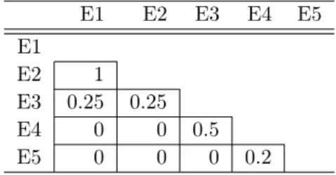
Table 2 The similarity matrix derived from the ma-trix in Table 1 by using the JC similarity measure

E1 E2 E3 E4 E5 E1 E2 1 E3 0.25 0.25 E4 0 0 0.5 E5 0 0 0 0.2

To illustrate the calculation, for instance, of the JC measure as defined in Equation 1, Table 2 gives

(5)

the similarity matrix of the feature matrix shown in Table 1. The similarity between E1 and E2 is cal-culated using the quantities defined by a, b, c, and d, and in this case a = 2, b = 0, c = 0, and d = 5. Putting all these values in JC similarity measure, we get similarity value ‘1’ (shown in Table 2). Likewise, similarity values are calculated for each pair of en-tities and are presented in Table 2. Now AHC will group the most similar entities in Table 2, accord-ing to the Step 2 in Algorithm I. E1 and E2 have the highest similarity value, so AHC groups these entities in a single cluster (E1E2). A new cluster is therefore formed, and AHC will update the similar-ity values of E1E2 and all other (singleton) clusters, that is, E3, E4, and E5. To update these similarity values, diﬀerent linkage methods can be used, which are described in the next subsection.

2.3 Selection of the Linkage Method

When a new cluster is formed, the similarities between new and the existing clusters are updated using a linkage method, as shown in step 3 of Algo-rithm I. There exist a number of methods, which up-date similarities diﬀerently. However, in this study, we discuss only those methods that are widely used for software modularization. They are listed below, where (EiEj) represents a new cluster and Ek repre-sents an existing singleton cluster.

• Complete Linkage: CL(EiEj, Ek)= min(sim(Ei,

Ek), sim(Ej, Ek))

• Single Linkage: SL(EiEj, Ek)= max(sim(Ei, Ek), sim(Ej, Ek))

• Weighted Average Linkage:WL(EiEj, Ek)= 0.5 * (sim(Ei, Ek) + sim(Ej, Ek))

In the illustrative example, we update similarity values between a new cluster (E1E2) and existing singleton clusters using CL method. The updated similarity matrix is shown in Table 3. For example, the CL method returns the minimum similarity value between E1 and E3 (0.25) and E2 and E3 (0.25). Both of the returned values are the same (if there was a minimum, then that value would be selected). Therefore, AHC selects this similarity value as the new similarity between (E1E2) and E3, as shown in Table 3. Similarly, all similarity values are updated between (E1E2) and E4 and E5.

AHC repeats Steps 2 and 3 until all entities are merged in one large cluster, or the desired number of clusters is obtained. At the end, AHC results in a hierarchy of clusters, also known as dendrogram, which is shown for the current example in Figure 1. The obtained hierarchy is then evaluated to assess the quality of the automatically formed clusters, and the performance of similarity measures and methods.

2.4 Assessment of the Results

Assessment of the clustering results is usually carried out using two approaches: external and inter-nal assessment. The exterinter-nal assessment approach finds the association between automated results (de-composition) and the authoritative decomposition prepared by a human expert (e.g., original developer of the test software system). The approach is also known asAuthoritativeness. The automated position should resemble the authoritative decom-position as much as possible (Wuet al., 2005). To find the authoritativeness, diﬀerent measures may be used, such as, precision, recall (Sartipi and Konto-giannis, 2003), MoJo, and MoJoFM. Here, the widely used MoJoFM (Wen and Tzerpos, 2004) is discussed. MoJoFM is the updated version of the MoJo (Tzer-pos and Holt, 1999) (Tzer(Tzer-pos, 2003), which calcu-lates the move and join operations to convert the automated decomposition (M) into authoritative de-composition (N).

Table 3 The updated similarity matrix from the val-ues in Table 2 using CL linkage method

E1E2 E3 E4 E5 E1E2

E3 0.25

E4 0 0.5

E5 0 0 0.2

Fig. 1 Hierarchy created using the JC measure and CL method

(6)

M oJoF M(M, N) = ✓ 1 mno(M, N) max(mno(₈M, N)) ◆ ⇤100 (4) where mno(M, N) is the minimum number of ‘move’ and ‘join’ operations required to translateM in toN andmax(mno(₈M, N))is the maximum of mno(₈M, N). MoJoFM produces percentage of the similarity between two decompositions. A higher percentage shows greater correspondence between the two decompositions and hence better results, while lower percentage indicates that the decompo-sitions are diﬀerent.

Internal assessment is to evaluate the quality of the internal characteristics of the clusters in au-tomated decomposition. There exist a number of measures to evaluate the cluster quality internally, for example, arbitrary decisions (Wanget al., 2010), number of clusters (Wanget al., 2010), size of clus-ters (extremity) (Glorieet al., 2009), modularization quality (Praditwong, 2011), and coupling and cohe-sion (Cui and Chae, 2011). In this study, we intend to use arbitrary decisions and number of clusters. Ar-bitrary decisions are taken by AHC when there exist more than one maximum similarity values in the sim-ilarity matrix during iteration. Thus, the decision of selecting the maximum value is arbitrary, since more than one pair of entities is equally similar. A large number of arbitrary decisions shows poor character-istic of the clusters, while a less number of arbitrary decisions mean good characteristic, in terms of au-thoritativeness (Naseemet al., 2013). The number of clusters is another internal assessment criterion that is used to evaluate cluster quality. If an AHC produces a large number of clusters during the clus-tering process, it means that clusters are compact and have good quality (Maqbool and Babri, 2007). A less number of clusters during clustering means that they are large in size and less compact, and hence are considered poor quality.

3 New Similarity Measures

As discussed in Section 1, we define new simi-larity measures that have the combined strengths of existing similarity measures JC, JNM, and RR de-fined in Equations 1, 2 and 3, respectively. These three similarity measures have shown better results for software modularization as compared to other

measures (Cui and Chae, 2011). To highlight the strengths of these existing measures, we first present a small example case study, and then define our new similarity measures.

3.1 An Example Case Study

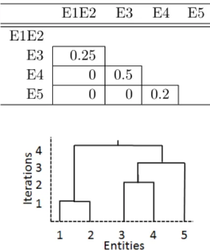
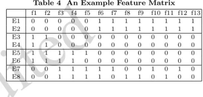
To illustrate the strengths of existing similarity measures, we take a small example of an imaginary feature matrix from (Naseemet al., 2013). The ex-ample feature matrix is shown in Table 4, with 8 enti-ties (E1–E8) and 13 features (f1–f13). Using feature matrix shown in Table 4, we illustrate the strengths of JC and JNM similarity measures. We use the CL method in AHC using the CL with JC and the CL with JNM on the feature matrix in Table 4.

Table 4 An Example Feature Matrix

f1 f2 f3 f4 f5 f6 f7 f8 f9 f10 f11 f12 f13 E1 0 0 0 0 0 1 1 1 1 1 1 1 1 E2 0 0 0 0 0 1 1 1 1 1 1 1 1 E3 1 1 0 0 0 0 0 0 0 0 0 0 0 E4 1 1 0 0 0 0 0 0 0 0 0 0 0 E5 1 1 1 1 1 0 0 0 0 0 0 0 0 E6 1 1 1 1 0 0 0 0 0 0 0 0 0 E7 0 0 1 1 1 1 1 0 0 1 0 1 0 E8 0 0 1 1 1 1 0 1 1 0 1 0 0

3.1.1 JC with CL clustering process

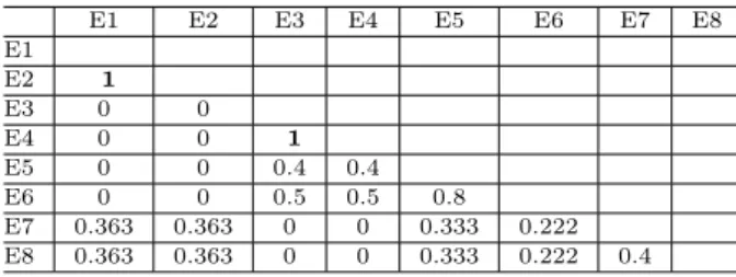
First, we illustrate the JC measure with the CL method. The first step of AHC is to create the sim-ilarity matrix using a simsim-ilarity measure. After ap-plying the JC measure to feature matrix in Table 4, we get the similarity matrix shown in Table 5. In the first iteration of AHC, a maximum similarity value from the similarity matrix (Table 5) is selected to make a new cluster or update a cluster. So, AHC searches for a maximum similarity value in Table 5 but it finds maximum similarity value ‘1’ twice (i.e., for (E1E2) and (E3E4)). AHC may select either, but we enforced AHC to select the last occurring value, that is, similarity value of (E3E4) (see Table 6).

The CL method is used to update the similarity values between the new cluster (E3E4) and all ex-isting singleton clusters, and the updated similarity matrix is shown in Table 6. In the second iteration, AHC searches again for the maximum value in up-dated similarity matrix Table 6. This time it makes (E1E2) as a new cluster and updates its similarity values with all other existing clusters, as shown in Table 7. In iterations 3 and 4, it makes clusters of (E5E6) and (E7E8), as shown in Table 8 and Table

(7)

9, respectively. From Table 8, it can be seen that there are two maximum values (0.4), hence AHC may select either again. As stated earlier, AHC will select a value that occurs later; therefore, it a makes cluster (E7E8). In the remaining iterations, AHC makes clusters of ((E3E4)(E5E6)), ((E1E2)(E7E8)) and (((E1E2) (E7E8)) ((E3E4) (E5E6))), as shown in Tables 10–12.

Table 5 Similarity matrix of table 4 using the Jaccard (JC) similarity measure E1 E2 E3 E4 E5 E6 E7 E8 E1 E2 1 E3 0 0 E4 0 0 1 E5 0 0 0.4 0.4 E6 0 0 0.5 0.5 0.8 E7 0.363 0.363 0 0 0.333 0.222 E8 0.363 0.363 0 0 0.333 0.222 0.4

Table 6 Iteration 1: updated similarity matrix of Table 5 using the CL method

E1 E2 (E3E4) E5 E6 E7 E8 E1 E2 1 (E3E4) 0 0 E5 0 0 0.4 E6 0 0 0.5 0.8 E7 0.363 0.363 0 0.333 0.222 E8 0.363 0.363 0 0.333 0.222 0.4

Table 7 Iteration 2: updated similarity matrix of Table 6 using the CL method

(E1E2) (E3E4) E5 E6 E7 E8 (E1E2) (E3E4) 0 E5 0 0.4 E6 0 0.5 0.8 E7 0.363 0 0.333 0.222 E8 0.363 0 0.33 0.222 0.4

3.1.2 JNM with the CL clustering process

Now we apply the JNM measure on the fea-ture matrix given in Table 4, and get a similarity matrix that can be seen in Table 13. The pro-cess for making clusters is the same as discussed in Subsection 3.1.1. As per the AHC, the first cluster formed is (E1E2), second is (E5E6), third is (E7E8), fourth is ((E1E2) (E7E8)), fifth is (E3E4), sixth is ((E3E4) (E5E6)), and the last is (((E1E2) (E7E8)) ((E3E4) (E5E6))). The similarity matrices during iterations—from the first iteration to the seventh (n-1) iteration—are given in Tables 14 to 20. In each

Table 8 Iteration 3: Updated Similarity Matrix of Table 7 Using the CL Method

(E1E2) (E3E4) (E5E6) E7 E8 (E1E2)

(E3E4) 0

(E5E6) 0 0.4

E7 0.363 0 0.222

E8 0.363 0 0.222 0.4

iteration, the CL method is used to update the simi-larity between newly formed and existing (singleton) clusters.

Fig. 2 Number of clusters and arbitrary decisions created by JC and JNM

(8)

(E1E2) (E3E4) (E5E6) (E7E8) (E1E2)

(E3E4) 0 (E5E6) 0 0.4 (E7E8) 0.363 0 0.2

(E1E2) ((E3E4)(E5E6)) (E7E8) (E1E2)

((E3E4)(E5E6)) 0

(E7E8) 0.363 0

((E1E2)(E7E8)) ((E3E4)(E5E6)) ((E1E2)(E7E8))

((E3E4)(E5E6)) 0

(((E1E2)(E7E8))((E3E4)(E5E6))) (((E1E2)(E7E8))((E3E4)(E5E6)))

Table 13 Similarity Matrix of Feature Matrix in Ta-ble 4 Using the JNM Similarity Measure

E1 E2 E3 E4 E5 E6 E7 E8 E1 E20.381 E3 0 0 E4 0 0 0.133 E5 0 0 0.111 0.111 E6 0 0 0.118 0.118 0.222 E7 0.166 0.166 0 0 0.136 0.09 E8 0.166 0.166 0 0 0.136 0.09 0.173

(E1E2) E3 E4 E5 E6 E7 E8 (E1E2) E3 0 E4 0 0.133 E5 0 0.111 0.111 E6 0 0.118 0.1180.222 E7 0.166 0 0 0.136 0.09 E8 0.166 0 0 0.136 0.09 0.173

(E1E2) E3 E4 (E5E6) E7 E8 (E1E2) E3 0 E4 0 0.133 (E5E6) 0 0.111 0.111 E7 0.166 0 0 0.09 E8 0.166 0 0 0.09 0.173

(E1E2) E3 E4 (E5E6) (E7E8) (E1E2)

E3 0

E4 0 0.133

(E5E6) 0 0.111 0.111 (E7E8) 0.166 0 0 0.09

((E1E2)(E7E8)) E3 E4 (E5E6) ((E1E2)(E7E8))

E3 0

E4 0 0.133

(E5E6) 0 0.111 0.111

((E1E2)(E7E8)) (E3E4) (E5E6) ((E1E2)(E7E8))

(E3E4) 0

(E5E6) 0 0.111

((E1E2)(E7E8)) ((E3E4)(E5E6)) ((E1E2)(E7E8))

((E3E4)(E5E6)) 0

(9)

3.1.3 Discussion on the results of JC and JNM mea-sures

In the previous two Subsections 3.1.1 and 3.1.2, we observed that the JC measure results in more clusters during clustering as compared to the JNM measure. Figure 2 shows the maximum number of clusters achieved and the total number of arbitrary decisions made during the clustering process for both measures. It can be seen from Figure 2 that the JNM measure produces a less number of arbitrary decisions as compared to the JC measure. The JNM produces results as expected because the main intu-ition of introducing this measure is to reduce the ar-bitrary decisions (Naseemet al., 2010). Hence, from these results we can easily conclude that the JC has the strength to create more clusters during the clus-tering process, while the JNM has the strength to reduce the number of arbitrary decisions.

It has been shown that if a clustering approach results in a large number of clusters during the clus-tering process, it increases the cohesiveness of the clusters and hence increases the authoritativeness of the results (Maqbool and Babri, 2007). Second, in our previous study, we showed that if a clustering approach reduces arbitrary decisions, it would cre-ate more authoritative results (Naseemet al., 2013). This analysis leads us to define the new measures that may have the characteristics of these existing similarity measures. It would be useful to integrate the existing similarity measures and come up with the new measures to increase the number of clusters and reduce the arbitrary decisions during the clus-tering process.

3.2 The New Binary Similarity Measures

According to the aforementioned discussion, the JC measure has the strength of creating a large num-ber of clusters during the clustering process, while the JNM measure has the strength of creating clus-ters with a less number of arbitrary decisions. We also consider the RR measure because for some case studies, it has produced better clustering results for software modularization (Naseemet al., 2010). RR reduces the arbitrary decisions when JC creates, for example, when the values ofaamong the entities are diﬀerent andb+c= 0. To combine the strengths of these existing similarity measures, the add operation is used to combine the existing similarity measures.

We introduce four new similarity measures as follows: 3.2.1 Addition of the JC and JNM measures: “JCJNM” similarity measure

The strengths of similarity measures shown in Subsection 3.1 can be combined by adding both the similarity measures (JC and JNM) to obtain the “JCJNM” binary similarity measure. Our new mea-sure“JCJNM” is defined as:

JCJN M =JC+JN M =a s+ a 2s+d =a(3s+d) s(2s+d) (5) where s=a+b+c

3.2.2 The Example Case Study and JCJNM Mea-sure

To demonstrate the strengths of our new mea-sure, we now apply the JCJNM similarity measure to the example feature matrix shown in Table 4. The corresponding similarity matrix using the JCJNM similarity measure is shown in Table 21. The CL method is used to update the similarity matrix dur-ing the clusterdur-ing process. We can see from Table 21 that the JCJNM prioritizes the similarity values between the pair of entities (E1E2) and (E3E4), as done by the JNM in the similarity matrix given in Table 13. Hence, the decision to cluster the entities is no longer arbitrary. Entities E1 and E2 have a high value of similarity and are grouped first (see Table 22). Then in the subsequent iterations, the AHC makes clusters of (E3E4), (E5E6) and (E7E8). Note that in Iteration 3 as given in Table 8, the JC measure creates arbitrary decisions while our new measure JCJNM does not, as shown in Table 24.

It is interesting to note that the JCJNM mea-sure creates clusters as created by the JC meamea-sure (4 clusters) and similar to the JNM measure, makes no arbitrary decisions. It can be inferred that our new measure has the strength to create a large number of clusters while reducing the arbitrary decisions made by the AHC during the clustering process. There-fore, the JCJNM outperforms the existing similarity measure.

(10)

Table 21 Similarity Matrix of Feature Matrix in Ta-ble 4 Using the JCJNM Similarity Measure

E1 E2 E3 E4 E5 E6 E7 E8 E1 E21.381 E3 0 0 E4 0 0 1.133 E5 0 0 0.511 0.511 E6 0 0 0.618 0.618 1.022 E7 0.526 0.526 0 0 0.466 0.31 E8 0.526 0.526 0 0 0.466 0.31 0.573

(E1E2) E3 E4 E5 E6 E7 E8 (E1E2) E3 0 E4 0 1.133 E5 0 0.511 0.511 E6 0 0.618 0.618 1.022 E7 0.526 0 0 0.466 0.31 E8 0.526 0 0 0.466 0.31 0.573

(E1E2) (E3E4) E5 E6 E7 E8 (E1E2) E3E4 0 E5 0 0.511 E6 0 0.618 1.022 E7 0.526 0 0.466 0.31 E8 0.526 0 0.466 0.31 0.573

(E1E2) (E3E4) (E5E6) E7 E8 (E1E2)

(E3E4) 0

(E5E6) 0 0.511 E7 0.526 0 0.31 E8 0.526 0 0.31 0.573

(E1E2) (E3E4) (E5E6) (E7E8) (E1E2)

(E3E4) 0

(E5E6) 0 0.511 (E7E8) 0.526 0 0.31

((E1E2)(E7E8)) (E3E4) (E5E6) ((E1E2)(E7E8))

(E3E4) 0

(E5E6) 0 0.511

((E1E2)(E7E8)) ((E3E4)(E5E6)) ((E1E2)(E7E8))

((E3E4)(E5E6)) 0

(11)

Proposition 3.1 Let the range of JCJNM bez (P represents the total number of features), then

JCJN M(Ei, Ej) = 8 > > < > > : z= 1.5, ifa=P 0< z <1.5, if0< a < P z= 0, ifa= 0

Proof. JCJNM is the combined function of four quantities a, b, c, and d, as shown in Equation 5. Substituting value ofs = a + b + c.

JCJN M(Ei, Ej) = a(3(a+b+c) +d) (a+b+c)(2(a+b+c) +d)

(6) If all features are present in feature vectors of Ei and Ej, that is,b = c = d = 0, and a= P, then the above equation reduces to

JCJN M(Ei, Ej) = a(3(a))

(a)(2(a)) = 1.5 (7) Therefore, the maximum similarity value that JCJNM can produce is 1.5

Now, if no common feature is present in feature vec-tors of Ei and Ej, that is,a = 0 andb + c + d 0, then Equation 6 reduces to

JCJN M(Ei, Ej) = 0(3(0 +b+c) +d)

(0 +b+c)(2(0 +b+c) +d) = 0 (8) Thus the minimum similarity value that JCJNM can produce is 0.

Lastly, if there exist some common and absent features in feature vectors of Ei and Ej, that is, ifa = x andb = c = d = y, wherex,y >0, then Equation 5 reduces to

JCJN M(Ei, Ej) = x(3(x+y+y) +y) (x+y+y)(2(x+y+y) +y) The above equation simplifies to

JCJN M(Ei, Ej) = 3x

2_{+ 7xy}

2x2_{+ 9xy}_{+ 10y}2 (9)

Equation 9 results in values between 0 and 1.5, ifx,y>0,8Ei, Ej2F.

Proposition 3.2 JCJNM satisfies Definition 2.1 given in Section 2.2, which states that the domain of a binary similarity measure is {0,1}p_{and range is}

R+_.

Proof. JCJNM is the combined function of four quantities a, b, c, and d, and all these quantities can be calculated only using binary values in feature vector of entities as defined in Section 2.2. Hence, the domain of JCJNM measure is{0,1}p_{. Meanwhile,} JCJNM results in a real value, that is, z = R+ _as

proved in Proposition 3.1.

Proposition 3.3 JCJNM fulfills the properties of Positivity and Symmetry

Proof. Positivity: It has been shown in the proof of Proposition 3.1, that JCJNM creates similarity value equal to or greater than 0, that is, JCJNM(Ei,Ej)!

R+_,

8Ei, Ej2F.

Symmetry: JCJNM is the combined function of four quantitiesa, b, c,andd, and all these quantities are symmetric, so it is obvious that

JCJN M(Ei, Ej) =JCJN M(Ej, Ei)

Proposition 3.4 JCJNM fulfills the property of Maximality of similarity measure.

Proof. Let us suppose that b + c = x and x is a positive number, then Equation 5 becomes

JCJN M(Ei, Ej) = a(3(a+x) +d) (a+x)(2(a+x) +d) The above equation simplifies to

JCJN M(Ei, Ej) =a(3a+d+ 3x)

a(2a+d+ 2x) (10) To calculate the similarity of an entity with it-self, that is, JCJNM(Ei,Ei) then x = 0,a, d 0. Using these quantities, Equation 10 of JCJNM re-duces to:

JCJN M(Ei, Ei) = a(3a+d)

a(2a+d) (11) Therefore, using Equations 11 and 10,8 Ei, Ej

2F, the following association will always be true for

(12)

a + d 1 andx, wherea + d + x =P:1 a(3a+d) a(2a+d) > a(3a+d+x) a(2a+d+x) if(x >0) a(3a+d+ 3x) a(2a+d+ 2x) if(x 0)

3.2.3 Addition of the JC and RR measures: “JCRR” similarity measure

The second new similarity measure that we de-rive is “JCRR”. This measure adds RR similarity measure with JC similarity measure. The derivation of JCRR is given as: JCRR=JC+RR = a s + a s+d =a(2s+d) s(s+d) (12) For proofs of the correctness of JCRR binary similarity measure, please refer to Appendix A. 3.2.4 Combination of the JNM and RR measures: “JNMRR” similarity measure

The third combination of the existing similarity measure is JNM and RR. We add both the similarity measures and the derived similarity measure is called "JNMRR" and defined as:

JN M RR=JN M+RR = a 2s+d+ a s+d = a(3s+ 2d) (2s+d)(s+d) (13) For proofs of the correctness of JNMRR binary similarity measure, please refer to Appendix B.

1_{We have two associations, that is, equality and}

maximal-ity. 1) Equality: for instance, letx = 0, then Equation 10 becomes equal to Equation 11. 2) Maximality: let a = d = x = 1, so a + b + x = P = 3, then the association between Equations 11 and 10 becomes

(3 + 1) (2 + 1) >

(3 + 1 + 3) (2 + 1 + 2)

3.2.5 Addition of the JC and JNM and RR measures: “JCJNMRR” similarity measure

Finally, we add all the three existing measures and come up with a new measure “JCJNMRR”. This measure adds the JC with JNM, with RR as follows:

JCJN M RR=JC+JN M+RR = a s + a 2s+d+ a s+d =a(5s 2_{+ 5sd}₊_d2₎ s(2s2_{+ 3sd}₊_d2₎ (14)

For proofs of the correctness of JNMRR binary similarity measure, please refer to Appendix C.

4 The Experimental Setup

AHC produces diﬀerent results due to the bi-ases of the diﬀerent linkage methods and similarity measures (Cui and Chae, 2011). We have performed a number of experiments by employing well known basic linkage methods using existing and our new similarity measures. In this section, we discuss the test systems used for experimental purposes and the clustering process setup including the selection of as-sessment criteria.

4.1 Test Systems

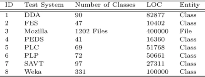
We have used 8 test systems that are devel-oped using C, C++, and Java languages to conduct the experiments. The test systems have been used in previous research (Siddique and Maqbool, 2012), (Muhammadet al., 2012), (Naseemet al., 2013). All of these test systems vary in their source code sizes and application domains. Table 29 presents the de-tails of the test software systems.

(13)

Table 29 Details of the Test Software Systems

ID Test System Number of Classes LOC Entity

1 DDA 90 82877 Class

2 FES 47 10402 Class

3 Mozilla 1202 Files 400000 File

4 PEDS 41 16360 Class

5 PLC 69 51768 Class

6 PLP 72 50661 Class

7 SAVT 97 27311 Class

8 Weka 331 100000 Class

We used two open source and six proprietary test software systems. The open source test software systems are: 1) Mozilla, an open source web browser and developed in C and C++ programming lan-guages. For experiments, we used Mozilla2 _version

1.3 released in March 2003. This test system is taken from Siddique and Maqbool (2012); 2) Weka, an-other open source software system developed in Java programming language, is a well-known data mining software system used for data pre-processing, clus-tering, regression, classification, association rules, and visualization. We use Weka3 _{version 3.4, taken}

from Siddique and Maqbool (2012), for experimental purposes.

The proprietary test software systems used for experiments are developed in Visual C++ program-ming language. They are: 1) DDA, software to de-sign the document composition and layout; 2) FES, a fact extractor software system to extract the facts of software systems; 3) PEDS, a power dispatch prob-lem solver using conventional and evolutionary com-puting techniques; 4) PLC, a printer language con-verter software system used to convert the intermedi-ate data structure to a well-known printer language; 5) PLP, a parser software system, which is used to parse a well-known printer language; 6) SAVT, a sta-tistical and analysis visualization tool. These soft-ware systems are proprietary and are currently op-erational. We obtained the extracted feature matrix from Muhammadet al.(2012).

4.2 Entities and Features

Mozilla’s data set is taken from Siddique and Maqbool (2012), who considered files as entities be-cause a .c or .cpp file contains both functions with and without classes. Hence, in this study, files are considered entities for Mozilla, and file calling is used

2_{ftp://ftp.mozilla.org/pub/mozilla.org/mozilla/releases/}

mozilla1.3/src/

3_{http://perun.pmf.uns.ac.rs/radovanovic/dmsem/cd/}

install/Weka/doc/html/Weka%203.4.5.htm

as a feature. The total number of file calling fea-ture is 258. For Weka test system, which is purely developed Java, we consider classes to be entities (Siddique and Maqbool, 2012). Since classes are considered to be the basic building blocks of object oriented languages. Siddique and Maqbool (2012) selected functions invoked, user-defined types and global variables as features for classes.

For the proprietary software systems, Muham-mad et al. (2012) considered classes to be entities. We select ten indirect features for these entities (shown in Table 30), since indirect features give better results as compared to direct features (Muhammad et al., 2012). We consider various types of test software systems that are developed in different programming languages, with different types of entities and features because we want to see whether our new proposed similarity measures are applicable to these different artifacts to make good clusters for software modularization.

Table 30 Indirect Features of the Classes in Propri-etary Test Systems That were Used for Experiments

Feature Type DDA FES PEDS PLC PLP SAVT Same Inheritance Hierarchy 98 166 70 26 64 986 Same Class Containment 58 56 12 58 144 1032 Same Class in Methods 476 384 76 162 672 1900 Same Generic Class 59 91 6 465 98 49

Same Generic Parameter 0 4 0 0 0 0

Same File 136 42 36 1812 826 264

Same Folder 2456 0 0 0 0 0

Same Macro Access 0 0 12 0 2 0

Same Global Access 918 0 0 0 268 0

Total Features 4201 743 212 2523 2074 4231

4.3 Clustering Strategies

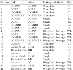
In this study, we have considered existing simi-larity measures and linkage methods that have pro-duced better results for software modularization (Muhammadet al., 2012) (Davey and Burd, 2000). In order to conduct the experiments, we categorize clustering actors into diﬀerent clustering stratagems shown in Table 31. These stratagems are composed of three existing similarity measures and four new similarity measures, using three well-known basic linkage methods. The details of these stratagems are given in Table 31.

(14)

Table 31 Clustering Stratagems

Sr. No. SM Abbr Linkage Method Abbr

1 JCJNM JCJNM Complete CL 2 JCRR JCRR Complete CL 3 JNMRR JNMRR Complete CL 4 JCJNMRR JCJNMRR Complete CL 5 JCJNM JCJNM Single SL 6 JCRR JCRR Single SL 7 JNMRR JNMRR Single SL 8 JCJNMRR JCJNMRR Single SL 9 JCJNM JCJNM Weighted Average WL 10 JCRR JCRR Weighted Average WL 11 JNMRR JNMRR Weighted Average WL 12 JCJNMRR JCJNMRR Weighted Average WL 13 Jaccard JC Complete CL 14 JaccardNM JNM Complete CL 15 Russell&Rao RR Complete CL 16 Jaccard JC Single SL 17 JaccardNM JNM Single SL 18 Russell&Rao RR Single SL

19 Jaccard JC Weighted Average WL

20 JaccardNM JNM Weighted Average WL 21 Russell&Rao RR Weighted Average WL

4.4 Assessment Criteria

To assess the output of the stratagems given in Subsection 4.3, we considered external as well as internal assessment. External assessment is the ap-proach in which expert decomposition is required to evaluate the automated results, also known as au-thoritativeness. As AHC produces results at each iteration, the following question arises: which iter-ation’s result should be evaluated? To answer the question, researchers used external criterion to eval-uate results of each iteration, and then presented the maximum or average value of the criterion (Wen and Tzerpos, 2004), (Muhammadet al., 2012), (Maqbool and Babri, 2007). We report the results by select-ing the maximum MoJoFM value out of all values obtained from each iteration. To show the strengths and weakness of the proposed and existing measures, we also evaluate the experimental results using inter-nal assessment criteria, that is, arbitrary decisions (Naseemet al., 2013) and the number of clusters pro-duced during clustering (Maqbool and Babri, 2007).

4.5 Expert Decomposition

Since we evaluated our results externally (us-ing the MoJoFM), it was important to have reliable expert decompositions with which to compare our clustering results. For the proprietary software sys-tems, expert decompositions were developed by per-sonnel having design and development experience in the software industry. They had 6 to 7 years of

ex-perience in developing software systems using C++. Some of the experts were the original developers of the software systems. We provided the source code and class listing to all the experts and asked them to develop a decomposition of the given system. The ex-perts were not provided with any details about clus-tering algorithms, and what relationships between entities were utilized during clustering. A summary of relevant statistics of the experts are presented in Table 32.

Table 32 Personnel Statistics

Personnel System Experience

in Years

Actual designer DDA 7 Experienced in C++ FES 6 Actual designer PEDS 7

Maintainer PLC 7

Actual designer PLP 6 Experienced in C++ SAVT 7

The process of preparing the expert decompo-sition is described in detail in (Muhammad et al., 2012) and (Naseem et al., 2013). These expert de-compositions have been previously used in diﬀerent studies (Naseem et al., 2013), (Muhammad et al., 2012).

For Mozilla, we used the expert decomposition used in (Siddique and Maqbool, 2012). (Siddique and Maqbool, 2012) have taken this decomposition from Xia and Tzerpos (2005). For Weka, we used the expert decomposition given in (Patel et al., 2009). This expert decomposition was provided by the orig-inal designers of the Weka software system. The expert decompositions for these systems have been used for modularization experiments earlier in (Sid-dique and Maqbool, 2012), (Patelet al., 2009), (An-dreopoulos and Tzerpos, 2005) and (Hussainet al., 2015).

5 Assessment of the new similarity

measure

In this section, we present the experimental re-sults using arbitrary decisions, number of clusters, and authoritativeness using MoJoFM measure.

(15)

5.1 Arbitrary Decision

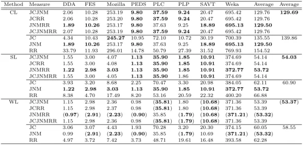
The overall results for all similarity measures are reported in Table 33. This table lists the av-erage number of arbitrary decisions that are made by the AHC using diﬀerent similarity measures in each iteration. The first column in Table 33 shows the methods, that is, CL, SL, and WL. Similarity measures are shown in the second column, while the arbitrary decision values for all test systems are given in the next eight columns. The second last column presents the average values for each similarity mea-sure, and the last column shows the average values for new and existing measures. The bold face values enclosed in parentheses indicate best values, while only bold face values represent the better values for a certain system/method.

As can be seen from Table 33, our proposed sim-ilarity measures have reduced the arbitrary decisions for each method. It is very interesting that JCJNM, JCRR and JCJNMRR measures in most cases pro-duce the same number of arbitrary decisions and also less than the existing JC and RR measures. JNMRR and JNM measures produce the same results except in two cases, where the diﬀerence is minor. Same results may be due to the fact that both similarity measures (JNM and RR) have the ability to count all features, that is,a, b, c,andd. Therefore, adding RR may have no additional eﬀect on the similarity values of JNM to reduce arbitrary decisions.

Though our proposed measures produce a less number of arbitrary decisions, the existing JNM

measure and our new JNMRR measure have the low-est number of arbitrary decisions. It is interlow-esting to note that for the SL method, the JNMRR and JNM measures produce a less number of arbitrary deci-sions for all the test systems as compared to other methods.

It can be easily observed from the second last column of Table 33 that, as was expected, our pro-posed similarity measures produced a less number of arbitrary decisions on average, as compared to exist-ing similarity measures (see the last column of Table 33).

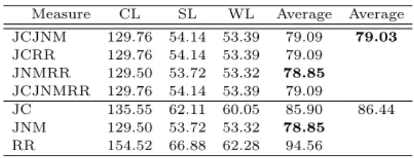
To ease the analysis, we select the average val-ues from the second last column of Table 33, and summarize them in the Table 34. Table 34 shows the average values of each similarity measure for linkage methods. It can be seen from second last column of Table 34 that for all methods on average, JNMRR and JNM produced a less number of arbitrary de-cisions. Meanwhile, last columns show the average values for all methods of our new and existing sim-ilarity measures separately in two rows. As can be seen, our new similarity measures on average pro-duced 79.03 arbitrary decisions during the clustering process which are less than arbitrary decisions pro-duced by existing similarity measures (86.44).

For further analysis, box-plots are used in Fig-ure 3 to illustrate the arbitrary decisions made dur-ing the clusterdur-ing process by AHC usdur-ing diﬀerent similarity measures. A box-plot shows the variation in the values of arbitrary decisions by indicating

Table 33 Experimental Results using Arbitrary Decisions for all Similarity Measures

Method Measure DDA FES Mozilla PEDS PLC PLP SAVT Weka Average Average CL JCJNM 2.06 10.28 253.19 9.80 37.59 9.24 20.47 695.42 129.76 129.69 JCRR 2.06 10.28 253.20 9.80 37.59 9.24 20.47 695.42 129.76 JNMRR 1.89 10.26 253.17 9.80 37.63 9.25 18.89 695.13 129.50 JCJNMRR 2.07 10.28 253.19 9.80 37.59 9.24 20.47 695.42 129.76 JC 4.34 10.43 245.27 10.95 72.10 10.72 30.19 700.39 135.55 139.86 JNM 1.89 10.26 253.17 9.80 37.63 9.25 18.89 695.13 129.50 RR 33.79 11.93 296.01 14.78 50.79 27.39 31.52 769.93 154.52 SL JCJNM 1.55 3.00 4.07 1.13 35.90 1.85 10.91 374.69 54.14 54.03 JCRR 1.55 3.00 4.08 1.13 35.90 1.85 10.91 374.69 54.14 JNMRR 1.22 2.98 3.03 1.13 35.90 1.85 10.91 372.77 53.72 JCJNMRR 1.55 3.00 4.05 1.13 35.90 1.86 10.91 374.69 54.14 JC 3.93 3.20 8.68 2.25 70.47 3.30 20.98 384.05 62.11 60.90 JNM 1.22 2.98 3.03 1.13 35.90 1.85 10.91 372.77 53.72 RR 8.38 4.70 17.49 8.20 53.16 20.59 22.32 400.20 66.88 WL JCJNM 1.15 2.98 2.36 0.98 (35.81) 1.80 (10.68) 371.36 53.39 (53.37) JCRR 1.15 2.98 2.37 0.98 (35.81) 1.80 (10.68) 371.36 53.39 JNMRR (0.97) (2.91) (2.23) (0.90) 35.85 (1.79) (10.68) (371.21) (53.32) JCJNMRR 1.15 2.98 2.36 0.98 (35.81) (1.79) (10.68) 371.36 53.39 JC 3.06 3.07 4.43 1.93 70.28 3.20 20.30 374.15 60.05 58.55 JNM 0.99 (2.91) (2.23) (0.90) 35.85 (1.79) 10.69 (371.21) (53.32) RR 4.97 3.72 7.42 3.73 48.71 19.61 16.48 393.58 62.28

unedited

(16)

Fig. 3 Arbitrary decisions made during the clustering process by all binary similarity measures using CL and SL methods for diﬀerent test software systems.

(17)

Table 34 Average Number of Arbitrary Decisions for all Similarity Measures

Measure CL SL WL Average Average JCJNM 129.76 54.14 53.39 79.09 79.03 JCRR 129.76 54.14 53.39 79.09 JNMRR 129.50 53.72 53.32 78.85 JCJNMRR 129.76 54.14 53.39 79.09 JC 135.55 62.11 60.05 85.90 86.44 JNM 129.50 53.72 53.32 78.85 RR 154.52 66.88 62.28 94.56

the quartiles and also highlights the outliers for each measure. For clarity, points are presented alongside a box-plot, which represent the number of iterations in which that many arbitrary decisions made (i.e., the number of times that value of arbitrary deci-sions arises during clustering). Thus, the density of the points shows which arbitrary decision values are mostly observed during the clustering process.

As shown in Figure 3, JC and RR produce a larger number of arbitrary decisions as compared to JCJNM, JCRR, JNMRR, JCJNMRR and JNM in general. This is apparent from the height of the box, which indicates higher dispersion. Although in some cases the height of the box is lower for JC and RR (e.g., for FES using SL), there is a higher average in Table 33 for these measures. This indicates that arbitrary decisions are being made in a large number of iterations.

We also list some important statistics for our new and existing measures. Table 35 presents, for the arbitrary decisions, the minimum value (Min), maximum value (Max), mean, standard deviation (Std), Mode, and Percentage of the count of occur-rence of mode value. The Min value for new measures is 78.85, which is equal to the Min value of existing measures. However, the Max value for new mea-sures (79.09) is smaller than the existing meamea-sures. It indicates that new measures create the maximum, which is very near to the minimum value created by both the existing and new measures. It can be seen that the Std for our new similarity measures is 0.11, which is much less than the Std value for existing similarity measures. It clearly indicates that our new similarity measures produce very compact results as compared to existing similarity measures. It can also be observed that 75% of the results produced by our proposed measures are the same, while the existing measures created varied results and hence found no mode.

Table 35 Statistics of Arbitrary Decisions

Measure Type Min Max Mean Std Mode Percentage New 78.85 79.09 79.03 0.11 79.09 75% Existing 78.85 94.56 86.44 6.42 N/A 0%

5.2 Number of Clusters

The number of clusters during the clustering process shows how compact the produced clusters are. A large number of clusters created during the clustering process indicates that created ters are highly compact, while a low number of clus-ters presents that created clusclus-ters are non-cohesive (Wang et al., 2010) (Maqbool and Babri, 2007). Hence, a high number of clusters indicates the use-fulness of the AHC approach.

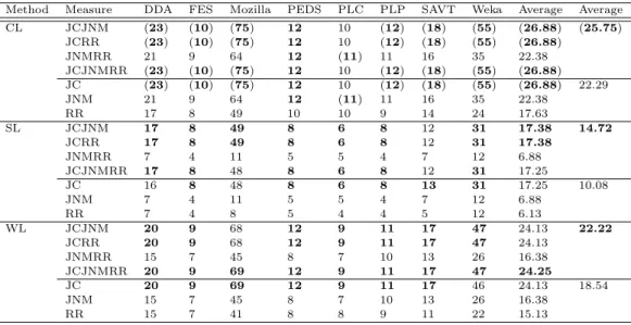
Table 36 shows the maximum number of non-singleton clusters, created by AHC during all iter-ations. The values enclosed in parentheses indicate best values, while only bold face values represent the better values for a system/method. As can be seen from Table 36, the number of clusters created by AHC using our new similarity measures is higher than that created by existing similarity measures. It can be seen that for all test software systems, JCJNM, JCRR and JC measures created a large number of clusters using the CL, SL, and WL meth-ods except for four cases, that is, CL applied on PLC, SL applied on DDA and Mozilla, and WL ap-plied on Mozilla and Weka. For the SL method, JCJNM, JCRR, and JCJNMRR measures produced a large number of clusters for all test system except one (SAVT). It is interesting to note that once again, JNMRR and JNM measures result in the same num-ber of clusters for all test software systems and link-age methods. It can also be seen that for Mozilla and Weka software systems, our new measures substan-tially increased the number of clusters similar to the JC measure. It is very interesting to note that the new measures integrating the JC similarity measure have achieved equally a large number of clusters as the JC measure. This is because our new measures (JCJNM, JCRR, and JCJNMRR) integrate the JC measure, which results in a large number of clus-ters. The JNMRR does not integrate the JC mea-sure; therefore, results are the same as those of the JNM measure.

As can be seen from the second last column of Table 36, on average for the CL method, the JCJNM, JCRR, JCJNMRR, and JC produce better results,

(18)

that is, they create a large numbers of clusters. The JCJNM and JCRR measures with the SL method and the JCJNMRR measure with the WL method result in a large number of clusters. It can be seen from the last column of Table 36 that, for each link-age method our new similarity measures outperform the existing one.

To summarize the results, we listed the values given in the second last column of Table 37 in Table 36. Table 37 presents the number of cluster values of similarity measures for linkage methods. This ta-ble clearly indicates how well a measure performs as compared to other contesting measures. This table also shows the average of each type, which indicates the average of all new measures and all existing sures separately. It can be seen that the new mea-sures outperform the existing ones by creating a large number of clusters.

Table 37 Average Number of Clusters Produced dur-ing clusterdur-ing for All Similarity Measures

Measure CL SL WL Average Average JCJNM 26.88 17.38 24.13 22.79 20.90 JCRR 26.88 17.38 24.13 22.79 JNMRR 22.38 6.88 16.38 15.21 JCJNMRR 26.88 17.25 24.25 22.79 JC 26.88 17.25 24.13 22.75 16.97 JCNM 22.38 6.88 16.38 15.21 RR 17.63 6.13 15.13 12.96

For further analysis, a violin plot is shown in Figure 4, which shows the number of clusters created during the clustering process by diﬀerent similarity

measures using CL and SL on various test software systems4_{. The clustering process starts by forming}

very small-sized clusters (size 2). Increase in the height of violin graph means that a large number of clusters are created during the clustering process. The width of the violin shows the values distribution over the observed number of clusters. It can be easily observed that our new similarity measures and JC (in most of the cases) result in a large number of clusters. It can also be seen that JNM, RR, and JNMRR measures produce a relatively fewer number of clusters during the clustering process. This is especially true for the SL measure, where the number of clusters during clustering is much lower for these measures.

To support the claim that our proposed mea-sures perform better, Table 38 shows the statistics of Table 37. All the statistical data (Min, Max, Mean, Std, Mode and Percentage) are derived from the sec-ond last column of Table 37. The Min value for new measures is 15.21, which is greater than the Min value of existing measures (12.96). The Max value for the new measures is slightly greater than the ex-isting measures. It can be seen that the Std value for our proposed measures (3.28) is less than the existing measures, which indicates that our new measure’s re-sults are close to the mean value and are also close to each other. This table also shows the Mode and

4_{Due to the limited space only the results of CL and SL}

methods employed on DDA, FES, Mozilla, PEDS and PLC test software systems are presented

Table 36 Experimental Results using Number of Clusters Produced during Clustering for All Similarity Measures

Method Measure DDA FES Mozilla PEDS PLC PLP SAVT Weka Average Average CL JCJNM (23) (10) (75) 12 10 (12) (18) (55) (26.88) (25.75) JCRR (23) (10) (75) 12 10 (12) (18) (55) (26.88) JNMRR 21 9 64 12 (11) 11 16 35 22.38 JCJNMRR (23) (10) (75) 12 10 (12) (18) (55) (26.88) JC (23) (10) (75) 12 10 (12) (18) (55) (26.88) 22.29 JNM 21 9 64 12 (11) 11 16 35 22.38 RR 17 8 49 10 10 9 14 24 17.63 SL JCJNM 17 8 49 8 6 8 12 31 17.38 14.72 JCRR 17 8 49 8 6 8 12 31 17.38 JNMRR 7 4 11 5 5 4 7 12 6.88 JCJNMRR 17 8 48 8 6 8 12 31 17.25 JC 16 8 48 8 6 8 13 31 17.25 10.08 JNM 7 4 11 5 5 4 7 12 6.88 RR 7 4 8 5 4 4 5 12 6.13 WL JCJNM 20 9 68 12 9 11 17 47 24.13 22.22 JCRR 20 9 68 12 9 11 17 47 24.13 JNMRR 15 7 45 8 7 10 13 26 16.38 JCJNMRR 20 9 69 12 9 11 17 47 24.25 JC 20 9 69 12 9 11 17 46 24.13 18.54 JNM 15 7 45 8 7 10 13 26 16.38 RR 15 7 41 8 8 9 11 22 15.13

unedited

(19)

Fig. 4 Number of clusters created by all binary similarity measures during the clustering process using CL and SL methods for diﬀerent test software systems.

(20)

Percentage of mode value’s occurrence. The mode for new measures is 22.79 which occurs three times in the second column of Table 38. The percentage value 75 means that 75% values are the same for the JCJNM, JCRR and JCJNMRR similarity measures. Table 38 Statistics of Number of Clusters Based on Table 37

Measure Type Min Max Mean Std Mode Percentage New 15.21 22.79 20.90 3.28 22.79 75% Existing 12.96 22.75 16.97 4.19 #N/A 0%

5.3 Authoritativeness

The automated result is required to approxi-mate the decomposition prepared by a human ex-pert (an authority). For this purpose we use Mo-JoFM to compare the automated results with the expert decompositions. The MoJoFM values for the series of experiments are given in Table 39. This table shows the maximum MoJoFM values selected during the iterations of the clustering process for all similarity measures and test software systems. The bold face values indicate the better values for a test system/method. The values enclosed in parenthe-ses indicate best values in the Table 39. The aver-age values for each similarity measure is shown in the second last column of Table 39, while the last column presents the average for new measures and existing measures and are based on the average val-ues given in the second last column. As can be seen from Table 39, in most of the cases our new mea-sures outperform the existing ones. This is because in previous Subsections 5.1 and 5.2, we have shown that our new similarity measures result in a smaller number of arbitrary decisions and a large number of clusters. Thus reducing arbitrary decisions and in-creasing the number of clusters improve the author-itativeness of the automated results (Naseemet al., 2013) (Maqbool and Babri, 2007).

It can be easily analyzed that our new measures produce better results than the existing measures ex-cept for one test software system, that is, the PLC software system where results of the JNM measure using the CL method, is better. As can be seen from Table 39, for the DDA software system the JNMRR measure using the CL method results in the high-est MoJoFM value. For the FES software system, the JCJNM, JCRR, and JCJNMRR measures using the CL method produce better results as compared

to all other stratagems. For the Mozilla test system, the JNMRR similarity measure using the CL method gives the highest MoJoFM value. For the PEDS soft-ware system, our new and existing measures perform equally well. PLC is the only test systems for which the existing JNM measure using the CL method re-sults in the highest MoJoFM value. For the PLP software system, all the existing measures using the CL method give the highest value, while for SAVT test software system JNMRR measure using the CL method and JCJNM and JCRR measures using the WL method result in the highest MoJoFM values (67.03%). Lastly, for the Weka software system, the JCJNM and JCRR measures using the WL method produce the highest MoJoFM values as compared to other measures using the CL and SL methods.

As can be seen from the second last column in Table 39, on average our new measures outperform the existing measures. The last column of Table 39 shows the average values of the new and existing sim-ilarity measures, respectively. As can be seen, our new measures outperform all existing measures us-ing all linkage methods on all test software systems. Meanwhile, the CL method results in the highest MoJoFM value. Hence we can infer that the CL method produces better results as compared to the SL method, while the WL method falls in between these two.

To show results more precisely, Table 40 lists average values from the second last column of Table 39 for each similarity measure. It can be seen from Table 40, that for the CL method, the JNMRR mea-sure results in better MoJoFM values as compared to other similarity measures. For the SL method, JCJNMRR measure yields better results, while for the WL method, the JCJNM and JCRR produce better results. As can be seen from the second last column of Table 40, on average, the JCJNMRR pro-duces better result as compared to all other similarity measures. This table also provides good evidence to say that our new measures produce better results as compared to existing measures for all linkage meth-ods.

Table 41 lists diﬀerent statistics based on values in the second last column of Table 40. It can be seen that Min, Max, and Mean values for proposed new measures are higher than the existing measures. It indicates that in all cases, our new measures produce better results. These values indicate the superiority

(21)

Table 39 MoJoFM Results for all Similarity Measures

Method Measure DDA FES Mozilla PEDS PLC PLP SAVT Weka Average Average CL JCJNM 56.25 45.00 63.89 57.14 61.54 (65.67) 65.93 30.45 55.73 (55.94) JCRR 56.25 45.00 63.89 57.14 61.54 65.67 65.93 30.45 55.73 JNMRR (60.00) 45.00 64.68 57.14 61.54 65.67 (67.03) 30.13 (56.40) JCJNMRR 57.50 45.00 63.89 57.14 61.54 65.67 65.93 30.45 55.89 JC 56.25 43.00 63.00 57.14 61.00 51.00 54.00 30.45 51.98 52.45 JNM 56.25 43.00 64.00 57.14 (65.00) 60.00 54.00 30.13 53.69 RR 53.75 38.00 62.00 57.14 64.00 55.00 58.00 25.64 51.69 SL JCJNM 53.75 (47.50) 46.03 57.14 63.08 59.70 58.24 22.12 50.95 47.97 JCRR 53.75 (47.50) 46.03 57.14 63.08 59.70 58.24 22.12 50.95 JNMRR 25.00 32.50 35.71 54.29 60.00 38.81 47.25 17.31 38.86 JCJNMRR 53.75 (47.50) 46.03 57.14 64.62 59.70 58.24 22.12 51.14 JC 53.75 35.00 46.00 54.29 55.00 28.00 32.00 23.08 40.89 36.16 JNM 25.00 43.00 36.00 54.29 42.00 28.00 32.00 17.31 34.70 RR 23.75 33.00 36.00 51.43 42.00 28.00 32.00 16.99 32.90 WL JCJNM 56.25 42.50 61.11 57.14 63.08 59.70 (67.03) (32.05) 54.86 53.95 JCRR 56.25 42.50 61.11 57.14 63.08 59.70 (67.03) (32.05) 54.86 JNMRR 50.00 40.00 56.35 54.29 63.08 58.21 63.74 24.68 51.29 JCJNMRR 56.25 42.50 62.30 57.14 63.08 59.70 (67.03) 30.45 54.81 JC 56.25 38.00 61.00 57.14 56.00 46.00 48.00 31.09 49.19 49.40 JNM 50.00 35.00 61.00 54.29 55.00 55.00 53.00 24.68 48.50 RR 52.50 45.00 62.00 54.29 61.00 55.00 51.00 23.40 50.52

of our new measures over existing measures. Stan-dard deviation (Std) values for both type of measures indicates that each type has one value that is out of the range. Meanwhile, the JCJNM and JCRR mea-sures result in exactly the same values, which can be seen in Table 40 and Table 41 (column Mode). The percentage value 50 means that 50% values are the same, that is, for the JCJNM and JCRR similarity measures.

Table 40 Average MoJoFM Results for all Similarity Measures

Measure CL SL WL Average Average JCJNM 55.73 50.95 54.86 53.85 52.62 JCRR 55.73 50.95 54.86 53.85 JNMRR 56.40 38.86 51.29 48.85 JCJNMRR 55.89 51.14 54.81 53.94 JC 51.98 40.89 49.19 47.35 46.01 JNM 53.69 34.70 48.50 45.63 RR 51.69 32.90 50.52 45.04

Table 41 Statistics for New and Existing Measure based on Table 40

Measure Type Min Max Mean Std Mode Percentage New 48.85 53.94 52.62 2.18 53.85 50% Existing 45.04 47.35 46.01 0.98 #N/A 0%

5.3.1 Significance of the Authoritativeness

In order to show the significance of the authori-tativeness’ results, the t-test is conducted to show if there is significant diﬀerence between the MoJoFM values of new measures and the existing measures. In this case, null hypothesisHois as follows: “There

is no diﬀerence between the MoJoFM values of new measures and the existing measures”.

Table 42 The T-test Values between the MoJoFM Results of the New and Existing Measures using CL and SL Method

New Measures Existing Measures CL SL JCJNM JCJNM 1.901.30 2.414.10 RR 2.79 5.10 JCRR JCJNM 1.901.30 2.414.10 RR 2.79 5.10 JNMRR JCJNM 2.241.64 -0.451.31 RR 3.19 2.39 JCJNMRR JC 2.01 2.46 JNM 1.42 4.11 RR 2.93 5.12

T-test (withdf = 7) is conducted between the new and existing measures using CL and SL meth-ods. The t-test results are given in Table 42. This table clearly indicates that ift>2.365, then the new measures have significantly performed better at 95% confidence level; at this level of confidence, all new measures are significantly better than RR using the CL method, and JCJNM, JCRR, and JCJNMRR are better than all existing measures using SL. Moreover, JNMRR is significantly better than RR using the SL method. At 90% confidence level (t > 1.895), all new measures are significantly better than JC using the CL method. At 80% confidence level (t>1.415), JNMRR and JCJNMRR are significantly better than JNM using the CL method. Finally, the JCJNM and JCRR are significantly better than JNM using

(22)

the CL method at 70% confidence level (t >1.12). Thus, the new measures produced significantly bet-ter results at diﬀerent confidence levels; hence, the null hypothesisHois rejected.

5.4 Summary of Results

Considering the overall performance of the similarity measures, our new similarity measures (JCJNM, JCRR, JNMRR, and JCJNMRR) outper-form the existing similarity measures (JC, JNM and RR) using the CL, SL and WL methods with respect to authoritativeness, number of clusters and arbi-trary decisions. It can be noticed that for most of the cases the JCJNM, JCRR, and JCJNMRR mea-sures yield better results. However, on average the JNMRR using the CL method results in the high-est authoritativeness value as shown in Table 39. The JCJNM and JCRR measures used with the WL method achieve the second position, and the JCJN-MRR measure using the SL method is on the third position. On average, the JCJNMRR measure gives better authoritativeness for all methods as compared to all other measures, which can be seen in Table 40. Experimental results in terms of the number of clusters reveal that for all test software systems, the JCJNM, JCRR, JCJNMRR and JC measures using the CL method yield better results, as can be seen in Table 36. However, for all methods, the JCJNM measure performs better as shown in Table 37.

As can be seen from Table 33, the JNMRR mea-sure using the WL method creates the lowest arbi-trary decisions for all test software systems, as com-pared to other stratagems. For all methods, the JN-MRR and JNM measures produce a less number of arbitrary decisions, as shown in Table 34.

As compared to the SL and WL methods, the CL method yield better results for authoritativeness for all the test software systems, as shown in Table 39. The WL method results in a less number of arbitrary decisions, as presented in Table 33. The CL method creates a large number of clusters during clustering as compared to the WL and SL methods, which can be seen in Table 36.

5.5 Threats to Validity

The selection of test systems may pose a threat to a study, since the test system characteristics may influence the results. To reduce this threat, we

se-lected open and closed source software systems of dif-ferent sizes (numbers of source lines) having diﬀerent application domains. We used 8 test systems devel-oped in well-known programming languages, that is, C, C++, and Java. However, more experiments may be conducted on large-size software systems devel-oped in other programming languages.

In order to evaluate the results, we used Mo-JoFM as the external assessment criterion, and used the number of clusters and the number of arbitrary decisions as the internal assessment criteria. As Mo-JoFM requires an expert decomposition prepared by a human, a threat may exist during the preparation of expert decomposition due to human biases. How-ever, we have tried to reduce this threat by selecting experienced software personnel as experts, who were also involved in the development of the proprietary software systems. For Mozilla, expert decomposi-tion is prepared by the authors of (Godfrey and Lee, 2000) and then updated for the Mozilla 1.3 by the authors of (Xia and Tzerpos, 2005) and for Weka we used the decomposition prepared by the actual de-signers of the systems (Patelet al., 2009). Moreover, we selected software systems that have been used in previous studies, with their expert decompositions (Siddique and Maqbool, 2012) (Muhammad et al., 2012) (Patel et al., 2009) (Andreopoulos and Tzer-pos, 2005) (Hussain et al., 2015). Since our main goal was to integrate the strengths of existing mea-sures, our choices of internal assessment criteria are based on that goal. We are aware that there exist a number of other internal assessment criteria, for ex-ample, coupling and cohesion that can also be used to investigate the results.

6 Conclusions

This paper presents the improved binary simi-larity measures, namely, JCJNM, JCRR, JNMRR, and JCJNMRR for clustering software systems for modularization. These measures integrate the strengths of the following existing binary similar-ity measures: Jaccard (JC), JaccardNM (JNM), and Russell&Rao (RR). An example of the existing and new similarity measures is presented to show how our new measures integrate strengths of the existing similarity measures. We present empirical results to compare the results of the existing and new simi-larity measures and show the strengths of our new