Multiscale models for structure and dynamics of confined fluids

(1)

c

(2)

MULTISCALE MODELS FOR STRUCTURE AND DYNAMICS OF CONFINED

FLUIDS

BY

TARUN SANGHI

DISSERTATION

Submitted in partial fulfillment of the requirements

for the degree of Doctor of Philosophy in Mechanical Engineering

in the Graduate College of the

University of Illinois at Urbana-Champaign, 2016

Urbana, Illinois

Doctoral Committee:

Professor Narayana R. Aluru, Chair and Director of Research

Professor Klaus J. Schulten

Professor Kenneth S. Schweizer

(3)

Abstract

In this dissertation, using systematic coarse-graining, we develop multiscale models to study structural and dynamical properties of confined fluids. With the advent of nanofluidics and nanobiotechnology, fluids confined inside nanometer scale geometries have become a subject of both fundamental investigation and applied research. An understanding of the structural and dynamical properties of fluids at nanoscale is essential for designing novel engineering applications such as nanofiltration, carbon-dioxide sequestration, single-file transport, nanomedicine and many others. Our structural model is based on an empirical potential based quasi-continuum theory (EQT). EQT is a multiscale theory that seamlessly integrates the interatomic potentials describing various atomic interactions into a continuum framework to obtain the equilibrium den-sity and potential profiles of confined fluids in a self-consistent manner. The denden-sity and potential profiles obtained from it are comparable in accuracy with those obtained from particle-based methods such as molec-ular dynamics (MD) simulations. Also, being a continuum approach, EQT is very simple to implement and is computationally several orders of magnitude faster than MD simulations. The central task in EQT is the development of quasi-continuum potential models that accurately describe the wall-fluid and fluid-fluid in-teractions in confined fluids. Using systematic coarse-graining, we discuss the development of coarse-grained single-site (CGSS) pair-potentials and quasi-continuum potential models for poly-atomic fluids. Proposed potential models systematically incorporate the effect of size, geometric shape and orientation of poly-atomic fluids to predict the correct microstructure in confined environments. We take carbon-dioxide as an exam-ple fluid and demonstrate the applicability of the potentials models in EQT as well as coarse-grained MD (CG-MD) simulations to predict the center-of-mass (COM) density and potential profiles of carbon-dioxide inside slit-shape graphite nanochannels at several high and low pressure confinements. The results obtained from EQT and CG-MD simulations are found in good agreement with those obtained from all-atom MD (AA-MD) simulations.

To develop dynamical models, one fundamental question is to understand the role of thermal noise in nanofluidic dynamics and transport. We discuss a combined memory function equation (MFE) and generalized Langevin equation (GLE) based approach (referred to as MFE/GLE formulation) to characterize

(4)

thermal noise in molecular fluids. Using MFE/GLE formulation in conjunction with MD simulation, we extract and analyze the statistical properties of thermal noise in confined fluids. We find that the thermal noise correlation time of the confined fluid does not vary significantly across the confinement and is quite similar to that of the corresponding reference bulk state fluid. We show that it is the cross-correlation of the mean force with the molecular velocity that gives rise to the spatial anisotropy in the velocity-autocorrelation function of the confined fluids. Further, we demonstrate that using the noise characteristics of reference bulk state fluid, and the structural information obtained from EQT, GLE can be used to simulate the single-particle dynamical properties of confined fluids. As an application, we use the GLE formulation to compute the interfacial friction coefficient at solid-liquid interface. Interfacial friction coefficient is an important macroscopic modeling parameter that provides the atomistic to continuum bridge by incorporating the effect of the wall-lattice structure and the nature of wall-fluid interactions on the fluid transport. The attractive feature of the GLE approach is that all the inputs to the GLE are obtained from EQT and simulation data of the reference bulk state fluid, thereby eliminating the need to perform computationally expensive equilibrium molecular dynamics (EMD) simulation of the confined system to estimate the interfacial friction. We also use the GLE formulation to understand the memory effects in the dynamics and transport of nanoparticles such as fullerenes immersed in host fluid environment. Finally, we discuss a GLE based approach to simulate the dynamics of interacting-particles.

(5)

(6)

Acknowledgments

This thesis would not have been possible without the support and encouragement of a lot of people. First and foremost, I wish to express my gratitude to my Ph.D. advisor, Prof. Narayana R. Aluru, for his constant guidance and encouragement, throughout the course of my doctoral research. I would also like to thank Prof. Klaus J. Schulten, Prof. Kenneth S. Schweizer and Prof. Andrew L. Ferguson, for serving on my doctoral committee. I also wish to thank all former and present members of Prof. Aluru’s research group. The group has been a source of good advice, collaboration and friendship. In particular, I would like to thank Kumar Kunal, Ravi Bhadauria, Sikandar Mashayak and Joonho Lee for numerous helpful discussions. I acknowledge the Eugen and Lina Abraham Endowed Ph.D. Supplemental Fellowship (2010) and Shaller Fund travel award (2012) from the department of Mechanical Science and Engineering. I also acknowledge the use of parallel computing resources provided by the Computational Science and Engineering Program at the University of Illinois.

During my stay at Urbana-Champaign, I was fortunate to make some lifelong friends. I would like to thank all of them, especially Vikas, Nitin, Kunal, Sahu, Chandu, Sucheta, Ravi, Navin and Tanvee. Finally, I would like to thank my family for their love and constant support through all these years. It would be an understatement to say that this work would not have been possible without my family, and I dedicate this thesis to them.

(7)

List of Tables

2.1 Parameters of CGSS wall-fluid and fluid-fluid interaction potentials. . . 19

2.2 Softer repulsive core parameters . . . 24

3.1 Thermal noise correlation time,τR, and the momentum relaxation time,τv in fluidic systems. 34 3.2 Statistical moments of the thermal forceRq(t) as extracted from the MD simulation. . . 37

4.1 Friction coefficientζ0 (kJ-ps/mol/nm2) . . . 53

5.1 Scaling of memory with the mass of nanoparticle. . . 61

5.2 Scaling of memory with shape and size of nanoparticle. . . 64

5.3 Effect of memory on transport properties of nanoparticle. . . 68

(10)

List of Figures

2.1 Atomistic (a) and Continuum (b) representation of fluid confined inside a slit shape nanochan-nel. H is channel width,ρwall is wall density andρ(z) is fluid density . . . 7

2.2 Computation of the wall-fluid and fluid-fluid interaction energy in the quasi-continuum for-mulation. (Figure courtesy of Mohammad Hossein Motevaselian). . . 9 2.3 Comparison ofuAA_{f f}(r) andut_{f f}(r). σf f is the fluid atomic diameter. . . 11 2.4 Comparison of density profile from EQT (solid line) and MD simulation (open circle). σf f is

the fluid atomic diameter. . . 12 2.5 COM density of confined CO2from a bulk CGSS potential model [1](broken line) and a 3-site

AA potential model [2] (solid line). . . 13 2.6 (a) COM density profile, ρ(z), (b) Molecular orientation profile, Sθ, (c) Functional form of

uCGSSwall-CO2(r) and u

CGSS

CO2-CO2(r), and (d) Relative orientation profile of CO2 confined inside

a 2.232 nm wide graphite slit nanochannel. Inset: COM coordinate system used to define relative orientation. . . 15 2.7 Comparison of (a) CG wall-fluid PMF profile, U_wallCG_-_CO

2, (solid line) and (b) CG fluid-fluid

PMF profile,U_COCG

2-CO2, (solid line) with their respective target AA-MD PMF profiles (open

circle) for carbon dioxide confined inside a 2.232 nm wide graphite slit nanochannel at T = 323 K and P = 10.1 MPa. The reference potential value is subtracted from each PMF profile while plotting. . . 19 2.8 Comparison of the CG wall-fluid PMF,U_wallCG_-_CO

2, (left) and the CG fluid-fluid PMF,U

CG CO2-CO2,

(right) profiles obtained from CGSS potentials (solid line) with their respective target AA-MD PMF profiles (open circle) at different thermodynamic states. The reference potential value is subtracted from each PMF profile while plotting. . . 21 2.9 Comparison of the COM density and potential profiles obtained by using the quasi-continuum

potentials in EQT (solid line) with those obtained from AA-MD simulations (open circle) for supercritical carbon dioxide (T = 348 K and P = 9.05 MPa) confined insideH = 2.232 nm and

H = 1.488 nm wide graphite slit nanochannels. The reference potential value is subtracted from each PMF profile while plotting. . . 23 2.10 COM density profile of carbon dioxide confined inside different width graphite slit

nanochan-nels at a high pressure (left) and a low pressure (right) confinement state. Solid line represents the results from EQT and open circle are the AA-MD results. ρavg is reported in units of

molecules/nm3. . . 25 2.11 COM density profile of carbon dioxide confined inside different width graphite slit

nanochan-nels at two different supercritical temperature states. Solid line represents the results from EQT and open circle are the AA-MD results. ρavg is reported in units of molecules/nm3. . . 25

2.12 Comparison of the COM density profile obtained from CG-MD simulations (solid line) with those obtained from AA-MD simulations (open circle). . . 27 2.13 Comparison of the COM density profile inside H = 0.60 nm (left) and H = 0.744 nm (right)

slit nanochannels as obtained from CG-MD simulations (broken line) and EQT (solid line) with those obtained from AA-MD simulations (open circle). . . 28 3.1 Comparison of the COM v-ACF (solid line) andR-ACF (broken line) for (a) bulk CO2 and

(11)

3.2 (a) Schematic of a semi-infinite slit nanochannel, (b) Number densityρ(z), (c)-(d) Mean force profiles (Force is in kJ/mol-nm), (e)v-ACFs alongx(broken line) andz(solid line) directions, (f) Variation of Θz(t) and (g) Memory functionsKx(t) (broken line) andKz(t) (solid line) of

SPC/E water confined inside a graphite slit. . . 36 3.3 Frequency distribution of the thermal force. . . 38 3.4 (a) Number densityρ(z), (b)-(c) Mean force profiles (Force is in kJ/mol-nm), (d)v-ACFs along

x (broken line) and z (solid line) directions, (e) Variation of Θz(t), Θx(t) and (f) Memory

functionsKx(t) (broken line) andKz(t) (solid line) of SPC/E water confined inside a silicon slit-shape nanochannel . . . 39 3.5 (a) v-ACF (Inset: Enlarged view [0-1] ps) and (b) Memory function K(t) (Inset: Enlarged

view [0-0.8] ps) of SPC/E water confined inside different size CNTs. . . 41 3.6 a) Mean force profileFz, (b) Memory functionK(t), (c) MSD (Inset: Enlarged view [0-0.5] ps)

and (d) Survival probability of confined LJ argon as obtained from GLE and MD simulations. 44 4.1 Computation of interfacial coefficient in a slit-shape nanochannel. . . 47 4.2 (a) Memory function of SPC/E bulk water (blue line) at 298 K and density 33.46 molecules/nm3.

Also plotted are memory function of water in the streaming (green dash-dot line) and confined (red dashed line) direction for 4σff wide Silicon-water system. Mean wall-fluid (solid blue line) and total (red open circles) force in the streaming direction for (b) graphene-water, and (c) silicon-water interface. . . 49 4.3 Wall-fluid FACF from GLE (bold line, blue) and EMD (circles, red) for (a) graphene-water

and (b) silicon-water interfaces. (c) FVCCF from GLE and EMD for water with graphene and silicon interfaces. . . 52 5.1 Fullerene nanoparticles studied: (a) C60, (b) C100, (c) C180, (d) C240. . . 55 5.2 Comparison of (a) Momentum autocorrelation function,C(t), (b) Total force autocorrelation,

F-ACF, (c) Memory function, K(t), (Inset: Normalized K(t)), (d) Projected force autocor-relation,F+-ACF, (Inset: Comparison ofF-ACF andF+-ACF forM/m=4000) for different mass C60 immersed in water. . . 59 5.3 Comparison of (a) Momentum autocorrelation function,C(t), (b) Total force autocorrelation,

F-ACF and (c) Memory function, K(t) for different shape and size nanoparticles (M/m=40) immersed in water. . . 63 5.4 Scaling of the momentum autocorrelation function with the magnitude of the memory function

in GLE simulation. . . 66 5.5 The time dependence of the probability densityW(θ, t) for θ= 30, 60, 120 and 150 degrees.

Solid line is GLE, broken line is SLE and open circle is MD simulation result. . . 67 5.6 Schematic of transport of C60 immersed in water across a 1-D potential barrierU(X). . . 69 6.1 Particle interaction in MD and GLD simulations. . . 71 6.2 Radial distribution function (top) and pair-interaction forceF₁₂GLD (bottom) used in GLD. . 74 6.3 Comparison of (a) velocity autocorrelation function,Ci(t), (b) force-velocity cross-correlation

function, FVCCF, and (c) radial distribution function, g(r), as obtained from GLD (using single-particle memory function) and MD simulation. . . 77 6.4 Memory function obtained from single-particle MFE (Eq. (6.5)) and interacting-particle MFE

(Eq. (6.6)). . . 78 6.5 Comparison of (a) velocity autocorrelation function, Ci(t), (b) radial distribution function,

g(r), and (c) mean-square displacement (MSD), as obtained from GLD (using interacting-particle memory function) and MD simulation. . . 79 6.6 Comparison of distinct van-Hove function Gd(r, t) for (a) LJ Methane, and (b) LJ Argon,

from interacting-particle GLD and MD simulation. . . 81 6.7 Comparison of the time decay of (a) kinetic-kinetic SACF, zkk_αβ(τ), (b) potential-potential

SACF, zpp_αβ(τ), and (c) kinetic-potential SACF, zkp_αβ(τ), for LJ Methane as obtained from GLD and MD simulation. . . 84

(12)

6.8 Comparison of the time decay of (a) kinetic-kinetic SACF, zkkαβ(τ), (b) potential-potential

SACF,zpp_αβ(τ), and (c) kinetic-potential SACF,z_αβkp(τ), for LJ Argon as obtained from GLD and MD simulation. . . 85

(13)

Chapter 1

Introduction

1.1 Motivation

With the advent of nanofluidics and nanobiotechnology, fluids confined inside nanometer scale geometries have become a subject of both fundamental investigation and applied research. An understanding of the structural and dynamical properties of fluids at nanoscale is essential for designing novel engineering ap-plications such as nanofiltration [3–5], carbon-dioxide sequestration [6, 7], single-file transport [4, 8–12], nanomedicine [13] and many others. Computational analysis plays a very important role in the design and optimization of these nanofluidic devices. Also, computational analysis can provide fundamental insights into nanoscale flow physics, which could be hard to characterize in experiments. Inside nanoscale confinements, due to the strong interaction of the surface with the fluid, the fluid becomes inhomogeneous and exhibits behavior that is quite different from the corresponding bulk state [14]. Also, at such smaller scales, thermal fluctuations influence the flow characteristics [15–18] at the solid-fluid interface. Continuum or classical theories, which assume a homogeneous variation of state variables and ignore the discrete atomic structure of the fluid and the confining wall molecules, fail to predict the correct behavior at nanoscale confinement. Also, most continuum based classical theories ignore thermal fluctuations. Hence, it is imperative to develop computational models/strategies that incorporate the missing atomic-scale physics into the classical theories to study the fluid behavior in nanoscale confinements.

1.2 Survey of computational approaches for confined fluids

In the past four decades, a great deal of progress has been made towards developing both theoretical and computer simulation based tools to study confined fluids. Statistical physics based models, which explicitly include the finite-size and discrete atomic structure of the fluid and the confining wall molecules, are used to study fluid confined inside nanometer scale geometries. From a theoretical standpoint, several approaches based on the modified kinetic theory (modified Enskog theory, local average density model) [19, 20], density functional theory (DFT) [21, 22] and integral equation theory (IET) [23] are proposed that can predict the

(14)

static and dynamical properties of confined fluids. Though most of these theories have a firm statistical foundation, from an engineering viewpoint, they are very difficult to implement and computationally ex-pensive to study general nanoscale flow problems. Extension and application of these approaches beyond structureless hard-sphere and simple Lennard-Jones (LJ) type fluids is rather complicated and is still an active area of research [20, 24].

From a simulation standpoint, with the dramatic increase in computational power during the last two decades, atomistic molecular dynamics (MD) [25] has emerged as a powerful simulation tool to study confined fluids. While MD simulation can accurately predict the structural and dynamical properties, and has greatly enhanced our understanding of the behavior of confined fluids, it requires enormous computing resources that practically inhibits its usage to study systems at length and time scales of practical interest (experimental time scales). This practical limitation of MD arises from the usage of very stiff inter-atomic potentials, which are physically needed to incorporate the finite-size and excluded volume effect, but computationally limit the largest time step that can be used to perform a stable simulation. To overcome this limitation, the concept of coarse-graining is used. In coarse-graining, softer interaction potentials are constructed from the stiff atomistic potentials either by (a) averaging the molecular field over the rapidly fluctuating short time scale motions that are lesser relevant to the macroscale phenomena of interest [26], or by (b) constructing a reduced order representation of the actual system and designing effective or coarse-grained (CG) potentials that reproduce the desired macroscopic quantity of interest [27–29]. Further, CG potentials are used to develop multiscale models that attempt to combine the atomic-scale and continuum-scale methods and provide a unified framework to study fluid behavior across a broader spectrum of length and time scales. Although CG potentials allow the simulation of systems closer to experimental scales, they have some limitations. By definition, there is a loss of structural and dynamical information in coarse-graining. During coarse-graining, the structural and chemical details of the system at scales smaller than the coarse-grained scale are completely lost. Also, most CG potentials only perform well in the thermodynamic conditions of the reference atomistic system used to parameterize them and suffer from the loss of transferability [30–32]. In recent years, a lot of effort is devoted in developing systematic approaches to coarse-graining. There exist several systematic techniques such as iterative Boltzmann inversion (IBI) [33], inverse Monte Carlo (IMC) [34], potential of mean force (PMF) matching [35], relative entropy minimization [36, 37], and force-matching (FM) [27, 38] that can be used to construct CG potentials for confined fluids. These CG potentials yield an accurate description of the static properties of the underlying reference system. However, they fail to reproduce the correct dynamical properties such as diffusivity and viscosity. This discrepancy in the dynamical quantities occurs because these techniques completely ignore the instantaneous force fluctuations that the coarse-grained or eliminated degrees of freedom exert on the retained degrees of freedom. These

(15)

instantaneous force fluctuations must be explicitly incorporated into CG description to correctly reproduce the dynamical behavior. Dissipative particle dynamics (DPD) [14, 39, 40] is one such simulation method, which has been extensively used to study the dynamics of complex fluids such as colloidal suspensions, polymer melts, etc., at length and time scales far beyond the reach of MD simulations. In DPD model, CG particles interact by three forces: a softer conservative force, a dissipative force and a random force. Softer conservative force characterizes the structure and dissipative and random forces together provide the force fluctuations that the eliminated degrees of freedom exert on the retained degrees of freedom. Although DPD is very simple to implement and conserves both mass and momentum, it fails to reproduce the structural and dynamical properties of both bulk and confined fluids. This limitation of DPD stems from the fact that in high density bulk and confined fluids, the time scales of fluid motion and thermal fluctuations are not separable and the Markovian approximation on which DPD model is based, is not valid. Also, the softer conservative force used in DPD, which allows the use of a time step significantly larger than MD simulations, does not preserve the atomic structure (radial distribution function) of the fluid. Moreover, the functional form of the softer conservative force used in DPD model is an ansatz, and it is not clear how such softer conservative potentials can be developed using systematic coarse-graining. The development of a non-Markovian DPD framework, which retains all the nice features of Markovian-DPD, and reproduces both the structural and dynamical properties of confined fluid is an open problem [41].

There also exist hybrid combined atomistic-continuum approaches [42–46], in which continuum model is solved in one part of the domain while MD is solved in another part, usually around the boundary. An overlapping region is used between these two domains in which the two descriptions are forced to match each other by either constrained MD or Schwartz iteration [45, 46]. The Schwartz iteration method is used to ensure that the two descriptions are consistent in an overlapping region at the steady state. Although the idea is quite natural and promising, these methods have had limited success, especially in predicting dynamical properties, due to coupling of the time scales and complexity of the algorithms.

1.3 Research objectives

In this research work, using systematic coarse-graining, we develop multiscale models to study structural and dynamical properties of confined fluid. The first objective of this research is based on an empirical potential based quasi-continuum theory (EQT), proposed by Raghunathan, Park and Aluru [47], to predict the equilibrium structure (inhomogeneous density and potential profiles) of confined fluids. EQT is a multi-scale theory that seamlessly integrates the interatomic potentials describing various atomic interactions into a continuum framework to obtain the equilibrium density and potential profiles in a self-consistent manner.

(16)

As EQT incorporates the finite-size and excluded volume effects through interatomic potentials, the density and potential profiles obtained from it are comparable in accuracy with those obtained from particle-based methods such as MD simulations. Also, being a continuum approach, EQT is very simple to implement and is computationally several orders of magnitude faster than MD simulations. The central task in EQT is the development of CG quasi-continuum potential models that accurately describe the wall-fluid and fluid-fluid interactions in confined fluids. The original work by Raghunathan et al. [47] discussed the development and parameterization of quasi-continuum potentials for spherical LJ-type fluids using the PMF matching technique. Although these quasi-continuum potentials include the finite-size and excluded volume effects, they suffer from the usual limitations associated with coarse-graining. In these models, the fluid and the wall structure is described in terms of density and all the structural and chemical details are lost. Also, these potential models are thermodynamic state dependent. The issue of thermodynamic transferability was considered in a subsequent work by Sanghi and Aluru [48], and two thermodynamic state dependent scaling relations were obtained (normalized by LJ energy and distance parameters) to parameterize the quasi-continuum potentials for different LJ type fluids across a wide range of thermodynamic states. Such scaling relations allow one to parameterize the quasi-continuum potentials without using computationally expensive MD simulation. With the successful application of EQT to simple LJ type fluids, the first spe-cific objective of my research is to extend it to study poly-atomic fluids. We discuss the development of quasi-continuum potential models that incorporate the effect of size, geometric shape and orientation of poly-atomic fluids. The developed potentials are used in both coarse-gained MD (CG-MD) and EQT to predict the center-of-mass (COM) density and potential profiles of carbon-dioxide confined inside graphite slit nanochannels.

The second objective of my research is to utilize the structural information obtained from EQT and develop computational approaches to study the dynamical properties of confined fluids. The conceptual idea is that once the equilibrium structure is known, it can be combined with dynamical equations such as Langevin equation, time dependent Nernst-Planck equation, etc., to simulate the dynamics of confined fluids. To develop dynamical approaches, one fundamental question is to understand the role of thermal noise in nanofluidic dynamics and transport. We discuss a combined memory function equation (MFE) and generalized Langevin equation (GLE) based approach (referred to as MFE/GLE formulation) to characterize thermal noise in molecular fluids. Using MFE/GLE formulation in conjunction with MD simulation, we extract and analyze the statistical properties of thermal noise in confined fluids. We find that the thermal noise correlation time of the confined fluid does not vary significantly across the confinement and is quite similar to that of the corresponding reference bulk state fluid. We show that it is the correlation of the mean force with the molecular velocity that gives rise to the spatial anisotropy in the velocity-autocorrelation

(17)

function of the confined fluids. Further, we demonstrate that using the noise characteristics of reference bulk state fluid, and structural information obtained from EQT, GLE can be used to simulate the single-particle dynamical properties of confined fluids. As an application, we use the GLE formulation to compute the interfacial friction coefficient at solid-liquid interface. The interfacial friction coefficient characterizes the influence of solid-fluid interactions on the fluid transport, and is used to estimate the slip velocity and design slip boundary conditions for nanoscale transport. We also use the GLE formulation to understand the memory effects in the dynamics and transport of nanoparticles such as fullerenes immersed in host fluid environment. Finally, we discuss a GLE based approach to simulate the dynamics of interacting-particles.

1.4 Thesis layout

This thesis is organized as follows: In Chapter 2, we review the EQT formulation and discuss its extension to study the structure of poly-atomic fluids. We take carbon-dioxide as an example, and using the systematic coarse-graining technique of PMF matching, develop coarse-grained single-site (CGSS) pair-potentials and quasi-continuum potential models to study the structure of carbon-dioxide in confined environments. In Chapter 3 we discuss the MFE/GLE formulation to characterize thermal noise in molecular fluids. Using MFE/GLE formulation in conjunction with MD simulation, we extract and analyze the statistical properties of thermal noise in confined fluids. We also demonstrate that using the noise characteristics of reference bulk state fluid, and structural information obtained from EQT, GLE can be used to simulate the single-particle dynamical properties of confined fluids. The application of the GLE formulation to compute the interfacial friction coefficient at solid-liquid interface is discussed in Chapter 4. In Chapter 5, we use the GLE formula-tion to characterize and understand the memory effects in nanoparticle dynamics and transport. Chapter 6 discusses a GLE based approach to simulate the dynamics of interacting-particles. Finally, accomplishments of this research work are summarized in Chapter 7.

(18)

Chapter 2

EQT for poly-atomic fluids

2.1 Introduction: EQT formulation

We first discuss the empirical potential based quasi-continuum theory (EQT) [A. V. Raghunathan, J. H. Park, and N. R. Aluru, J. Chem. Phys. 127, 174701 (2007)]. In EQT, steady-state Nernst-Planck (NP) equation [49] is solved to obtain self-consistent density and potential profiles of the confined fluid. To discuss the formulation, we consider fluid confined inside a semi-infinite slit-shape nanochannel of widthH as shown in Fig. 2.1. The nanochannel walls are assumed to be infinite in xand y directions, and one-dimensional (1-D) variation of the fluid density along thezdirection is considered. To capture the density variation along thezdirection, 1-D steady-state NP equation can be written as

d dz _dρ dz+ ρ RT dU dz = 0. (2.1)

Here, ρ is unknown fluid density, U is the total interaction potential, R is the gas constant and T is the temperature of the confined fluid. Dirichlet boundary conditions are applied on both the channel wall boundaries, i.e., on (z= 0) and (z=H), (see Figure 2.1(b)) as

ρ(z= 0) = 0, (2.2a)

ρ(z=H) = 0. (2.2b)

Because both the boundary conditions are zero at the channel walls, an additional constraint on the fluid density is needed to obtain the non-trivial density profile inside the channel. It is assumed that the average density, ρavg, of the fluid inside the channel is known, and an integral constraint on the density profile is imposed to maintain the average density asρavg, i.e.,

1

H Z H

0

(19)

x

z

y

H

(a) Atomistic representation

ρ

_wall

ρ

_wall

x

z

y

H

ρ

(z)

(b) Continuum representation

Figure 2.1: Atomistic (a) and Continuum (b) representation of fluid confined inside a slit shape nanochannel.

(20)

The primary task in EQT is the development of quasi-continuum potential models to compute the total interaction potential U(z) of the confined fluid. Once U(z) and ρavg in the channel are known, Eq. (2.1)

with boundary conditions and integral constraint given by Eqs. (2.2) and (2.3), is solved iteratively to obtain self-consistent density and potential profiles of the confined fluid. For confined fluids, the total interaction potential is obtained as a summation of the wall-fluid interaction energy,Uwf, and the fluid-fluid interaction

energy, Uf f. In quasi-continuum formulation, the total potential energyU(r) at a positionr is computed by applying the continuum approximation locally to the discrete summation expression for the interaction energy in the molecular representation [47, 48], i.e.,

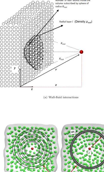
U(r) = Uwf(r) +Uf f(r), (2.4) U(r) = Nw X i=1 uAA_wf(|r−ri|) + Nf X i=1 uAA_{f f}(|r−ri|), (2.5) ≈ Z V uAA_wf(|r−r0|)ρwall(r0)dV + Z V uAA_{f f} (|r−r0|)ρ(r0)dV. (2.6)

Here,uAA_wf anduAA_{f f} are the inter-atomic separation dependent pair potentials that describe the wall-fluid and the fluid-fluid interactions, respectively. Nw and Nf are, respectively, the number of wall and fluid atoms that lie within the cutoff sphere around the position r,ri is the location of atom i, ρwall(r0) and ρ(r0) are, respectively, the wall and the fluid density in the volume elementdV andV is the volume circumscribed by the cutoff sphere. For spherical, non-polar LJ type spherical molecules,uAA_wf anduAA_{f f} are the 12-6 Lennard-Jones (LJ) pair-potentials used in the MD simulation. In the quasi-continuum formulation, the wall-fluid and the fluid-fluid interaction energy is computed in terms of a density weighted integration of the inter-atomic pair potentials as shown in Figs. 2.2(a) and 2.2(b), respectively. Using the structural information of the wall, the integral representing the wall-fluid interaction energy Uwf can be evaluated easily. Such density

based wall-fluid interaction models were originally discussed by Steele [50, 51] and are widely used in the simulation of gas physisorption phenomena. Two well-known examples of such potentials for planar walls are the LJ 9-3 wall and LJ 10-4 potentials. The development of the quasi-continuum wall-fluid potential models for cylindrical and spherical shape confinement and many industrially important heterogeneous/patterned walls are discussed in Refs. [50–56]. For LJ type confined fluids,Uwf is independent of the fluid density and depends only on the wall structure and the wall-fluid interaction parameters. Also, as the structure of the wall does not change,Uwf is computed just once in the EQT formulation.

We now discuss the evaluation of integral representing the fluid-fluid interaction energy

Uf f(r) = Z

V

(21)

(Density ρ_wall)

(a) Wall-fluid interactions

(Density ρ(ri))

(b) Fluid-fluid interactions

Figure 2.2: Computation of the wall-fluid and fluid-fluid interaction energy in the quasi-continuum formula-tion. (Figure courtesy of Mohammad Hossein Motevaselian).

(22)

Unlike wall-fluid potential integral, the computation of the fluid-fluid interaction energy integral is compli-cated and needs to be performed carefully. As fluid-fluid interaction energy is a function of the unknown fluid densityρ(r), integral given by Eq. (2.7) is computed iteratively in the EQT formulation, until a self-consistent density and potential profiles are obtained. Due to the highly inhomogeneous nature of the fluid density near the interface and the singular nature of the inter-molecular potentialuAA_{f f} (r) as r→0, the evaluation of this integral leads to numerical singularity. This numerical singularity is a classic example of the length and time scale mismatch complexity that can arise while developing multiscale models. The physical origin of this singularity is the implicit use to the mean-field approximation (MFA) in writing the quasi-continuum expression for the fluid-fluid interaction energy (Eq. (2.7)). In MFA, two-particle correlation, g(|r−r0|), which specifies the relative probability of finding two particles at a distance|r−r0|is assumed to be 1. At very small distances (|r−r0| →0), due to finite size and excluded volume effects this probability is zero. One possible approach to avoid this problem is to develop models forg(|r−r0|), which is the approach taken in integral equation theories (IET) [23]. Although, a great deal of progress has been made in developing pair-correlations for real fluids, the IET framework is mathematically quite complex to implement and suf-fers from the “closure” problem. In a very recent extension of EQT for studying thermodynamic properties of confined fluids [24], pair-correlation models based on hard-sphere radial distribution function are used to compute this integral. In this work, we use an alternative strategy of replacing the singular uAA_{f f} by a truncated soft-core potentialut_{f f} and compute theUf f as

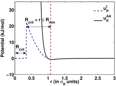
Uf f(r) = Z V utf f(|r−r0|)ρ(r0)dV, (2.8) whereut_{f f}(r) is defined as ut_{f f}(r) =            0 r≤Rcrit b0+b1r+b2r2 Rcrit< r≤Rmin uAA_{f f}(r) r > Rmin (2.9)

A schematic comparison of uAA_{f f} and ut_{f f} is shown in Fig. 2.3. It can be observed that ut_{f f} is exactly same as uAA_{f f} until r=Rmin, has a softer second-order polynomial repulsive form betweenRcrit and Rmin

and becomes zero for r ≤ Rcrit. Rmin and Rcrit are two coarse-graining parameters which define the softer repulsive region and the zero potential core, respectively. The coefficientsb0,b1 andb2 of the softer polynomial repulsive potential are calculated by enforcing the continuity of the potential and its first and second derivative atRmin. The functional form of the softer repulsive potential is an ansatz and lacks any

(23)

0 0.5 1 1.5 2 2.5 3 −10 0 10 20 30 Potential (kJ/mol) r (in σ ff units) ut ff uAA ff R crit R crit < r ≤ Rmin

Figure 2.3: Comparison ofuAA_{f f} (r) andut_{f f}(r). σf f is the fluid atomic diameter.

fundamental derivation. The parameters Rmin and Rcrit are obtained using the PMF matching technique

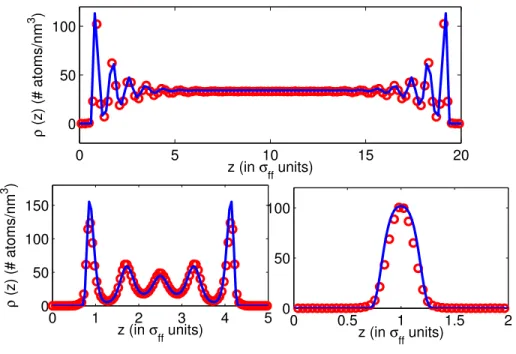
that matches the total interaction energy U(r) of the confined fluid as obtained from the quasi-continuum potentials with that obtained from all-atom MD (AA-MD) simulation. For a given thermodynamic state, PMF matching requires one AA-MD simulation to parameterize the quasi-continuum potentials. We discuss the PMF matching algorithm in detail in Sec. 2.2.4. Once the quasi-continuum potentials are parameterized, they can be used in EQT to predict the density and potential profiles of fluids confined inside different width channels which are loaded at the same thermodynamic state. Figure 2.4 shows the comparison of the density profile of the LJ oxygen atoms confined inside different width slit-shape channels as obtained from EQT (solid line) and MD simulations (open circle). It can be observed that the results obtained from EQT capture both the interfacial (non-continuum inhomogeneous behavior) and the bulk (continuum behavior) structure of the confined LJ oxygen. Further, as EQT is a continuum-based approach, it is several orders of magnitude faster than MD simulation. The development of transferable quasi-continuum potential models for confined LJ type fluids is discussed in detail in Ref. [48].

We wish to mention that though the EQT formulation is discussed for fluids confined inside slit-shape nanochannels, it can be straightforwardly applied to other geometries such as a carbon nanotube (CNT). In addition, for confinements where the total potential varies in two or three dimensions, the EQT framework can be extended by considering a multi-dimensional form of Eq. (2.1). With the successful application of EQT for spherical, non-polar LJ type fluids, we now address the first research objective of extending the EQT framework to study the structure of poly-atomic molecules in confined environments.

(24)

0 1 2 3 4 5 0 50 100 150 z (in σ ff units) ρ (z) (# atoms/nm 3 ) 0 5 10 15 20 0 50 100 z (in σ ff units) ρ (z) (# atoms/nm 3 ) 0 0.5 1 1.5 2 0 50 100 z (in σ ff units)

Figure 2.4: Comparison of density profile from EQT (solid line) and MD simulation (open circle). σf f is the

fluid atomic diameter.

2.2 EQT for poly-atomic fluids

For poly-atomic molecules, the molecular interactions in MD are typically described through the interaction potentials that define the interactions between the constituent atoms and depend on the internal coordinates of each molecule. To develop the quasi-continuum potentials, we first develop coarse-grained single-site (CGSS) pair-potentials that describe an effective interaction between the two molecules (averaging out the internal degrees of freedom) and then use them in the continuum approximation (Eq. (2.6)) to compute the total interaction potential of the confined poly-atomic fluid. We take 3-site carbon-dioxide (CO2) molecule as an example, which is a linear molecule with both LJ and electrostatic interactions present, and discuss the development of CGSS pair-potentials and quasi-continuum potential models that predict the correct microstructure of CO2in confined environments. We coarse-grain CO2 as a single-site point particle placed at its center-of-mass (COM) position. Over the years, several potential models have been proposed to represent carbon dioxide [2, 57–59]. Most of these models can be categorized into two sub-groups: 1) All atom (AA) site-site potentials in which carbon dioxide is modeled as a rigid two/three site Lennard-Jones (LJ) molecule with quadrupole moment either stated explicitly or decomposed into partial charges. These models are computationally quite expensive, but provide a fairly accurate description of the structural properties of carbon dioxide, both in the bulk state and under nanoscale confinement. 2) Single-site LJ

(25)

0 0.4 0.8 1.2 1.6 2 2.232 0 20 40 60 80 z (nm) ρ (z) (# molecules/nm 3) CGSS Bulk AA Model Shoulder Peak H = 2.232 nm, T = 323 K, P = 10.1 MPa

Figure 2.5: COM density of confined CO2 from a bulk CGSS potential model [1](broken line) and a 3-site AA potential model [2] (solid line).

type potentials which ignore the microscopic structural information related to the shape of the molecule and model CO2 as a spherical and isotropic single-site molecule. There exist several COM position based single-site potential models that provide a fairly accurate description for CO2 in the bulk state [1, 59]. We first show that CGSS bulk potentials cannot be used to predict the correct microstructure of CO2in confined environments. Figure 2.5 shows the comparison of the 1-D COM density, ρ(z), for CO2 confined inside a 2.232 nm wide graphite slit nanochannel, as obtained by using a bulk CGSS potential [1] and a AA 3-site potential model [2] in a MD simulation. It can be observed that the density profile obtained from the bulk CGSS model over-predicts the density layering and completely fails to predict the splitting of the first peak into a second sub-layer (shoulder peak) near the confining surface. This confinement induced splitting of the first density layer is a consequence of the shape and the orientation of the CO2 molecules which is absent in the CGSS models developed for the bulk state. To develop CGSS pair potentials for nanoconfined poly-atomic fluids, the geometric shape and the orientation information must be considered. We now discuss the development of the CGSS pair-potentials to describe wall-fluid and fluid-fluid interactions for CO2 in confined environments.

2.2.1 CGSS Potentials: Functional Form

The specification of the functional form of the interaction potential is one of the most important and chal-lenging tasks in the process of coarse-graining [28, 29]. Typically, the specification of the functional form

(26)

is guided by the understanding of the physics of the problem. To propose the functional form for CGSS wall-CO2 and CO2-CO2 interaction potentials, we first discuss the microstructure of CO2 molecules under nanoscale confinement. Figures 2.6(a) and 2.6(b) show the COM density profile, ρ(z), and the molecular orientation profile,Sθ, respectively, for CO2confined inside a 2.232 nm wide graphite slit nanochannel. The molecular orientation is computed using the order parameterSθdefined as

Sθ=3hcos 2_θ_{i −}₁

2 (2.10)

Here,θis the angle between the molecular axis and a normal vector through the walls and angular brackets denote ensemble averaging. The order parameter takes a value of –0.5 if molecules are aligned parallel to the wall, a value of 1 if the molecules are aligned perpendicular to the wall, and a value of 0 if they are randomly oriented. Further, to understand the effect of the wall-fluid and the fluid-fluid interactions separately, we divide the confining geometry into two regions. The region up to 0.5 nm from the walls (z ≤ 0.5 nm and

z≥1.732 nm), where the wall-fluid interactions are the dominant interactions, is defined as the interfacial region and the remaining region is defined as the central region of the nanochannel. It can be observed from Figs. 2.6(a) and 2.6(b) that the two sub-layers in the first peak have a different preferred molecular orientation. In the first sub-layer, the order parameter is less than zero (Sθ ≈ –0.4) and molecules are aligned parallel to the wall, while in the second sub-layer the order parameter is greater than zero (Sθ≈0.2) indicating that the molecules are rotated with respect to the wall. Under high pressure (or high density) nanoscale confinement, the molecules arrange themselves into layers which are rotated relative to each other. This type of arrangement occurs because of the linear shape of the carbon dioxide molecule and results in the most efficient packing under confinement. To capture this orientation dependent arrangement of molecules in the interfacial region, we use piecewise interaction functions and define the wall-CO2interaction potential as uCGSS_wall_-_CO 2(r) =            uLJ(r, σ1, 1) r≤Rtrans a0+a1r+a2r2+a3r3 Rtrans< r≤Rtrans+ ∆ c1uLJ(r, σ1, 1) +c2uLJ(r, σ2, 2) r > Rtrans+ ∆ (2.11)

whereuLJ(r, σi, i) is defined as

uLJ(r, σi, i) = 4i _σi r 12 −σi r 6 , i= 1,2. (2.12)

Here,ris the distance between the wall atom and the CG CO2molecule. σiandi are the distance and the energy parameters, respectively. The first region is a 12-6 LJ potential up toRtransto model the interaction

(27)

0 0.4 0.8 1.2 1.6 2 2.232 −0.5 0 0.5 1 z (nm) Sθ 0 0.4 0.8 1.2 1.6 2 2.232 0 20 40 60 ρ (z) (# molecules/nm 3) (a)

Second sub−layer (Shoulder Peak)

(b) Central Region Central Region Interfacial Region Interfacial Region 0 0.4 0.8 1.2 −2 −1 0 1 2 r (nm) Potential (kJ/mol) (c) ∆ 0 < r ≤ R trans r ≥ R trans+∆ 0 0.2 0.4 0.6 0.8 1 1.2 0 30 60 90 A n g le ( o) r COM (nm) !₁,!₂ " (d) ! " # $ % !" #"

Figure 2.6: (a) COM density profile, ρ(z), (b) Molecular orientation profile, Sθ, (c) Functional form of

uCGSSwall-CO2(r) andu

CGSS

CO2-CO2(r), and (d) Relative orientation profile of CO2confined inside a 2.232 nm wide

(28)

of the wall atoms with the CO2molecules in the first sub-layer. The second region is a linear superposition of two 12-6 LJ potentials, and operates at separation distances greater thanRtrans+∆ to model the interaction

of the wall atoms with the CO2 molecules in the second sub-layer. c1 andc2 are two constants that control the contribution of the two 12-6 LJ potentials in the second region. The two regions are connected by a polynomial bridge function of width ∆. The coefficientsa0, a1, a2anda3of the bridge function are computed to ensure smooth transition of the potential (continuity of the potential and its first derivative) at Rtrans

andRtrans+ ∆. A sketch of the functional form is given in Fig. 2.6(c).

To define the fluid-fluid interactions, we plan to use the same functional form as proposed for the wall-CO2 interactions. Although this molecular orientation analysis guides us to define the functional form, it does not provide any information on the relative orientation of the two fluid molecules, which could be different in the interfacial and the central region. This information on the relative orientation is required to understand if one uniform fluid-fluid potential could be used across the entire length of the confinement. If the relative orientation profile is different in the two regions, then one would have to define a separate fluid-fluid interaction potential for each region. Figure 2.6(d) shows the relative orientation profile of CO2 molecules in the interfacial (solid line) and the central (broken line) region of the confinement. The relative orientation is defined in the COM coordinates rCOM, θ1, θ2 and φ(see inset of Fig. 2.6(d)). rCOM is the separation between the COM of the two molecules,θis the angle made by the molecular axis of each molecule with therCOM andφis the dihedral angle between the two planes defined by therCOM and the molecular axis for each molecule. It can be observed that the relative orientation profile in the interfacial region is not significantly different from that in the central region (∆θ1'7o, ∆θ2'7o, ∆φ'3o; ∆θ1, ∆θ2and ∆φ are the difference between the values ofθ1,θ2 andφin the interfacial and the central region, respectively). Thus, we specify one uniform interaction potential and define the CO2-CO2interaction potential as

uCGSS_CO 2-CO2(r) =            uLJ(r, σ1, 1) r≤Rtrans a0+a1r+a2r2+a3r3 Rtrans< r≤Rtrans+ ∆ c1uLJ(r, σ1, 1) +c2uLJ(r, σ2, 2) r > Rtrans+ ∆ (2.13)

Here, r is the distance between the two CG CO2 molecules. All other functions and parameters have the same meaning as defined above foruCGSS_wall_-_CO₂.

2.2.2 CGSS Potentials: Parameterization

Once the functional form is specified, the next step is the parameterization of the potential to reproduce the property of interest, commonly referred to as the target function in the coarse-graining literature. We

(29)

parameterizeuCGSSwall-CO2 andu

CGSS

CO2-CO2 to reproduce the potential of mean force (PMF) of the confined fluid.

The PMF variation,Ui(r), of a particle iat positionris computed as [60]

Ui(r) = Ui(ro)− Z r

ro

hFi(r0)idr0 (2.14)

Here, hFi(r)iis the mean force that acts on particle i (at position r) due to its interaction with all other particles. Ui(ro) is the value of the potential at a reference position ro. For semi-infinite slit nanochannels considered in this work, the reference positionrois taken to be the center of the nanochannel, i.e.,ro(x, y, z) = (x, y, H/2); H is the slit width. Also, since the slit is infinite in xand y directions, only the variation in the z direction is relevant. To parameterize the potentials for a given thermodynamic state, we first run an AA-MD simulation and compute the wall-fluid PMF (PMF profile due to the wall-fluid interactions),

U_wallAA_-_CO

2(z), and the fluid-fluid PMF (PMF profile due to the fluid-fluid interactions),U

AA

CO2-CO2(z), of the

confined fluid. The wall-fluid and the fluid-fluid PMF are computed by decomposing the total force that acts on a molecule as contributions from the wall-fluid and the fluid-fluid interactions, respectively. To find the contribution from the wall-fluid (or fluid-fluid) interactions, we take AA-MD equilibrium trajectories as input and recompute the total force on each molecule due to the wall-fluid (or fluid-fluid) interactions alone. This can be performed using the rerun option in the mdrun program of the simulation package GROMACS. [61]

U_wallAA_-_CO₂(z) andU_COAA₂_-_CO₂(z) are computed as

UwallAA-CO2(z) = U AA wall-CO2(zo)− Z z zo hFwallAA-CO2(z 0_)i_dz0 _(2.15) U_COAA₂_-_CO₂(z) = U_COAA₂_-_CO₂(zo)− Z z zo hF_COAA₂_-_CO₂(z0)idz0 (2.16)

Here, hFwallAA-CO2(z)i and hF

AA

CO2-CO2(z)i are the mean force experienced by the molecules at position z

(molecules whose COM lie in the bin [z,(z+ ∆z)]) due to the wall-fluid and the fluid-fluid interactions, respectively. U_wallAA_-_CO

2(zo) andU

AA

CO2-CO2(zo) are the reference wall-fluid and fluid-fluid potentials at position

zo =H/2. UwallAA-CO2(z) and U

AA

CO2-CO2(z) are the target wall-fluid and fluid-fluid PMF profiles, which we

want to reproduce with uCGSS_wall_-_CO

2 and u

CGSS

CO2-CO2, respectively. The CG wall-fluid and fluid-fluid PMF

profiles are computed following the same procedure as discussed above for the computation of the target PMF profiles. First, the total force experienced by each CG CO2 molecule (CO2 is coarse-grained as a spherical bead placed at its COM position) due to the CG wall-fluid and fluid-fluid interactions (defined by

(30)

uCGSSwall-CO2(r) andu CGSS CO2-CO2(r)) is computed, i.e., F_wallCG_-_CO₂(r_iAA) = Nj X j=1 −d dr u CGSS wall-CO2(|r AA i −r AA j |) (2.17) F_COCG 2-CO2(r AA i ) = Nj X j=1 −d dr u CGSS CO2-CO2(|r AA i −r AA j |) (2.18)

Here, rAA_i andr_jAA are the COM position of the moleculesi andj, as obtained from AA-MD trajectories and Nj is the number of molecules within the cutoff sphere around the molecule i. F_wallCG_-_CO₂(rAA_i ) and

F_COCG₂_-_CO₂(r_iAA) are the total force that acts on the molecule i (at positionrAA_i ) due to the wall-fluid and the fluid-fluid interactions, respectively. This step can be performed using the table [62] and rerun option in the mdrun program of the simulation package GROMACS. Then, the CG wall-fluid PMF,UwallCG-CO2(z),

and the CG fluid-fluid PMF,UCOCG2-CO2(z), are computed as

U_wallCG_-_CO 2(z) =U CG wall-CO2(zo)− Z z zo hF_wallCG_-_CO 2(z 0_)i_dz0 _(2.19) UCOCG2-CO2(z) =U CG CO2-CO2(zo)− Z z zo hFCOCG2-CO2(z 0_)i_dz0 _(2.20) Here,hF_wallCG_-_CO 2(z)iandhF CG

CO2-CO2(z)iare the mean force experienced by the molecules at positionzdue to

the CG wall-fluid and fluid-fluid interactions, respectively. U_wallCG_-_CO

2(zo) andU

CG

CO2-CO2(zo) are the reference

wall-fluid and fluid-fluid potentials at positionzo=H/2. This process (Eqs. (2.17) to (2.20)) is repeated by

varying the parameters of the CGSS potentials, uCGSS_wall_-_CO₂ and uCGSS_CO₂_-_CO₂, until a good match between the CG and the target PMF profiles is obtained. The parameterization procedure is summarized in Algorithm 1. Figures 2.7(a) and 2.7(b) show the comparison of the CG wall-fluid and fluid-fluid PMF profiles (solid line)

Algorithm 1Parametrization of CGSS wall-fluid and fluid-fluid interaction potential.

1: Perform an all-atom molecular dynamics (AA-MD) simulation and compute U_wallAA_-_CO₂ and U_COAA₂_-_CO₂

using Eqs. (2.15) and (2.16), respectively.

2: Take initial guess for [σ1,1,σ2, 2,Rtrans, ∆,c1,c2] for bothuCGSSwall-CO2 andu

CGSS CO2-CO2.

3: Take AA-MD simulation trajectories and use Eqs. (2.17) to (2.20) to computeUwallCG-CO2 andU

CG CO2-CO2.

4: Obtain [σ1, 1,σ2,2,Rtrans, ∆,c1,c2] by solving the non-linear equations

U_wallCG_-_CO 2−U AA wall-CO2= 0 and U CG CO2-CO2−U AA CO2-CO2 = 0 .

with their respective target PMF profiles (open circle) for supercritical carbon dioxide (T = 323 K and P = 10.1 MPa) confined inside a 2.232 nm wide graphite slit nanochannel. The parameters used in the CGSS potentials are reported in Table 2.1. It can be observed that the CG wall-fluid and fluid-fluid PMF profiles match well with their respective target PMF profiles. The proposed functional form foruCGSS_wall_-_CO₂

(31)

0 0.4 0.8 1.2 1.6 2 2.232 −1 0 1 2 3 z (nm) Potential (K B T) 0 0.4 0.8 1.2 1.6 2 2.232 −5 0 5 z (nm) Potential (K B T) (a) (b)

Figure 2.7: Comparison of (a) CG wall-fluid PMF profile,U_wallCG_-_CO₂, (solid line) and (b) CG fluid-fluid PMF profile, U_COCG₂_-_CO₂, (solid line) with their respective target AA-MD PMF profiles (open circle) for carbon dioxide confined inside a 2.232 nm wide graphite slit nanochannel at T = 323 K and P = 10.1 MPa. The reference potential value is subtracted from each PMF profile while plotting.

Table 2.1: Parameters of CGSS wall-fluid and fluid-fluid interaction potentials.

Thermodynamic Potential σ1 1 σ2 2 Rtrans ∆ c1 c2

State (nm) (KJ/mol) (nm) (KJ/mol) (nm) (nm)

T=323K P=10.1MPa uCGSSwall-CO2 0.335 0.45 0.405 0.55 0.345 0.05 0.55 0.45 uCGSS_CO 2-CO2 0.335 1.15 0.405 1.75 0.375 0.03 0.50 0.50 T=348K P=9.05MPa uCGSSwall-CO2 0.335 0.45 0.405 0.55 0.345 0.05 0.55 0.45 uCGSS_CO 2-CO2 0.335 1.15 0.405 1.70 0.375 0.03 0.50 0.50 T=308K P=5.5MPa uCGSSwall-CO2 0.335 0.45 0.405 0.55 0.345 0.05 0.55 0.45 uCGSS_CO 2-CO2 0.335 1.05 0.405 1.95 0.40 0.03 0.50 0.50 T=323K P=1.01MPa uCGSSwall-CO2 0.335 0.45 0.405 0.55 0.365 0.05 0.55 0.45 uCGSS_CO 2-CO2 0.335 1.15 0.405 1.65 0.40 0.03 0.50 0.50

(32)

captures the two minima in the wall-fluid PMF quite accurately. These two minima cause the splitting of the density profile in the interfacial region into two sub-layers. uCGSS_CO

2-CO2 also captures the minima in the

fluid-fluid PMF profile quite accurately. These minima positions correspond to the density peaks in the central region of the channel. There is a small error in the magnitude of the CG fluid-fluid PMF profile in the region up to 0.3 nm from the walls. Due to the highly repulsive nature of the wall-fluid PMF in this region (U_wallCG_-_CO₂(z) > 5 KBT; KB is the Boltzmann constant), this error does not effect the structural prediction in the interfacial region. It is important to understand that this parameterization procedure ensures that given a set of equilibrium trajectories, uCGSS_wall_-_CO₂ and uCGSS_CO₂_-_CO₂ will reproduce the wall-fluid and the fluid-fluid PMF profiles of the confined fluid, respectively. It does not guarantee that given any random initial configuration, these potentials would evolve the system to its equilibrium configuration the same way as AA-MD simulation. This issue is checked later when we use these potentials to perform CG-MD simulations.

2.2.3 CGSS Potentials: Transferability

To check the transferability of the functional form ofuCGSS_wall_-_CO₂ and uCGSS_CO₂_-_CO₂, they were parameterized for four different thermodynamic states (T = 323 K, P = 10.1 MPa; T = 323 K, P = 1.01 MPa; T = 348 K, P = 9.05 MPa; T = 308 K, P = 5.5 MPa). The first two states are chosen to check the transferability of the functional form to high and low pressure confinements. The last two states are representative of high pressure confinement at supercritical temperatures. During parameterization, the variation of the coarse-graining parameters was studied to obtain their functional dependence with the thermodynamic variables and associate a physical meaning where ever possible. While parameterizing the wall-fluid interaction potential,

uCGSS_wall_-_CO₂, for high-pressure confinements (pressure values for which the first layer splits into two sub-layers), it was observed that the values of the parametersσ1andσ2 were quite close to the distance values at which the two minima occur in the wall-CO2 PMF profile. For the three high-pressure states (P ≥ 5.5 MPa) considered in this work, the first and the second minima occur at approximately 0.335 nm and 0.405 nm away from the wall, respectively. Hence, to parameterizeuCGSSwall-CO2, the valuesσ1= 0.335 nm andσ2= 0.405

nm were used and they worked well in all the three high-pressure thermodynamic states. Interestingly, the usage of the same values (σ1= 0.335 nm andσ2= 0.405 nm) also worked fine in the parameterization of the fluid-fluid interaction potential,uCGSS_CO

2-CO2, for these high-pressure states. Also, foru

CGSS

wall-CO2, it was observed

that once it is parameterized for a high-pressure state (T = 323 K, P = 10.1 MPa), only the coarse-graining parameterRtransneeds to be changed to re-parameterize it for a low-pressure state at the same temperature (T = 323 K, P = 1.01 MPa). The potentials were not found to be physically sensitive to the coarse-graining

(33)

0 0.4 0.8 1.2 1.6 1.85 −1 1 3 5 z (nm) Potential (K B T) 0 0.4 0.8 1.2 1.6 2 2.232 −1 0 1 2 3 4 UCG_CO 2−CO2 z (nm) Potential (K B T) 0 0.4 0.8 1.2 1.6 2 2.232 −5 0 5 z (nm) Potential (K B T) 0 0.4 0.8 1.2 1.6 2 2.232 −5 0 5 z (nm) Potential (K B T) UCG_wall−CO 2 0 0.5 1 1.5 1.85 −5 0 5 z (nm) Potential (K B T) 0 0.4 0.8 1.2 1.6 2 2.232 −1 0 1 2 3 z (nm) Potential (K B T) H = 2.232 nm T = 348 K, P = 9.05 MPa H = 1.85 nm T = 308 K, P = 5.5 MPa H = 1.85 nm T = 308 K, P = 5.5 MPa H = 2.232 nm T = 323 K, P = 1.01 MPa H = 2.232 nm T = 323 K, P = 1.01 MPa H = 2.232 nm T = 348 K, P = 9.05 MPa

Figure 2.8: Comparison of the CG wall-fluid PMF,UwallCG-CO2, (left) and the CG fluid-fluid PMF,U

CG CO2-CO2,

(right) profiles obtained from CGSS potentials (solid line) with their respective target AA-MD PMF profiles (open circle) at different thermodynamic states. The reference potential value is subtracted from each PMF profile while plotting.

parameters ∆, c1 andc2, whose variations were mostly considered to fine tune the results. c1 = c2 = 0.5 and ∆ value in the range 0.03 to 0.05 nm were found to be working fine for all the four thermodynamic states considered in this study. Figure 2.8 shows the comparison of the CG wall-fluid PMF, U_wallCG_-_CO₂, (left) and the CG fluid-fluid PMF, U_COCG₂_-_CO₂, (right) profiles obtained from CGSS potentials (solid line) with their respective target PMF profiles (open circle) at different thermodynamic states. The parameters for the CGSS potentials are obtained following the procedure outlined in Algorithm 1, and are reported in Table 2.1. It can be observed that the proposed functional form of uCGSS_wall_-_CO

2 performs well for all the

thermodynamic states and reproduces the wall-fluid PMF quite accurately. The functional form ofuCGSS_CO

2-CO2

performs better for high pressure (or density) states than for low pressure states. At high densities, short range inter-molecular repulsions are typically the dominant interactions, and uCGSS_CO

2-CO2, which is designed

(34)

long range electrostatic interactions also become important anduCGSSCO2-CO2 does not capture these long range

effects quite efficiently. The performance of uCGSS_CO

2-CO2 for low density confinements could be improved by

supplementing its functional form with a slowly varying function (e.g. a Gaussian or a smaller exponent LJ potential) that can capture the long range effects more efficiently.

2.2.4 Quasi-continuum potential models for Carbon Dioxide

We useuCGSSwall-CO2andu

CGSS

CO2-CO2to develop the quasi-continuum potential models for confined carbon dioxide,

i.e., U(r) =Uwall-CO2(r) +UCO2-CO2(r), (2.21) Uwall-CO2(r)≈ Z Ω uCGSSwall-CO2(|r−r 0_|)_ρwall₍_r0₎_dr0_, _(2.22) UCO₂-CO2(r)≈ Z Ω uCGSSCO2-CO2(|r−r 0_|)_ρCO 2(r 0₎_dr0_. _(2.23)

Here,ρwall andρCO2 are the wall and the fluid density, respectively. Uwall-CO2(r) andUCO2-CO2(r) are the

wall-fluid and the fluid-fluid interaction energy, respectively. The wall-fluid interaction energy, Uwall-CO2

(Eq. (2.22)), is computed by assuming the graphite surface as a continuum graphene layer with ρwall = 35

atoms/nm2 and an inter-layer spacing of 0.335 nm. Similar to LJ type fluids, fluid-fluid interaction energy,

UCO₂-CO2, is computed using a truncated softer repulsive core potentialu

t CO2-CO2 as UCO₂-CO2(r) ≈ Z Ω ut_CO₂_-_CO₂(|r−r0|)ρCO₂(r0)dr0 (2.24) whereutCO2-CO2(r) is defined as ut_CO₂_-_CO₂(r) =            0 r≤Rcrit b0+b1r+b2r2 Rcrit< r≤Rmin uCGSS_CO₂_-_CO₂(r) r > Rmin (2.25)

RminandRcritdefine the softer repulsive region and the zero potential core, respectively. The coefficientsb0,

b1 andb2are computed by enforcing the continuity of the softer potential and its first and second derivative at Rmin. The parameters Rmin and Rcrit are also obtained through PMF matching algorithm, which is

summarized in Algorithm 2. The parameterization of the quasi-continuum fluid-fluid interaction potential (findingRmin andRcrit) is performed using the same AA-MD simulation data that is used to parameterize

(35)

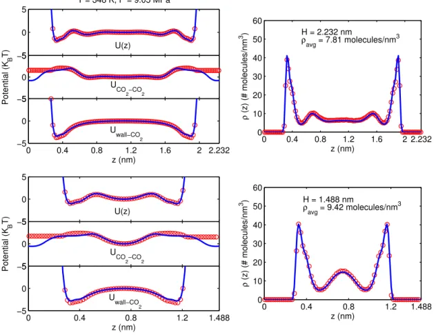
0 0.4 0.8 1.2 1.6 2 2.232 0 10 20 30 40 50 60 z (nm) ρ (z) (# molecules/nm 3 ) 0 0.4 0.8 1.2 1.488 0 10 20 30 40 50 60 z (nm) ρ (z) (# molecules/nm 3 ) −5 0 5 T = 348 K, P = 9.05 MPa −5 0 5 Potential (K B T) 0 0.4 0.8 1.2 1.6 2 2.232 −5 0 5 z (nm) −5 0 5 −5 0 5 Potential (K B T) 0 0.4 0.8 1.2 1.488 −5 0 5 z (nm) U(z) U(z) U_CO 2−CO2 U_wall−CO 2 U_CO 2−CO2 U wall−CO 2 H = 1.488 nm ρ avg = 9.42 molecules/nm 3 H = 2.232 nm ρ_avg = 7.81 molecules/nm3

Figure 2.9: Comparison of the COM density and potential profiles obtained by using the quasi-continuum potentials in EQT (solid line) with those obtained from AA-MD simulations (open circle) for supercritical carbon dioxide (T = 348 K and P = 9.05 MPa) confined inside H = 2.232 nm and H = 1.488 nm wide graphite slit nanochannels. The reference potential value is subtracted from each PMF profile while plotting.

ρCO2(r) is needed to perform this optimization. Once the quasi-continuum potential is optimized for a given

thermodynamic state, it is used in EQT to predict the COM density and potential profiles of CO2in different size nanochannels. Figure 2.9 shows the comparison of the COM density and potential profiles obtained by using the quasi-continuum models in EQT (solid line) with the AA-MD simulation results (open circle) for supercritical carbon dioxide (T = 348 K and P = 9.05 MPa) confined inside a 2.232 nm and 1.488 nm wide graphite slit nanochannels. The parameters used inuCGSS_wall_-_CO₂ and uCGSS_CO₂_-_CO₂ for this thermodynamic state are reported in Table 2.1. ParametersRmin and Rcrit used in ut_CO₂_-_CO₂ are reported in Table 2.2. It can be observed that the results obtained from EQT are in good agreement with those obtained from AA-MD simulations.

(36)

Algorithm 2Parametrization of fluid-fluid quasi-continuum potential.

1: Input: ρCO₂(r) and target PMF,UAA(r), from AA-MD simulation.

2: Compute the wall-fluid PMF, Uwall-CO2(r), using Eq. (2.22).

3: Take initial guess for Rmin andRcrit.

4: Compute the fluid-fluid PMF, UCO₂-CO2(r), usingρCO2(r) andu

t

CO2-CO2(r) in Eq. (2.24).

5: Calculate U(r) =Uwall-CO2(r) +UCO2-CO2(r) (Eq. (2.21)).

6: ObtainRmin andRcritby solving the non-linear equation U(Rmin, Rcrit, r) -UAA(r) = 0.

Table 2.2: Softer repulsive core parameters Thermodynamic State Rcrit Rmin

(nm) (nm) T=323K, P=10.1MPa 0.174 0.364 T=323K, P=1.01MPa 0.201 0.364 T=348K, P=9.05MPa 0.174 0.362 T=308K, P=5.50MPa 0.164 0.365

2.3 COM density profiles from EQT

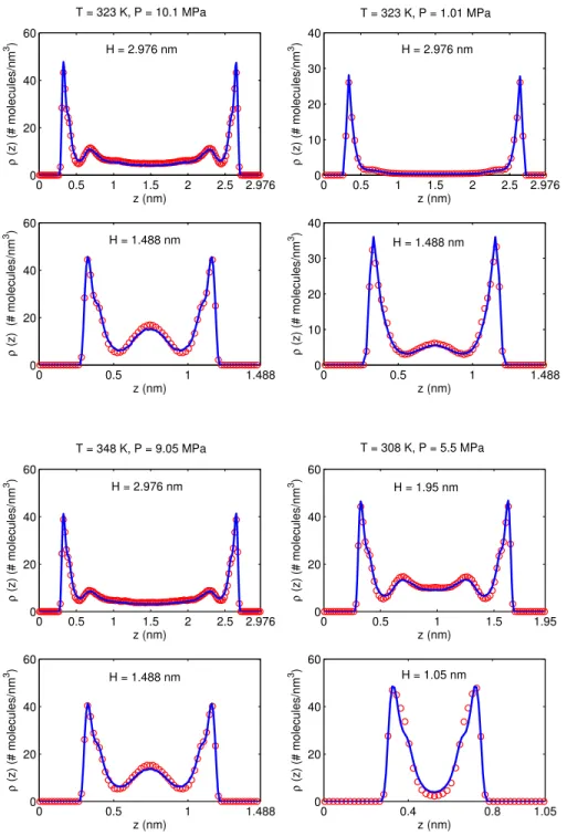
We now use the quasi-continuum potentials in EQT to predict the COM density profile of CO2 confined inside different width (1.05 to 3.72 nm) graphite slit nanochannels. Figure 2.10 shows the comparison of the COM density profiles at a high and a low pressure confinement state (P = 10.1 MPa and 1.01 MPa; T = 323 K). For both these states the potentials are parameterized using the AA-MD data ofH = 2.232 nm wide graphite slit. The parameters are reported in Tables 2.1 and 2.2. It can be observed that the density profiles obtained from EQT (solid line) match well with those obtained from AA-MD simulations (open circle). For bigger nanochannels (H = 3.72 and 2.976 nm), the potentials capture both the density layering in the interfacial region and the bulk like behavior in the central region of the nanochannels. For smaller nanochannels (H = 1.488 and 1.116 nm), confinement makes the density inhomogeneous across the entire length of the nanochannel, which is also captured well with these potentials. At low pressure (low density) confinements, most of the fluid confinement occurs near the wall. Also, the density layer in the interfacial region does not split into two sub-layers and resembles like that of confined simple LJ type fluids. Figure 2.11 shows the COM density profiles at two different supercritical temperature states (T = 348 K, P = 9.05 MPa and T = 308 K, P = 5.5 MPa) as obtained from EQT. For T = 348 K state, the potentials are parameterized using the AA-MD data ofH = 2.232 nm wide slit, while for T = 308 K state, AA-MD data ofH = 1.850 nm wide slit is used to parameterize the potentials. The parameters are reported in Tables 2.1 and 2.2. Again, the results obtained from EQT are in good agreement with those obtained from AA-MD simulations. The general structural behavior at these two states looks quite similar to each other.

Multiscale models for structure and dynamics of confined fluids