Working Paper 08-13 Departamento de Estadística Statistic and Econometric Series 05 Universidad Carlos III de Madrid
March 2008 Calle Madrid, 126
28903 Getafe (Spain)
Fax (34-91) 6249849
A SEMI-PARAMETRIC MODEL FOR CIRCULAR DATA BASED
ON MIXTURES OF BETA DISTRIBUTIONS
∗Jose Antonio Carnicero
1, Michael Peter Wiper
2Abstract
This paper introduces a new, semi-parametric model for circular data, based on mixtures of shifted, scaled, beta (SSB) densities. This model is more general than the Bernstein polynomial density model which is well known to provide good approximations to any density with finite support and it is shown that, as for the Bernstein polynomial model, the trigonometric moments of the SSB mixture model can all be derived.
Two methods of fitting the SSB mixture model are considered. Firstly, a classical, maximum likelihood approach for fitting mixtures of a given number of SSB components is introduced. The Bayesian information criterion is then used for model selection. Secondly, a Bayesian approach using Gibbs sampling is considered. In this case, the number of mixture components is selected via an appropriate deviance information criterion.
Both approaches are illustrated with real data sets and the results are compared with those obtained using Bernstein polynomials and mixtures of von Mises distributions.
Keywords: circular data; shifted, scaled, beta distribution; mixture models; Bernstein polynomials JEL Classification: C14
1
Corresponding autor: Jose Antonio Carnicero Carreño, Universidad Carlos III Departamento de Estadística, C/ Madrid 126. 28903 Getafe (Madrid), España, e-mail: [email protected],
2 Corresponding autor: Michael P. Wiper, Universidad Carlos III, Departamento de Estadística, C/ Madrid
A semi-parametric model for circular data
based on mixtures of beta distributions
J.A. Carnicero and M.P. Wiper
April 3, 2008
Abstract
This paper introduces a new, semi-parametric model for circular data, based on mixtures of shifted, scaled, beta (SSB) densities. This model is more general than the Bernstein polynomial density model which is well known to provide good approximations to any density with finite support and it is shown that, as for the Bernstein poly-nomial model, the trigonometric moments of the SSB mixture model can all be derived.
Two methods of fitting the SSB mixture model are considered. Firstly, a classical, maximum likelihood approach for fitting mixtures of a given number of SSB components is introduced. The Bayesian information criterion is then used for model selection. Secondly, a Bayesian approach using Gibbs sampling is considered. In this case, the number of mixture components is selected via an appropriate de-viance information criterion.
Both approaches are illustrated with real data sets and the results are compared with those obtained using Bernstein polynomials and mixtures of von Mises distributions.
Keywords: circular data; shifted, scaled, beta distribution; mixture models; Bernstein polynomials.
AMS classification: 62H11.
1
Introduction
Problems where the data are angular directions occur in many different sci-entific fields such as biology (direction of movement of migrating animals),
meteorology (wind directions) and geology (directions of joints and faults). Also, phenomena that are periodic in time such as times of hospital ad-mittance for births or the times when crimes are committed may also be converted to angular data via a simple transformation modulo some period. Data of this type are commonly known as circular data and are usually rep-resented as points on the circumference of an unit circle or as angles,θ, where 0≤θ <2π radians, which represent the positive angle of rotation from some conveniently chosen origin.
It is clear that standard statistics are not always appropriate for circular data. For example, the pair of twenty four hour clock times 23:30 and 00:30 are closer to each other than are the pair 01:00 and 11:00 even though the numerical difference between the times is smaller in the second case. Also, the linear mean of the first pair of times is 12:00 which is clearly not a good measure of the average of the first pair of data. Instead, the “mean direction” is 24:00. A full review of circular moments and alternative statistics for circular data is contained in e.g. Mardia and Jupp (1999).
A number of parametric models for circular data have been developed using a variety of techniques. One approach is to “wrap” standard distribu-tions on the line onto the circle, that is to define the circular density at some angle, θ, to be the sum of the linear densities at θ, θ±2π, θ±4π, . . ., see e.g. Mardia and Jupp (1999), Jammalamadaka and Kozubowski(2003). Other models have been developed specifically for circular data. In particular, the von Mises distribution is an appropriate model for symmetric, unimodal, cir-cular data and has many similar properties to the normal distribution on the line, see e.g. Evans et al (2000).
Most models developed thus far for circular data are unimodal and sym-metric. However, in many cases, both multimodal and asymmetric data may be encountered. In such cases, non-parametric or semi-parametric mod-els might be considered. Fully non-parametric, kernel based approaches are considered by Fisher (1989). However, semi-parametric models will usually have more predictive power. Fern´andez-Dur´an (2004) has developed a semi-parametric model based on trigonometric sums and Mooney et al (2003) have considered mixtures of von Mises distributions. Both these approaches have certain disadvantages. In the first case, as noted by Ferreira et al (2005), the trigonometric sums approach can often fit wiggly densities which are un-realistic in practice and in the second case, as the von Mises distribution is symmetric, large numbers of terms may be needed to well approximate asymmetric data samples. In this paper, we introduce an alternative
semi-parametric, mixture model based on the use of shifted, scaled, beta (SSB) distributions.
The article is organized as follows. In Section 2 we define the SSB dis-tribution and and show how its circular moments may be calculated. We then introduce mixtures of SSB distributions and relate this mixture model to Bernstein polynomials which have been developed as an approach to esti-mating densities with support [0,1] by e.g. Vitale (1975), Petrone (1999a,b), Petrone and Wassermann (2002), Babu et al (2002) and Kakizawa (2004). In Section 3 we consider maximum likelihood estimation for the SSB mixture model and we fit our model to two, well known, real data sets, comparing the results obtained with mixtures of von Mises distributions and with Bernstein polynomials. In Section 4 we describe a Bayesian algorithm for estimating the predictive density and fit the model to a third group of real data. Finally, some concluding remarks and possible extensions are given in Section 5.
2
The SSB distribution and mixtures of SSB
distributions
2.1
The SSB distribution
Let θ be a random variable with support [0,2π). Then we shall say that θ has a SSB distribution with parameters 0 ≤ ν < 2π and α, β ∈ IN, denoted by θ∼ SSB(ν, α, β) if f(θ) = 1 (2π)α+β−1B(α,β)(2π+θ−ν)α−1(ν−θ)β−1 if 0≤θ < ν 1 (2π)α+β−1B(α,β)(θ−ν)α−1(2π+ν−θ)β−1 if ν ≤θ < 2π (1)
where B(α, β) = (α−1)!(β−1)!/(α+β−1)! is the beta function.
Clearly, we can represent the distribution of θ as the distribution of a shifted, scaled, beta distributed random variable, so that
θ = mod(2πX+ν,2π)
where mod(a, b) means a modulo b and X is a beta distributed random variable, X ∼ B(α, β), such that
f(x) = 1
B(α, β)x
The restriction in the definition of the SSB distribution thatα andβ are natural numbers is not strictly necessary. However, when fitting mixtures of SSB distributions to data, it is useful to include this restriction in order to avoid the possibility of fitting asymptotes which are unrealistic and would occur if α or β are below 1. Secondly, given that α and β are natural numbers, exact values for the circular or trigonometric moments of the SSB distribution can be derived as is shown in the following subsection.
2.2
Trigonometric moments of the SSB distribution
As noted in the introduction, the standard mean and other moments are not appropriate for circular random variables. Instead, for any circular random variable, θ, the p’th trigonometric moment is defined to be
μ
p = E
eipθ=E[cospθ] +iE[sinpθ] wherei=√−1
def=
ρp
cosμp+isinμp where
ρp =
E[cospθ]2+E[sinpθ]2 and (3)
μp = ⎧ ⎪ ⎪ ⎪ ⎪ ⎨ ⎪ ⎪ ⎪ ⎪ ⎩ tan−1 E[sinpθ]
E[cospθ] if E[sinpθ]>0 and E[cospθ]>0
tan−1 EE[cos[sinpθpθ]] +π if E[cospθ]<0 tan−1 E[sinpθ]
E[cospθ] + 2π if E[sinpθ]<0 and E[cospθ]>0
(4)
for p = 1,2, . . .. In particular, when p = 1, we write μ for μ1 and ρ for ρ1. Then, μ is the mean direction and ρ is the mean resultant length, see e.g. Mardia and Jupp (1999) for more details.
Similar sample equivalents can also be defined. Thus, given a sample of circular data,θ1, . . . , θn, then the circular mean, ¯θ, is defined as
¯ θ = ⎧ ⎪ ⎪ ⎪ ⎪ ⎪ ⎨ ⎪ ⎪ ⎪ ⎪ ⎪ ⎩ tan−1 n i=1sinθi n i=1cosθi if n i=1sinθi >0 and n i=1cosθi >0 tan−1 n i=1sinθi n i=1cosθi +π if n i=1cosθi <0 tan−1 n i=1sinθi n i=1cosθi + 2π if n i=1sinθi <0 and n i=1cosθi >0 (5)
and the sample mean resultant length, r, is
r= 1 n ⎛ ⎝ n i=1 sinθi 2 + n i=1 cosθi 2⎞ ⎠. (6)
The circular moments of an SSB random variable with origin zero can be calculated using Theorem 1.
Theorem 1. Let θ∼ SSB(0, α, β). Then, for p∈IN,
E[cos(pθ)] = 1 B(α, β) β−1 j=0 (−1)j β−1 j Ip(α+j−1) = 1 B(α, β) α−1 j=0 (−1)j α−1 j Ip(β+j−1) E[sin(pθ)] = 1 B(α, β) β−1 j=0 (−1)j β−1 j Jp(α+j−1) = 1 B(α, β) α−1 j=0 (−1)j+1 α−1 j Jp(β+j−1)
where Ip(0) =Jp(0) =Ip(1) = 0,Jp(1) =−2πp1 and for C >1,
Ip(C) = C 2 c=1 (−1)c−1 C! (C−2c+ 1)! 1 (2πp)2c Jp(C) = C+1 2 c=1 (−1)c C! (C−2c+ 2)! 1 (2πp)2c−1. ‡ The circular moments of a general SSB distribution can be derived as a simple corollary of Theorem 1.
Corollary 1. Let θ ∼ SSB(ν, α, β). Then, for p∈IN,
E[cos(pθ)] = 1 B(α, β) ⎧ ⎨ ⎩ β−1 j=0 (−1)j β−1 j (cos(pν)Ip(α+j −1)−sin(pν)Jp(α+j −1)) ⎫ ⎬ ⎭ = 1 B(α, β) ⎧ ⎨ ⎩ α−1 j=0 (−1)j α−1 j (cos(pν)Ip(β+j−1) + sin(pν)Jp(β+j −1)) ⎫ ⎬ ⎭ E[sin(pθ)] = 1 B(α, β) ⎧ ⎨ ⎩ β−1 j=0 (−1)j β−1 j (sin(pν)Ip(α+j−1) + cos(pν)Jp(α+j −1)) ⎫ ⎬ ⎭ = 1 B(α, β) ⎧ ⎨ ⎩ α−1 j=0 (−1)j α−1 j (sin(pν)Ip(β+j−1)−cos(pν)Jp(β+j−1)) ⎫ ⎬ ⎭
‡ Proofs of both results are given in the Appendix.
Exact results for the circular mean can be derived in the case where the SSB distribution is symmetric. In particular, whenα =β = 1, then it is clear that the SSB distribution reduces to the circular uniform distribution whose trigonometric moments are all zero. When α = β > 1, then by symmetry, the mean circular direction is clearly μ = mod(ν +π,2π) and, the mean resultant length is ρ= 1 B(α, α) α−1 j=0 (−1)j α−1 j Ip(α+j−1) .
2.3
Mixtures of SSB distributions and Bernstein
poly-nomials
The simple SSB model is not sufficiently flexible to model most types of circu-lar data. Thus, from now on, we will consider mixtures of SSB distributions of form f(θ) = k j=1 wjf(θ|νj, αj, βj)
where f(·|ν, α, β) is the SSB(ν, α, β) density function as in (1) and wj >0 for j = 1, . . . , k and kj=1wj = 1. We shall represent this distribution by writing θ ∼ SSBk(w,ν,α,β) where w = (w1, . . . , wk), ν = (ν1, . . . , νk),
α= (α1, . . . , αk) and β= (β1, . . . , βk).
The circular moments of the SSB mixture distribution can be derived directly from Corollary 1.
Corollary 2. Let θ ∼ SSBk(w,ν,α,β). Then, for p∈IN,
μ p = k j=1 wj(E[cospθj] +iE[sinpθj])
where E[cospθj] and E[sinpθj] can be derived from Corollary 1.
‡ A particular case of SSB mixture density is the scaled, shifted, Bernstein polynomial density. For any variable, X, with support [0,1] and continu-ous distribution function FX(·), then the Bernstein polynomial of order k is
defined to be Bk(x) = k j=1 FX j k k j xj(1−x)k−j
and it is well known that the Bernstein polynomial converges uniformly to
FX ask → ∞. The associated Bernstein density function is
bk(x) = k j=1 FX j k −FX j−1 k f(x|j, k−j+ 1) where f(·|α, β) is a beta density function as in (2).
This has motivated the use of the Bernstein polynomial density
fBP(x) = k
j=1
wjf(x|j, k−j+ 1)
as a semi-parametric model for samples of data with support [0,1]. The good convergence properties of this model have been illustrated by e.g. Vitale (1975) and Kakizawa (2004) from a classical viewpoint and Petrone (1999a,b) and Petrone and Wassermann (2002) using a Bayesian approach. Clearly, rescaling onto [0,2π) and shifting the origin to ν, the Bernstein polynomial density of order k corresponds to SSB(w, ν1,(1 : k),(k : 1)) where 1 is a unit vector, (1 :k) = (1,2, . . . , k) and (k: 1) = (k, k−1, . . . ,1).
3
Classical inference for the SSB mixture model
Assume now that we observe a sample of data, θ ={θ1, ..., θn} to which we wish to fit a mixture of SSB distributions. Firstly, it is important to note that it is straightforward to calculate the maximum likelihood parameter estimates when the data are fitted by a single SSB distribution. For a given origin,ν, the maximum likelihood estimates of the beta parameters,αandβ, may be calculated by first rescaling the data onto the data to the [0,1) interval and then calculating the unconstrained maximum likelihood estimates using, for example theMATLABroutine,betafit. Then the constrained maxima may be found by simply checking the likelihoods at the pairs of integer valued α and β around the unconstrained maxima. Finally, the global maxima may be estimated by using the same procedure over a grid of values of ν.
For fitting ak dimensional mixture distribution, then various approaches are possible. One possibility is to use the EM algorithm, see e.g. Dempster et
al (1977), McLachlan and Peel (2000) but we have found that this procedure is very sensitive to the choice of initial values and thus, we prefer to use an alternative procedure based on direct likelihood maximization.
Firstly, when k = 2, or k = 3, it is possible to directly maximize the likelihood function in terms of the component weights, w, by searching over a grid of values of ν,α,β although for higher dimensional mixtures, this procedure is too computationally intensive. In these cases, we use an itera-tive algorithm which automatically finds a (local) maximum. Given that we wish to fit a mixture of k >3 terms, we assume that we have calculated the maximum likelihood estimates for the k−1 dimensional mixture and pro-ceed by setting the initial values, (νi, αi, βi) for i= 1, . . . , k−1 equal to the maximum likelihood estimates for this model and then estimating all compo-nent weights and the parameters, (νk, αk, βk) of thek’th mixture component by direct likelihood maximization using a grid search procedure. Then, the parameters of components 2, . . . , k are fixed and the weights and (ν1, α1, β1) are re-estimated by direct likelihood maximization, the parameters of com-ponents, 1,3, . . . , k are fixed and the weights and (ν2, α2, β2) are re-estimated and so on until convergence. We find in practice that this algorithm usually converges to the global maximum likelihood, due to the fact that the dif-ferent beta components are well distinguished from each other due to the discreteness of the beta parameters. Thus, the main mixture terms are usu-ally well identified in low dimensional mixtures and the effect of adding an extra component is essentially that of fitting a new component which well fits a small amount of the observed data.
Finally, in order to select the number of terms to include in the SSB mixture model, we use the Bayesian information criterion (BIC), see Schwarz (1978).
3.1
Examples
In this section, we consider two data sets that have been well analyzed in the circular data literature. Figure 1 shows a circular dot plot of the directions, in radians taken by 76 turtles after laying their eggs, taken from Stephens (1969). One can see that there is a clear bi-modality in these data due to the fact that most turtles return to the sea whereas a few turtles go in the approximately opposite direction towards the land.
Figure 2 gives the arrival times on the 24 hour clock of 254 patients at an intensive care unit taken from Cox and Lewis (1966). In this case, there
North
South
West + East
Figure 1: Directions taken by turtles after laying eggs is no obvious grouping of the data apparent from the dot plot.
For each data set we fitted the (shifted) Bernstein polynomial density, using direct likelihood maximization to optimize the weights over a grid of possible origins and a mixture of von Mises distributions using the EM algo-rithm. Finally, the SSB mixture model was also fitted firstly with a common origin equal to zero, secondly with a common unknown origin, ν and finally with different origins for each mixture element.
Table 1 shows the log-likelihood and BIC for each of the models fitted to the turtles data. It can be seen that the optimal model according to the BIC is the full SSB mixture model although there is little difference between fitting this model, the common origin SSB mixture model and the von Mises mixture model.
Figure 3 shows a histogram of the turtles data with the predictive densities assuming the von Mises mixture model (dotted line), the common origin SSB mixture model (dashed line) and the full SSB mixture model (solid line) respectively. The fitted density for the Bernstein polynomial model was very similar to that of the common origin SSB mixture model, so this density is not shown.
For the turtles data, the estimated mean direction using the full SSB model is 1.12 radians which is very close to the sample mean direction of 1.11 radians.
0:00
12:00
18:00 + 6:00
Figure 2: Arrival times of patients at an emergency ward
Table 1: Log likelihoods and BICs for the turtles data
Model Origin Mixture size Log-likelihood BIC Bernstein poly. 1.96π 3 −116.65 246.29 von Mises −− 2 −108.62 238.89 SSB common origin 0.4π 2 −108.64 238.94 SSB full model −− 2 −106.13 238.24
0 pi/2 pi 3pi/2 2pi 0 0.05 0.1 0.15 0.2 0.25 0.3 0.35 0.4 0.45 0.5 0 ≤θ < 2π f( θ )
Figure 3: Histogram of the turtles data with fitted densities
Table 2 shows the log-likelihood and BIC for each of the models fitted to the emergencies data. As earlier, the optimal model according to the BIC criterion is the full SSB mixture model.
Table 2: Results for the emergencies data set
Model Origin Mixture size Log-likelihood BIC Bernstein poly. 1.62π 5 −431.48 907.50 von Mises −− 2 −439.62 906.93 SSB common origin 1.56π 1 −434.95 887.01 SSB full model −− 2 −426.32 885.86
Finally, Figure 4 shows the fitted von Mises mixture (dotted line), com-mon origin SSB (dashed line) and full SSB models (solid line). In this case, we can observe a jump in the density for the full model and for the common origin SSB model. Jumps can be observed whenever an SSB component, SSB(ν, α, β) has α= 1 andβ >1 or α >1 and β= 1.
The estimated mean direction using the full SSB model is 4.49 radians (17.29 hours) whereas the sample mean is 4.612 radians (17.36 hours).
0 4 8 12 16 20 24 0 0.05 0.1 0.15 θ f( θ )
Figure 4: Histogram of the emergency times data with fitted SSB densities
4
Bayesian inference
In most real data examples we have analyzed, with the exception of the emergencies data, the fitted SSB mixture distributions from the classical algorithm include a uniform component. Thus, in this section, we shall consider an extended SSB mixture model including a uniform term, as well as k SSB elements. Bayesian inference for this model can be undertaken by extending ideas developed in Robert et al (2003) who consider a mixture of standard beta variables and a uniform term in the context of hypothesis testing.
Thus, the model we consider in this section is
f(θ|w,ν,α,β) =w0 1 2π + k j=1 wjf(θ|νj, αj, βj)
where w = (w0, . . . , wk), f(θ|ν, α, β) is a standard SSB density and wj >0, for j = 0, . . . , k and kj=0wj = 1.
In order to carry out Bayesian inference for this model, it is first necessary to define prior distributions for the model parameters. Here, we assume relatively uninformative priors:
νj ∼ U(0,2π) a uniform distribution on [0,2π), forj = 1, . . . , k
βj ∼ T G(0.01), a truncated geometric distribution as above
w ∼ D(1, . . . ,1
k+1
), a Dirichlet distribution.
In order to ensure identifiability of the model, we assume that ν1 < ν2 < · · ·< νk.
Given a sample of data, θ = (θ,. . . , θn), then Bayesian inference can be carried out by introducing the latent variables Z = (Z1, . . . , Zn) so that
P(Zi =z|w) = wz for z = 0, . . . , k. Then Bayesian inference can be carried out using a standard, Metropolis within Gibbs sampler as in e.g. Robert et al (2003) as follows:
1. t = 0. Set initial values w(0),ν(0),α(0),β(0).
2. For i= 1, . . . , n generate z(it+1) from P(Zi|θi,w(t),ν(t),α(t),β(t)).
3. Generate w(t+1) from f(w|z(t+1)).
4. For j = 1, . . . , k:
(a) Generate νj(t+1) from f(νj|θ,z(t+1), α(t)
j , βj(t)).
(b) Generate α(jt+1), βj(t+1) from f(αj, βj|θ,z(t+1),ν(t+1)).
5. Reorder the SSB parameters if necessary so that ν1(t+1) <· · ·<
νk(t+1).
6. t =t+ 1. Go to 2.
In this case, steps 2 and 3 are standard, as for any Gibbs sampling al-gorithm for mixtures. In step 4a, we use a Metropolis step, generating can-didate values, ˜νj from a uniform distribution on mod(νj(t) ± 0.05,2π). In step 4b, we use a Metropolis Hastings proposal generating candidate values,
˜
αj,β˜j from independent, triangular distributions with modes αj(t) and βj(t)
respectively. The reordering in step 5 is included so that the identifiability restriction is complied with. A similar algorithm can be developed for fitting models where all SSB terms have a common origin.
In order to consider models containing an unknown number, k, of SSB mixture terms, then various approaches are possible. On method is to use reversible jump (Richardson and Green 1997) or birth-death (Stephens 2000)
MCMC approaches in order to mix over models of different dimensions. An alternative approach, which we follow here is to use a Bayesian model choice criterion to select a model of appropriate dimension.
A standard tool for Bayesian model choice is the deviance information criterion or DIC, see Spiegelhalter et al (2002). However, it is well known that the basic DIC is inappropriate in the context of mixture models, see e.g. Celeux et al (2006). Celeux et al (2006) recommend a number of variants of the DIC and, in particular, here, we use theirDIC3 criterion which is defined as follows.
Assume that a circular variable, θ follows a parametric model M with parameters φ such that θ|M,φ∼ f(·|M,φ). Then given a sample of data,
θ =θ1, . . . , θn, the DIC3 criterion for model selection is
DIC3 =−4Eφ[logf(θ|φ)|θ] + 2 log
n
!
i=1
Eφ[f(θi|φ,θ)].
As with the BIC, small values ofDIC3 indicate a better model. As noted by Celeux et al (2006), this criterion has the advantage of being very straightfor-ward to calculate given the output from a Gibbs sampler. The full properties of this criterion are also examined in more detail by Celeux et al (2006).
4.1
Example
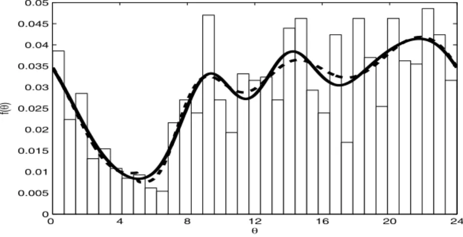
In this section we consider a data set of crimes perpetrated in Chicago on May 11th 2007, obtained from www.chicagocrime.org. Figure 5 gives the 24 hour clock times of the 1240 crimes committed on this day.
For this data set we fitted the most general algorithm with the circular uniform distribution plus up to 5 SSB distribution components and also considered models with a uniform component and SSB terms with a common origin. The optimal model according to the DIC3 criterion was the fixed origin model with 4 SSB components (DIC3 = 4575) whereas the optimal full model contains five SSB components with DIC3 = 4582. Figure 4.1 shows the fits of the optimal full model (solid line) and the optimal, common origin model (dashed line).
0:00
12:00
18:00 + 6:00
Figure 5: Perpetrated times of crimes on may 11th at Chicago
0 4 8 12 16 20 24 0 0.005 0.01 0.015 0.02 0.025 0.03 0.035 0.04 0.045 0.05 θ f( θ )
5
Conclusions and extensions
In this article, we have developed a new, semi-parametric model for circular data which appears to compare favourably with the well known, von Mises mixture model. A number of extensions are possible.
Firstly, we have here used the BIC as a classical model choice criterion. It would also be possible to consider other criteria such as the Akaike (1974) information criterion (AIC). Our practical experience shows that the use of the AIC generally leads to overfitting for the Bernstein polynomial models and that the SSB mixture models still perform better than both the von Mises mixture and Bernstein polynomial models under this criterion. Al-ternative criteria such as the corrected AIC could also be considered. Also from a Bayesian viewpoint, alternative model selection criteria such as those proposed by Celeux et al (2006) could be considered. In practice, we have found that the models selected using these criteria are usually the same as for DIC3 used here.
Secondly, we have considered Bayesian inference for a mixture of a uni-form density and various SSB distributions of fixed size. It is also possible to consider the simple SSB mixture model without the assumption that a uniform component is always present. In practice, this seems to introduce little advantage as in the great majority of data sets we have examined, a uniform component is virtually always fitted. Furthermore, this introduces some extra technical restrictions in the setting up of the MCMC algorithm due to the necessity of maintaining the identifiability of the fitted model.
Thirdly, it is straightforward to implement Bayesian inference for SSB mixtures of random dimension via reversible jump (Green 1995, Richardson and Green 1997) or birth-death (Stephens 2000) MCMC techniques. One advantage of this approach is that this avoids jumps in the predictive density due to the fact that this is mixed over the parameter distribution.
Fourthly, it would be interesting to examine the possible increase in ef-ficiency from using a mixture of SSB distributions with continuous beta pa-rameters instead of restricting the papa-rameters to be integers. Finally, from a Bayesian standpoint, instead of using a finite mixture of SSB distribu-tions, we might consider using continuous, Dirichlet process mixtures of SSB distributions, along the lines of Kottas (2006).
References
[1] Akaike, H. (1974). A new look at the statistical model identification.
IEEE Transactions on Automatic Control, 19, 716–723.
[2] Babu, G.J., Canty, A.J. and Chaubey, Y.P. (2002). Application of Bern-stein polynomials for smooth estimation of a distribution and density function. Journal of Statistical Planning and Inference, 105, 377–392. [3] Celeux, G., Forbes, F., Robert, C. and Titterington, M. (2006) Deviance
Information Criteria for missing data models.Bayesian analysis,1, 651– 674.
[4] Cox, D.R. and Lewis, P.A.W. (1966). The Statistical Analysis of Series of Events. Methuen: London.
[5] Dempster, A.P., Laird, N.M. and Rubin, D.B. (1977). Maximum likeli-hood from incomplete data via the EM algorithm. Journal of the Royal Statistical Society Series B, 39, 1–38.
[6] Evans, M., Hastings, N. and Peacock, B. (2000). von Mises Distribution. In Statistical Distributions, 3rd ed., Wiley: New York, pp. 189–191. [7] Fern´andez-Dur´an, J.J. (2004). Circular distributions based on
nonnega-tive trigonometric sums. Biometrics, 60, 499–503.
[8] Ferreira, J.T.A.S., Juarez, M.A. and Steel, M.F.J. (2005). Directional Log-spline Distributions.Working Paper,05-17, Centre for Research in Statistical Methodology, Warwick University.
[9] Green, P.J. (1995). Reversible jump Markov chain Monte Carlo compu-tation and Bayesian model determination. Biometrika,82, 711–732. [10] Jammalamadaka, S.R. and Kozubowski T.J. (2003). A new family of
circular models: The wrapped Laplace distributions, Advances and Ap-plications in Statistics 3(1), 77-103, 2003.
[11] Kakizawa, Y. (2004). Bernstein polynomial probability density estima-tion. Journal of Nonparametric Statistics,16, 709–729.
[12] Kottas, A. (2006). Dirichlet process mixtures of beta distributions, with applications to density and intensity estimation. UCSC Department of Applied Math and Statistics Technical Reports, ams2006-12.
[13] Fisher, N.I. (1989). Smoothing a sample of circular data. Journal of Structural Geology, 11, 775–778.
[14] Mardia, K.V. and Jupp, P. E. (1999). Directional Statistics, Wiley: Chichester.
[15] McLachlan, G. and Peel, (2000). Finite Mixture Models. Wiley: New York.
[16] Mooney A., Helms P.J. and Jolliffe I.T. (2003). Fitting mixtures of von Mises distributions: a case study involving sudden infant death syn-drome. Computational Statistics and Data Analysis, 41, 505–513. [17] Petrone, S. (1999a). Random Bernstein polynomials.Scandinavian
Jour-nal of Statistics, 26, 373–393.
[18] Petrone, S. (1999b). Bayesian density estimation using random Bern-stein polynomials. Canadian Journal of Statistics, 27, 105–126.
[19] Petrone, S. and Wassermann, L. (2002). Consistency of Bernstein poly-nomial posteriors. Journal of the Royal Statistical Society Series B,64, 79–100.
[20] Richardson, S. and Green, P. (1997). On Bayesian analysis of mixtures with an unknown number of components (with discussion). Journal of the Royal Statistical Society Series B,59, 731–792.
[21] Robert, C. P. y Rousseau, J. (2003) A mixture approach to bayesian goodness of fit. Technical report, 2002-9, Universit Paris Dauphine. [22] Schwarz, G. (1978). Estimating the dimension of a model. Annals of
Statistics, 6, 461–464.
[23] Speigelhalter, D.J., Best, N.G., Carlin, B.P. and van der Linde, A. (2002). Bayesian measures of model complexity and fit (with discus-sion), Journal of the Royal Statistical Society Series B, 64, 583–616.
[24] Stephens, M.A. (1969). Techniques for directional data. Technical Re-port,150, Department of Statistics, Stanford University.
[25] Stephens, M. (2000). Bayesian analysis of mixture models with an un-known number of components – an alternative to reversible jump meth-ods. Annals of Statistics, 28, 40–74.
[26] Vitale, R.A. (1975). A Bernstein polynomial approach to density esti-mation. InStatistical inference and related topics (ed. Madan Lal Puri), Vol 2, 87–100. Academic Press, New York.
Appendix: Proofs of theorems
Proof of Theorem 1First note that ifθ ∼ SSB(0, α, β) then
E[cos(pθ)] = E[cos(2πpX)] where X ∼ B(α, β) = " 1 0 cos(2πpx) 1 B(α, β)x α−1(1−x)β−1dx = 1 B(α, β) " 1 0 cos(2πpx) β−1 j=0 β−1 j xα−1+jdx assuming β ∈IN = 1 B(α, β) β+j−1 j=0 (−1)j β−1 j Ip(α+j −1) where Ip(C) = " 1 0
cos(2πpx)xCdx and similarly,
E[sin(pθ)] = E[sin(2πpX)] = 1 B(α, β) β+j−1 j=0 (−1)j β−1 j Jp(α+j−1) where Jp(C) = " 1 0 sin(2πpx)xCdx Also
E[cos(pθ)] = E[cos(2πp(1−Y))] where Y ∼ B(β, α) = E[cos(2πpY)] = 1 B(α, β) α+j−1 j=0 (−1)j α−1 j Ip(β+j−1) E[sin(pθ)] = E[sin(2πp(1−Y))]
= −E[sin(2πpY)] = 1 B(α, β) α+j−1 j=0 (−1)j+1 α−1 j Jp(β+j−1).
Now observe that
Ip(0) = " 1 0 cos(2πpx)dx= 0 Jp(0) = " 1 0 sin(2πpx)dx= 0 Ip(1) = " 1 0 xcos(2πpx)dx= 1 2πp[xsin(2πpx)] 1 0− 1 2πp " 1 0 sin(2πpx)dx= 0 Jp(1) = " 1 0 x sin(2πpx)dx=− 1 2πp[xcos(2πpx)] 1 0+ 1 2πp " 1 0 cos(2πpx)dx=− 1 2πp Now consider Ip(C). For C≥2,
Ip(C) = " 1 0 x Ccos(2πpx)dx = 1 2πp xCsin(2πpx)1 0− C 2πp " 1 0 x C−1sin(2πpx)dx = − C 2πp " 1 0 x C−1sin(2πpx)dx = C (2πp)2 xC−1cos(2πpx)1 0− C(C−1) (2πp)2 " 1 0 x C−2cos(2πpx)dx = C (2πp)2 − C(C−1) (2πp)2 Ip(C−2) (7) and thereforeIp(2) = 2
(2πp)2 andIp(3) = (2πp3)2 which satisfy the formula given
in Theorem 1. Assume now that the formula is valid for c= 2, . . . , C. Then
Ip(C+ 2) = C+ 2 (2πp)2 − (C+ 2)(C+ 1) (2πp)2 Ip(C) from (7) = C+ 2 (2πp)2 − C 2 c=1 (−1)c−1 C! (C−2c+ 1)! 1
(2πp)2c from the induction assumption
= C+ 2 (2πp)2 + C 2 c=1 (−1)c+1−1 (C+ 2)! (C+ 2−2(c+ 1) + 1)! 1 (2πp)2(c+1)
= C+ 2 (2πp)2 + C+2 2 c=2 (−1)c−1 (C+ 2)! (C+ 2−2c+ 1)! 1 (2πp)2c = C+2 2 c=1 (−1)c−1 (C+ 2)! (C+ 2−2c+ 1)! 1 (2πp)2c
which demonstrates the formula for Ip(C). Equally, we have the recurrence relation
Jp(C) =−21
πp −
C(C−1)
(2πp)2 Jp(C−2) (8)
which implies that Jp(2) =− 1
2πp andJp(3) =− 1 2πp +
3!
(2πp)3 which satisfy the
formula of Theorem 1. Assuming the formula is valid for c= 2, . . . , C then
Jp(C+ 2) = −21 πp − (C+ 2)(C+ 1) (2πp)2 Jp(C) from (8) = − 1 2πp − (C+ 2)(C+ 1) (2πp)2 C+12 c=1 (−1)c C! (C−2c+ 2)! 1 (2πp)2c−1
from the induction assumption = − 1 2πp − C+1 2 c=1 (C+ 2)! (C−2c+ 2)! 1 (2πp)2c+1 = C+2+1 2 c=1 (−1)c (C+ 2)! (C+ 2−2c+ 2)! 1 (2πp)2c−1
which demonstrates the formula for Jp(C) and proves the theorem. ‡
Proof of Corollary 1
Letθ ∼ SSB(ν, α, β). Then:
E[cos(pθ)] = E[cos(mod(pν +pθ0,2π))] whereθ0 ∼ SSB(0, α, β) = E[cos(pν +pθ0)]
= cospνE[cospθ0]−sinpνE[sinpθ0]
= 1 B(α, β) ⎧ ⎨ ⎩ β−1 j=0 (−1)j β−1 j (cos(pν)Ip(α+j −1)−sin(pν)Jp(α+j −1)) ⎫ ⎬ ⎭.
The other expressions can be derived similarly by using the expansions of sin(A+B) and cos(A +B) and the fact that if X ∼ B(α, β), then Y =