Johns Hopkins University, Dept. of Biostatistics Working Papers
11-7-2006
PENALIZED LIKELIHOOD AND BAYESIAN
METHODS FOR SPARSE CONTINGENCY
TABLES: AN ANALYSIS OF ALTERNATIVE
SPLICING IN FULL-LENGTH cDNA
LIBRARIES
Corinne Dahinden
Seminar fur Statistik
Giovanni Parmigiani
The Sydney Kimmel Comprehensive Cancer Center, Johns Hopkins University & Department of Biostatistics, Johns Hopkins Bloomberg School of Public Health, [email protected]
Mark C. Emerick
Department of Physiology, Johns Hopkins School of Medicine
Peter Buhlmann
Seminar fur Statistik
This working paper is hosted by The Berkeley Electronic Press (bepress) and may not be commercially reproduced without the permission of the copyright holder.
Suggested Citation
Dahinden, Corinne; Parmigiani, Giovanni; Emerick, Mark C.; and Buhlmann, Peter, "PENALIZED LIKELIHOOD AND BAYESIAN METHODS FOR SPARSE CONTINGENCY TABLES: AN ANALYSIS OF ALTERNATIVE SPLICING IN FULL-LENGTH cDNA LIBRARIES" (November 2006).Johns Hopkins University, Dept. of Biostatistics Working Papers.Working Paper 123. http://biostats.bepress.com/jhubiostat/paper123
Penalized Likelihood and Bayesian Methods for Sparse
Contingency Tables: An Analysis of Alternative Splicing
in Full-Length cDNA Libraries
Corinne Dahinden
Seminar f¨
ur Statistik
ETH Z¨
urich
CH-8092 Z¨
urich, Switzerland
email:
[email protected]
Giovanni Parmigiani
Departments of Oncology and Biostatistics,
Johns Hopkins Schools of Medicine and Public Health
Baltimore, MD
email:
[email protected]
Mark C. Emerick
Department of Physiology,
Johns Hopkins School of Medicine
Baltimore, MD
email:
[email protected]
Peter B¨
uhlmann
Seminar f¨
ur Statistik
ETH Z¨
urich
CH-8092 Z¨
urich, Switzerland
email:
[email protected]
Summary. We develop methods to perform model selection and parameter estimation in log-linear models for the analysis of sparse contingency tables to study the interaction of two or more factors. Typically, datasets arising from so-called full-length cDNA libraries, in the context of alternatively spliced genes, lead to such sparse contingency tables. Maximum Likelihood estimation of log-linear model coefficients fails to work because of zero cell entries. Therefore new methods are required to estimate the coefficients and to perform model selection. Our suggestions include computationally efficient `1- penalization (Lasso-type) approaches as well as Bayesian methods using MCMC. We compare these procedures in a simulation study and we apply the proposed methods to full-length cDNA libraries, yielding valuable insight into the biological process of alternative splicing.
Keywords: Graphical models, Hierarchical models, Interactions, Lasso, Log-linear models,
1
Introduction
One of the most striking discoveries of the genomic era is the unexpectedly small number of genes in the human genome. This number has decreased from more than 100000 (Liang et al.,
2000) through 30000-35000 (Int. Consortium, 2001; Ewing and Green, 2000; Venter et al.,
2001) and is now estimated to be roughly between 20000 and 25000 (Int. Consortium, 2004;
Southan, 2004), tens of thousands less than initially expected and essentially the same number as found in phenotypically much simpler organisms. Thus, a question of overriding biological significance is, how complex phenotypes of higher organisms arise from limited genomes. Part of the explanation may be that many genes undergo a process called alternative RNA splicing, which can generate many distinct proteins from a single gene.
RNA splicing is a post-transcriptional process that occurs prior to mRNA translation. After the gene has been transcribed into a pre-messenger RNA (pre-mRNA), it consists of intronic regions destined to be removed during pre-mRNA processing (RNA splicing), as well as exonic sequences that are retained within the mature mRNA. Occurring after transcription is the actual splicing process, during which it is decided which exons are retained in the mature message and which are targets for removal. This is modeled as a non-deterministic process where exons and introns are retained and deleted in different combinations to create a diverse array of mRNAs from a common coding sequence. This process is known as alternative RNA splicing. Mapping of large numbers of expressed sequence tags (ESTs) onto genomic DNA has revealed that many genes are alternatively spliced. Depending on the source, the percentage lies between 35% and 60% (Mironovet al.,1999;Brettet al.,2000;Int. Consortium,2001;Brettet al.,2002;Carninci et al., 2005; Zavolan, van Nimwegen, and Gaasterland, 2003; Imanishi et al., 2004). However, the information which can be derived from ESTs as far as alternative splicing is concerned is limited for various reasons. One of these is transcript end bias resulting from the fact that ESTs are prevalently derived from sequencing the ends of cDNAs. And as ESTs are short in length (typically around 300-500bp), only a portion of the cDNA can be covered. This means that splice sites in the middle region of the gene are strongly underrepresented in EST libraries and therefore hard to detect by these means. One way to overcome this difficulty is by screening many full-length cDNAs. By recording the complete cDNA from a mature RNA for the same gene again and again, a full-length cDNA library, also known as single-gene library (SGL), builds up and detailed information about how specific exon combinations go together becomes available. The functional regions of the proteins are grouped in domains which in many cases correspond to a single exon which encodes these domains. For example a transcription factor consists of a DNA binding domain and a regulatory domain. Thus the alteration of the exon structure corresponds to an alteration in the function of this particular domain. The central premise is that correlated expressions of domains point to a functional association. If domains interact functionally then their splicing should be co-regulated. It is further believed that such interaction patterns are regulated in a tissue and development specific way.
As more investigators become interested in this type of information, and large-scale single-gene libraries become available, there is a strong need for reliable statistical methods for analyzing the resulting datasets. Due to the large number of potential combinations in highly alternatively spliced genes, any library will only comprise a small portion of the total theoretically possible
inventory of combinations. Statistically, this leads us to deal with sparse contingency tables in which dimensions represent exons and cells represent variants. Investigating interactions among exons in the formation of a message requires addressing a model selection problem that is challenging both inferentially and computationally.
Here, within the context of log-linear models, we develop different statistical methods to analyse sparse contingency tables, such as e.g. those arising from single-gene libraries. These methods are compared in a simulation study and then applied to full-length cDNA datasets. As far as these are concerned, the main focus lies in identifying the interaction structure, estimating the interaction strength, and assessing how the interaction structure varies over different tissues or stages of development in a single tissue. The analysis of these interaction patterns is a first step towards understanding the underlying regulatory program.
Section 2 is an introduction to contingency tables and log-linear models. In Section 3, we describe different frequentist and Bayesian model selection procedures for log-linear models. Detailed algorithms and implementations of these are given in Section 4. The summary of a simulation study is given in Section 5, and the proposed methods are applied to real single-gene libraries in Section6. Sections2and3are presented in general terms, as the methodology developed there can be applied to a broad spectrum of problems.
2
Contingency Tables and Log-linear Models
2.1
General Methodology
In this section we provide general definitions and notations.
A contingency table is formed by classifying a number of objects according to a setCof criteria which correspond to categorical variables. The classified objects can be represented as the cell counts of a so-called |C|-way contingency table, where |C| represents the number of elements inC. If we adopt the notation of Dellaportas and Forster(1999), which goes back to Darroch, Lauritzen, and Speed (1980), the table is the set I = Q
c∈CIc, where Ic is the set of levels of
the factor c. An individual cell is denoted by i = (ic, c ∈ C) and the corresponding cell count
byni. The total number of cells in the table is m=|I|= Q
c∈C|Ic|.
A natural way of representing the distribution of the cell counts is via a vector of probabilities
p = (pi, i ∈ I). If a total number of n individuals is observed and the objects are classified
independently, then the distribution of the corresponding cell counts n = (n1, n2, . . . , nm)t is
multinomial with probability p. A general log-linear model represents p as log (p) = Xβ, where β is a vector of unknown regression coefficients. The choice of the design matrix X
will be discussed below. A specific parametrization of the log-linear model is in terms of the ”u parameters”, introduced by Birch (1963), see for example Bishop, Fienberg, and Holland
(1975). The resulting model is called a log-linear interaction model: logpi =
X
a⊆C
ua(ia) (i∈I), (1)
where ia is the marginal cell ia= (iγ, γ ∈a), indicating the levels of a subseta of C. Thus the
In matrix formulation, this corresponds to a matrix X= [Xa, a⊆C], where X∅ is a column of
1’s (intercept) and Xc1 ∈R
m×|Ic1| forc
1 ∈C is an incidence matrix where each row has a unit entry in the column of the level to which it belongs;Xc1c2 :=Xc1 :Xc2 is defined by taking each
column of Xc1 and multiplying it element-wise by each column of Xc2; Xc1c2c3 = Xc1 : (Xc2 : Xc3); and this can be generalized to any number of factors a={c1, . . . , cl} ⊆C.
The model (1) and the corresponding matrix X are highly overparametrized. To ensure iden-tifiability, we impose sum-to-zero constraints on ua:
X
i∈I
iγ=const
ua(ia) = 0 ∀a⊆C,∀γ ⊂a,∀iγ ∈Iγ, (2)
whileu∅ is a normalizing constant ensuring that all cell probabilities add up to 1. Equation (1)
in vector formulation becomes
log(p) = X
a⊆C
Ua. (3)
One can prove that under the constraints (2) it holds that Ua⊥Ub for a 6= b, i.e. P
i∈Iua(ia)ub(ib) = 0 (see Lemma1in the Appendix A for details). In matrix formulation, the
constraints (2) impose constraints on the sub-matrices Xa of X (a ⊆C) in the representation
log (p) =Xβ: XbtXa= 0 for a 6=b. If we reparametrizeXa by choosing orthonormal columns,
it holds that Xa is an orthonormal basis of span(Ua): Xa has dimensionality R|I|×da, where
da = Q
γ∈a(|Iγ| −1). Imposing the constraints (2) on the design matrixX corresponds in terms
of ANOVA to choosing a poly-contrast. The log-linear interaction model (1) or (3) with the constraints (2), takes on the following form in matrix formulation:
log (p) = Xβ. (4)
The correspondence to (3) holds by using Ua = Xaβa, where βa is the part of the vector β
corresponding to the interaction term a. In case of factors with only 2 levels, βa is a scalar,
otherwise it is a vector of dimension da. If one assumes a smaller model without some of the
interaction terms, the model takes on the same form (4) with some columns removed from the design matrix X.
2.2
Contingency Tables and Log-Linear Models for Binary Factors
Translating the formalism above to binary factors, the domain of our problem, is straightfor-ward. The set C = {1, . . . , D} of criteria corresponds in our case to D factors with 2 levels 1/-1. These represent the D exons, which are either retained or deleted. The set I is the whole array of 2D theoretically possible exon combinations. A single cell i of the contingency table can therefore be represented by a D-dimensional binary vector (i1, . . . , iD), with each ij
indicating whether the corresponding exon is present or absent. The corresponding log-linear interaction model (1) with the constraints (2) can be written in the following way:
logpi =β∅+ X l∈{1,...,D} βlil+ X i,k j<k∈{1,...,D} βjkijik+. . .+β12...Di1i2· · ·iD.
From this representation, one can straightforwardly derive the design matrix X and the para-metrization (4).
The formulation above corresponds to the situation where we have D cassette exons. Cassette exons are segments of the DNA which are either spliced in or spliced out. We note here that the term exon throughout this work represents either a complete exon or an exon segment, as alternative splicing at times occurs within exon boundaries, resulting in inclusion of exon fragments in the mature transcript. The situation corresponds to D factors with two levels (spliced in or spliced out). The methodology in Section 2.1 is held very general so that it can also be applied to problems with more than two levels per factor. For example in the context of single-gene library analysis, if two exons are mutually exclusive, an appropriate representation for the pair is given by using a single factor with 3 levels.
3
Model Selection
In this section we introduce different model selection strategies in log-linear models. In Section
3.2 we develop first an `1-regularization model selection approach, which is then expanded to the new so-called level-`1-regularization approach in Section 3.3. We favor the latter over the former; see also the results of the simulation study in Section 5. In Sections 3.4 and 3.5, Bayesian model selection strategies are introduced.
3.1
Non-Hierarchical Versus Hierarchical Models
Hierarchical models are a subclass of models such that if an interaction term βa is zero, than
all higher order interaction terms βb for b ⊇ a are also zero. While it is possible that the
true underlying interaction model may not be hierarchical from a biological standpoint, a difficulty in the use of non-hierarchical models arises from the fact that they are not invariant under reparametrization. We have chosen the design matrix X with sum-to-zero constraints on ua (see (2)) to ensure identifiability, and we used a specific, namely an orthonormal basis
of span(Ua). In terms of ANOVA, this choice is equivalent to choosing a poly-contrast. We
could have imposed different constraints or have chosen a different basis of span(Ua), and this
would have resulted in a different design matrix X or in terms of ANOVA, a different choice of contrast. Suppose we have found an interaction vector β for one parametrization of the log-linear model and that this vector corresponds to a non-hierarchical model, meaning there is at least one lower order interaction termβa equal to zero, whileβb 6= 0 for at least oneb ⊇a.
If we reparametrize the model, using a different design matrix, the coefficient for the model terma may not be zero anymore. On the other hand, by reparametrizing a hierarchical model, all zero terms remain zero after reparametrization. Therefore, hierarchicity is preserved after reparametrization while non-hierarchicity depends on the parametrization. This is a distinct advantage of working within the hierarchical class. In a hierarchical model, all zero coefficients can directly be interpreted in terms of conditional independence, while for non-hierarchical models, the zero terms of the hierarchized model (βa = 0 with βb = 0 ∀b ⊇ a) feature this
with the according parametrization.
3.2
`
1-Regularized Model Selection
The Lasso, originally proposed byTibshirani (1996) for linear regression, performs regularized parameter estimation and variable selection at the same time. It is defined as follows:
b βλ = arg min β " X i (Y−Xβ)2i +λX i |βi| # ,
where Y = (Y1, . . . , Yn) is the response vector. It can also be viewed as a penalized Maximum
Likelihood estimator, as P
i(Y−Xβ)
2
i is proportional to the negative log-likelihood function
for Gaussian linear regression. While the MLE for the general regression model is no longer uniquely defined and very poor in the case of more variables than observations, the Lasso estimator is still reasonable forλ >0. For our analysis, we have a similar problem, namely that the MLE is not defined in case of zero counts in the contingency table: a detailed description of the existence of the MLE in general log-linear interaction models is given in Christensen
(1991). Inspired by the Lasso, we estimate our parameter vectorβby the following expression:
b βλ = arg min β " −l(β) +λ m X j=1 |βj| # , (5)
where l(β) is the log-likelihood function l(β) = logPβ[n] ∝ Pjnj(Xβ)j. This minimization
has to be calculated under the additional constraint that the cell probabilities add to 1:
m X
j=1
exp{(Xβ)j}= 1. (6)
The problem of the optimization (5) is that the solution is no longer independent of the choice of the orthogonal subspaces Xa. That is, if any set of orthogonal columns Xa of X
is reparametrized by a different orthogonal set, we get a different solution. To avoid this un-desirable outcome we use a penalty that is intermediate between the `1- and the `2-penalties. This penalty, called group-`1-penalty, has the following form:
X a⊆C kβak`2, where kβak 2 `2 = X j (βa)2j
It has been proposed by Yuan and Lin (2006) for the linear regression problem with factor variables. The estimator of β then becomes
b βλ = arg min β −l(β) +λX a⊆C a6=∅ kβak`2 , (7)
subject to the constraint in (6). By imposing a penalty function on the coefficients of the log-linear interaction terms, overfitting as it might occur by using MLE is prevented. Furthermore, the `1-penalty encourages sparse solutions as far as the single components ofβ are concerned, the group `1-penalty encourages sparsity at the interaction level, meaning that the vector βa,
which corresponds to the interaction termais either present or absent in the model as a whole. In case of factors with only 2 levels, the group `1-penalty and the `1-penalty are equivalent. For both the `1-, and the group `1-regularization, the parameter λ can be assessed e.g. by 10-fold cross-validation: we divide the individual counts into ten equal parts and in turn leave out one part for the rest (90%) to form a training contingency table with cell counts ntrain.
The solution for an array of values for λ, the so-called solution path, is calculated according to an algorithm described in Section 4.1. The corresponding vectors of cell probabilities are denoted by pβb
λ
. We then use the remaining 10% of the cell counts ntest to calculate the
predictive negative log-likelihood score −Pm j=1ntest,j·log pj(βb λ ) Pm j=1ntest,j , (8)
which is proportional to the out-of-sample negative log-likelihood. This score is on the same scale when varying the number of observations and may therefore be used to compare contin-gency tables of the same dimension but with different numbers of cell entries. The parameter λ is chosen as the value which minimizes the cross-validated score in (8).
The resulting model does not necessarily have to be hierarchical and if we consider the hierar-chical model induced by this procedure, it might happen that the final model is large, e.g. if a single high order interaction is estimated to be active. Therefore we set up a regularization approach which we calllevel-`1-regularized model selection to prevent the algorithm to choose single high-order interaction.
3.3
Level-
`
1-Regularized Model Selection
The algorithm fits models as described above for each level of possible interaction order. This means, a model is fitted with main effects only, and the predictive negative log-likelihood score (8) is calculated for the best main effects model (level 1). The same is done for the model including all main effects and first order interactions (level 2). Proceeding accordingly, we get |C|log-likelihood scores corresponding to the|C| levels. Finally, the model with minimal score (8) among all levels is chosen.
With this procedure we tend to select smaller models which can be better hierarchized and interpreted in terms of conditional independence in contrast to the ordinary`1-model selection procedure.
3.4
Non-Hierarchical Bayesian Model Selection
The Bayesian approach we choose is most closely related to what was proposed by
1994. We use a Markov chain Monte Carlo algorithm based on Stochastic Search Variable Selection (SSVS): SSVS is a procedure proposed by George and McCulloch (1993) to perform variable selection in the standard linear regression model. We adapt this procedure to log-linear models. But instead of assuming a normal mixture model for the coefficients of interest as in SSVS, we follow an approach proposed by Geweke (1994), and assume the coefficients to be a mixture of a point mass at zero and a normal distribution. The complete model is described as follows:
n∼M ultinom(p) with log(p) = Xβ,
βa|γa∼(1−γa)I0+γaN(0, σ2a1da) independent for all a⊆C,
γa∼Ber(prγa) independent for alla⊆C,
σ2
a ∼Γ
−1(l, u) independent for all a⊆C,
(9)
where I0 is a point mass at zero and γa is a Bernoulli variable with probability parameterprγa reflecting prior belief that the corresponding interaction term Ua is present. The parameters
σ2
a follow an inverse gamma distribution with parameters l and u. In our simulation study,
we also considered fixed values for σ2
a. The choice of the prior parameter l, u and prγa is discussed in Section 4.2. In the absence of strong prior belief, it is reasonable to assume that allσ2
a are identically distributed. By imposing prior distributions on the log-linear parameters
βa, it would be possible to incorporate further prior knowledge in the form of existence of
correlation or signs of correlation between the different criteria C. One way is to use a prior with expectation different from zero for the corresponding log-linear term (E[βa|γa = 1]6= 0).
See for exampleDellaportas and Forster(1999) for a more detailed discussion on normal priors for the log-linear parameters βα.
We introduce variables αa, whereαa∼ N(0, σa21da) and we set βa=αa if γa= 1 and βa= 0 if
γa = 0 independent of the value ofαa: βa=αaγahas then the desired distribution in (9). This
construction is mentioned, but not implemented, in Geweke (1994).
The calculation of the posterior distribution f(γ,α,σ2|n) is now required. This cannot be done directly and Monte Carlo approximations are needed, for example from Gibbs sampling. We first calculate the univariate conditional distributions of the parameters αa or components
of αa if it is a vector:
f(αa|n,γ,α\a,σ2)∝f(n|γ,α)f(αa|σa2)∝exp{n·(X∅α∅+Xaαaγa)}f(αa|σa2).
Although this univariate conditional density is not of any recognized form, we can prove that it is log-concave (see Lemma 2in the Appendix A for details) and therefore sampling from it can be efficiently done using adaptive rejection sampling, as proposed by Gilks and Wild (1992). Sampling σ2
a is straightforward, as
f(σa2|n,γ,α,σ2\a) =f(σ2a|αa)∝f(αa|σ2a)f(σ
2
a), (10)
and we can easily show that σa2|αa∼Γ−1(α2a/2 +l, u+ 1/2). Therefore we can sample σ2a from
an inverse gamma distribution. In the case where σ2
a is assumed to be fixed, this sampling step
can be omitted. To sample from f(γa|n,γ\a,α,σ2), we compute the conditional Bayes factor
BF in favour of γa= 1 versus γa = 0. The conditional posterior distribution of γa is Bernoulli
with pγa =
BF
1+BF. Thus we can sample
The Bayes factorBF is given by
BF = f(n|γa= 1,γ\a,α)prγa f(n|γa= 0,γ\a,α)(1−prγa)
.
The parameters αa, σ2a and γa are updated in turn for all a ⊆ C. In this way we are able
to efficiently sample from the full posterior f(α,γ,σ2|n) and derive from it the posterior of f(β,γ,σ2|n). From the marginal posterior distribution f(γ|n), we can estimate the model probabilities by the sample proportions for γ, with the most promising models corresponding to the most frequently observed γ. From f(β|n, γ) we can derive the distribution for the interaction strength vector β conditional on the modelγ.
3.5
Hierarchical Bayesian Model Selection
We adapt the algorithm described above in a way that allows only moves from one hierarchical model to another, so that we never leave the class of hierarchical models. A hierarchical model is determined by its generators, that is the maximal terms a ⊆ C which are present in the model. The only individual model term which may be removed from a hierarchical model so that it remains hierarchical is a generating term. In addition, Edwards and Havranek (1985) define the dual generators, which are the minimal terms that are not present in the model. The only individual model terms which may be added to the model so that it remains hierarchical are the dual generators.
We consider all hierarchical models to be equally likely and denote the set of generators and dual generators of a hierarchical model corresponding to γ with Gγ. We use a Metropolis Hastings
algorithm to sample from the full posterior distributionf(γ,α,σ2|n). We propose a move from one model γt to the next model γt+1 by choosing an element G
γt. Thus we randomly sample an element a ∈ Gγt and the corresponding γa is set to one or zero respectively. The resulting
γ is denoted asγt+1. The corresponding move is accepted with acceptance probability:
min 1,f(n|γ t+1,αt)|G γt| f(n|γt,αt)|G γt+1| .
The sampling procedure for αa and σa2 is performed exactly as in the non-hierarchical case
described in Section 3.4.
4
Implementation
4.1
Algorithm for
`
1-Regularization for Factors With Two Levels
For the regularization approaches we calculate βb λ
over a large number of values of λ in order to do some cross-validation using (8). For this purpose, an efficient algorithm is required. As one can easily verify by introducing Lagrange multipliers, finding the solution to (7) under the
constraint (6) is equivalent to minimizing an unconstrained function g(β): g(β) = −l(β) +n m X j=1 exp (µj) +λ X a⊆C a6=∅ kβak`2, (11)
with µ = Xβ. Here, g is a convex function. If each factor has two levels only, as in our application with single-gene libraries, we can set up an algorithm, which efficiently yields the estimates for a whole sequence of parameters λ. Let A denote the set of active interaction terms, which means for a ∈ A it holds that βa 6= 0; XA is the corresponding sub-matrix of
X,βA the corresponding sub-vector ofβ andgA isg restricted to the subspaceβA. We restrict
ourselves to the currently active set A, where∇gA and ∇2gA are well-defined:
∇gA(βA, λ) = −XtA{n−n·exp (XAβA)}+λ(0, sign(βA))t
∇2g
A(βA, λ) = n·XtAdiag{exp (Xβ)}XA.
The algorithm, which is an adaption of the path following algorithm proposed byRosset(2005), is set up as follows:
(1) Start with βb = (−log (m),0, . . . ,0)
(2) Set: λ0 = maxj∈C j6=∅ |(Xtn) j|=n,A={∅}and t = 0. (3) While (λt > λmin) (3.1) λt+1=λt− (3.2) A=A ∪ {j /∈ A:|[Xt·n−n·expXβb ]j|> λt+1} (3.3) βb is updated as βbt+1 =βbt− ∇2gA(βbt, λt+1) −1 · ∇gA(βbt, λt+1). (3.4) A=A \ {j ∈ A:|βbt+1,j|< δ} (3.5) t=t+ 1
The pairs (βbt, λt), obtained from the algorithm above, represent the estimates from (7) under
the constraint (6) for a range of penalty parametersλte.g. (t=,2, . . .). The choice of the step
length represents the tradeoff between computational complexity and accuracy. To increase accuracy, one can perform more than one Newton step (3.3) if the gradient starts deviating from zero. The coefficient δ is also flexible. Typically it is chosen in the order of. The lowest λ for which one wants the solution to be calculated is denoted by λmin.
4.2
Prior Specification for Bayesian Methods
For the Bayesian estimation of the parameter vector, we must specify the parameters for the prior distribution of σ2
a: σ2a plays a role that is similar to that of the parameter λ in the
Lasso. The lower σ2
a, the smaller the estimated coefficient βba. An empirical Bayes approach
to the implementation could be to specify this parameter by cross-validation. While feasible for the`1-regularization approaches above, cross-validation becomes prohibitive for the MCMC approaches because of the computational demands. Dellaportas and Forster (1999) proposed a fixed value of two for all a in C, e.g. σa2 = σ2. Placing a normal prior with mean zero and variance two on each αa means that with probability 0.95, each of these effects will increase
or decrease the ratio of any two cell probabilities by a factor of no more than 10. This is a relatively vague prior, and can be appropriate when no prior information is available. However, our simulation study will illustrate that the final results can be highly sensitive to the choice of this value. To mitigate this sensitivity, we assumeσ2 to have an inverse gamma distribution with mean and variance equal to one, as described in Section 3.4.
In addition, for non-hierarchical model selection, we have to specify the prior distribution for γa. We set γa ∼ Ber(prγa), where prγa reflects prior belief that the corresponding interaction term Ua is present. Without prior knowledge, we assume here that all possible models are a
priori equally likely, corresponding to prγa = 1/2 for all a⊆C.
This prior is especially attractive when coupled with MAP estimation, as done here, because it effectively cancels out of the MAP calculation. In other situations, this prior may be less compelling. For example, it may be of interest to report posterior probabilities of properties of sets in the model space, such as marginal posteriors of the inclusion of certain coefficients or marginal posteriors of the presence of high order interactions. Then one has to evaluate carefully the mass that priors give to those sets, and one might have to reconsider the choice of the prior distributions to get reasonable posterior probabilities of these sets. In addition, asD, the number of exons, increases, estimating the MAP in the model space becomes difficult and marginal posteriors of summaries such as the model size or the maximum order of interaction may be all that can be reliably estimated. In those circumstances, we suggest graphing these posteriors along with the corresponding priors probabilities, and/or to report Bayes factors.
5
Simulation Study
5.1
Data
We choose the true underlying interaction vector β consisting of 5 factors of 2 levels. By enumerating the factors from 1 to 5, the generators of the model are 345 + 235 + 234 + 135 + 123 + 14, which means that all third and fourth order interactions are absent, only five of ten second order interactions and all first order interactions are present. This defines γ and the corresponding coefficients of β are independently simulated using a normal distribution with mean zero and variance one.
Then, 250 draws from a multinomial distribution with probability vectorpwhere log (p) =Xβ, are taken. This corresponds to a reasonable number of cDNA in a single-gene library. This
is then repeated 10 times, independently of each other. With our choice of β, the resulting contingency tables are sparse. With the simulated cell counts, βb is estimated with different
methods described in the previous sections and these methods are then compared in various ways described in the next Section 5.2.
5.2
Criteria
For the MCMC approaches, the maximum a posteriori (MAP) estimators are used. As a model selection score (MSS), the fraction of correctly assigned model terms is reported:
MSS = 1 m m X j=1 |1{βj6=0}−1{βbj6=0}|.
Moreover, we consider the root mean squared error for the interaction coefficients,
RM SE = v u u t 1 m m X j=1 (βbj −βj)2.
For assessing how much the estimation ofβ varies over multiple datasets, we calculate for every coefficientβbj the estimated standard deviation
b
σj. The means of these standard deviations are
reported as V ar= 1 m m X j=1 b σj, a measure of variability.
To compare the different procedures for estimation of probabilitiesp = exp (Xβ), we simulate a new datasetnnew of 4000 observations and calculate the out-of-sample negative log-likelihood
score (NLS) similar to the score in (8): N LS(βb) =− m X j=1 nnew,j·log n pj(βb) o
5.3
Results
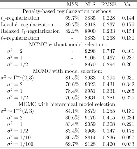
The results are summarized in Table 1. We notice that the penalty-based regularization proaches proposed in this article leads to comparable or better results than the Bayesian ap-proaches with respect to the NLS-score, RMSE and the variation (Var).
The level- and the relaxed`1-regularization are both competitive and can be better than MCMC for model selection.
The results of the MCMC procedures are sensitive to the choice of the prior value or the prior distribution for σ2. A flat prior for α
a (σ2 = 2) results in worse estimations than with a prior
Table 1: Comparison of different methods to estimate the interaction strength vector β. MSS, NLS, RMSE and Var are described in Section 5.2. The additional methods relaxed `1-regularization and `2-regularization listed in the Table are explained in Section 5.3.
MSS NLS RMSE Var Penalty-based regularization methods:
`1-regularization 69.7% 8835 0.228 0.144 Level-`1-regularization 89.7% 8918 0.237 0.179 Relaxed `1-regularization 82.2% 8900 0.233 0.154 `2-regularization - 8833 0.238 0.130
MCMC without model selection:
σ2 = 2 - 9296 0.747 0.401 σ2 = 1 - 9105 0.467 0.287 σ2 = 1/2 - 8970 0.294 0.201
MCMC with model selection:
σ2 ∼Γ−1(2,3) 81.5% 8933 0.294 0.231 σ2 = 2 76.6% 9023 0.431 0.342 σ2 = 1 78.4% 8951 0.331 0.265 σ2 = 1/2 76.6% 8934 0.281 0.225
MCMC with hierarchical model selection:
σ2 ∼Γ−1(2,3) 84.1% 8879 0.255 0.180 σ2 = 2 80.6% 9176 0.415 0.284 σ2 = 1 83.4% 9059 0.308 0.221 σ2 = 1/2 83.4% 8966 0.247 0.178 σ2 = 1/10 86.3% 8814 0.236 0.097 σ2 = 1/100 69.7% 9128 0.420 0.033
this prior hyperparameter may be difficult in practice, while we can easily optimize λ in the regularization approach by cross-validation.
The MCMC approaches without model selection perform poorly, as should be expected from data generated by a sparse model. MCMC methods based on a non-hierarchical model selection are also clearly inferior to the hierarchical counterpart. This is not surprising, as we have simulated data from a hierarchical model.
In Table 1 we have also added an additional approach, denoted by `2, the equivalent to the `1-regularization but instead of an `1-penalty, using an `2-penalty on the coefficients of the log-linear model. This method is equivalent to the MAP estimator with Gaussian priors onβa
in (9), with the parameter of the distribution optimized by cross-validation. This Ridge-type method does not perform variable selection, but it is very competitive for all other criteria that we assessed.
parameter λ, the idea of this method is to control variable selection and parameter estimation by incorporating two penalty parameters. For linear regression it has been proven theoretically as well as empirically (Meinshausen, 2005) that relaxed `1-regularization is often better than Lasso. Details can be found in the Appendix C.
Overall, the level-`1-regularization has good model selection performance in combination with low negative log-likelihood score (NLS) and a low mean squared error for the trueβ (RMSE). In addition, it is feasible to optimize the tuning parameter λ by cross-validation as the com-putational cost is very low compared to the MCMC approaches. On the other hand, posterior distributions of estimates from MCMC methods provide additional information about uncer-tainty in the model space, compared to point estimates from `1− or `2− regularization.
6
Real Data from Single-Gene Libraries
6.1
Dataset
We estimate the splicing interaction pattern for a dataset corresponding to the itpr1 gene, one of three mammalian genes encoding receptors for the second messenger inositol 1,4,5-trisphosphate (InsP3). This gene is subject to alternative RNA splicing, with seven sites of transcript variation, 6 of these within the ORF and among these, D = 5 were completely assessed in the single-gene libraries. Five single-gene libraries were built, one for adult rat cerebrum as well as four for different stages of postnatal cerebellar development, namely on days 6, 12, 22 and 90, the latter being considered as adult. Each library consists of between 179 and 277 transcripts which were assessed, i.e. Pm
j=1nj ∈[179,277]. This gene is 89% identical
at the cDNA level and 95% identical at the amino acid level with the human receptor gene. The complete dataset can be found in Regan et al.(2005).
6.2
Results
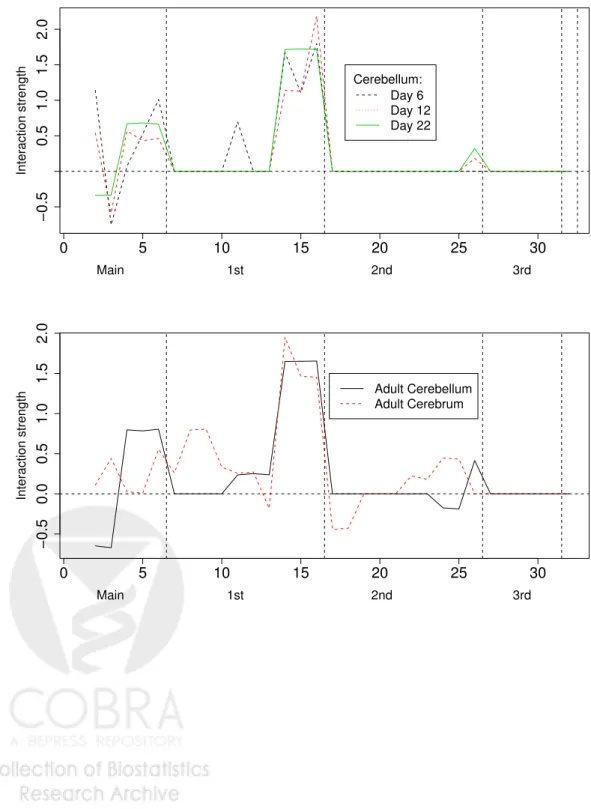
Unless stated differently, we report the results using the level `1-penalization method. We display the interaction vector βb graphically by plotting the components βbj for the different
tissue and development stages in Figure 1. We clearly see that the exons interact mainly in pairs and there is no estimated higher order interaction in the splicing interaction pattern of rat cerebellum. We further notice that the main interaction pattern is very well conserved over different developmental stages. A strong mutual interaction between the exons number three, four and five can be observed in all development stages of rat cerebellum as well as in the cerebral tissue. The biggest changes in the interaction pattern during development of rat cerebellum occur from postnatal day six to day 12. This can be seen at position number 10 on the x-axis in Figure 1, and it corresponds to the first order interaction between exons two and three, and from day 12 to day 16, the first main effect changes in sign and magnitude. The first main effect decreases progressively from day 6 to adult, reversing in sign between day 12 and 22. Between day 22 and 90, the interaction pattern is strongly conserved. Comparing the splicing interaction patterns between cerebellum and cerebrum in the adult rat, we see a
much more complex pattern in the cerebrum, involving several second order interactions, and therefore a clear distinction from that of the cerebellum.
A natural way of visualizing a log-linear model is in terms of a graph. A graph G = (V,E) consists of a finite set V of vertices and a finite set E of edges between these vertices. In our context, the vertices correspond to the different alternatively spliced exons. We form the so-calledindependence graph by connecting all pairs of vertices that appear in the same generator. From this graph we can directly read off all marginal and conditional independences by the global Markov property for undirected graphs which states: if two sets of variables a and b are separated by a third set of variables c then a and b are conditionally independent given c (a⊥⊥b|c), where for three subsets a, b and cof V, we saycseparates a and b if all paths from a tob intersect c.
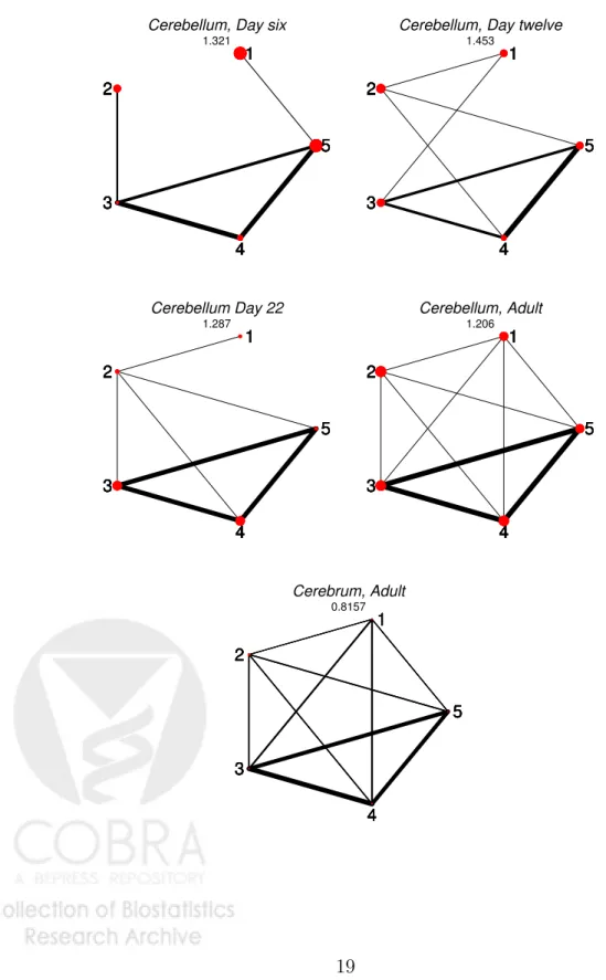
The independence graphs for the estimated log-linear models are drawn in Figure 2, where the thickness of the edges are proportional to the largest corresponding coefficient of the interaction vectorβb and the radius of the vertices are chosen proportional to the corresponding main effect
coefficient. Figure 2 graphically exploits the strongly conserved interactions between exons three, four and five. Except for a rather strong interaction between exon two and three on day six, all other interactions appear to be rather small. The graphical representation of the interaction pattern of adult rat cerebrum reveals a more complex interaction pattern with no conditional independences.
We have also estimatedβwith the hierarchical Bayesian approach using MCMC. For the choice ofσ2 = 1 this resulted in very similar interaction patterns as for the level`
1-penalization method (see Figure 3). For σ2 = 2 it led to remarkably different results. Details can be found in the Supplementary Material. In addition to this, a further dataset was analyzed where the details can be found in the Supplementary Material as well.
As mentioned in Section4.2, we report Bayes Factors in favour of certain model sizes to get an idea of which order the models are. For rat cerebellum day six, these Bayes factors are 0 for the main effects model, 1.92 for first order interaction, 18.29 for second, 93.95 for third and 0 for fourth order interaction. Similarly for the other developmental stages, it is always the third order interaction model with the largest Bayes Factor. Interestingly, the MAP in the model space is a model involving only second order interactions, but the Bayes Factors speak in favour of a third order interaction model.
7
Conclusions
We have developed efficient frequentist and Bayesian methods for identifying interaction pat-terns in single-gene libraries. In a simulation study, the results of the new level-`1-regularization method are superior to hierarchical Bayesian approaches and other frequentist regularization methods. With real data, the level`1-regularization and hierarchical Bayesian approach led to similar results, subject to a specific choice of priors for the Bayesian method. Massive compu-tational advantages are on the side of the level-`1-method: the algorithm is sufficiently efficient such that cross-validation becomes feasible which in turn allows for an objective choice of the tuning parameter. On the other hand, posterior distributions of estimates from the hierarchical
Bayes approach can provide a measure of uncertainty on the model or models selected that is harder to derive in a penalized likelihood setting.
The approaches and results presented here can provide valuable insight into the underlying processes in alternative splicing in general, and specifically in the brain development experi-ments considered here. Most striking is the strong conservation over developmental stages at day 12, 22 and 90 (adult); some differences are showing between postnatal day six and day 12. Also, the conservation between the cerebellum and cerebrum is less pronounced than over developmental stages. Finally, second- or higher-order interaction terms seem to be of minor relevance, suggesting that in this gene/tissue combination, direct interaction mainly happens between pairs of exons, but not combinations of three or more exons.
The level-`1-method is not restricted to analyzing alternative splicing data, but is a much more general tool which can be applied to a wide variety of problems involving sparse contingency ta-bles. An R package will be made available soon for download under http://stat.ethz.ch/~dahinden/R/loglin.html.
Figure 1: The upper panel shows the estimated splicing interaction vectors βb of rat cerebellum
tissues at postnatal days six, 12 and 22. The lower panel shows the splicing interaction vectorβb
of rat cerebellum tissues at the age of 90 days as well as the splicing interaction vectorβb of rat
cerebral tissue at the age of 90 days. Within an interaction degree, the sequence of coefficients is ordered from left to right as follows: e.g. for 2nd order interactions, 123,124,125, . . . ,345, where 1, . . . ,5 represent exons 12, 23B, 40, 41, and 42 in the rip3r1 gene, as described inRegan
et al. (2005). 0 5 10 15 20 25 30 −0.5 0.0 0.5 1.0 1.5 Main 1st 2nd 3rd Interaction strength Day 6 Day 12 Day 22 Cerebellum: 0 5 10 15 20 25 30 −0.5 0.0 0.5 1.0 1.5 Main 1st 2nd 3rd Interaction strength Adult Cerebellum Adult Cerebrum
Figure 2: Independence graphs for the estimated log-linear models for the itpr1 gene. For each graph, the predictive probability score (8) is reported as a goodness of fit measure. Note the strong mutual interaction between exons three, four and five.
Cerebellum, Day six 1.321 1 2 3 4 5 1 2 3 4 5 1 2 3 4 5 1 2 3 4 5 1 2 3 4 5
Cerebellum, Day twelve 1.453 1 2 3 4 5 1 2 3 4 5 1 2 3 4 5 1 2 3 4 5 1 2 3 4 5 Cerebellum Day 22 1.287 1 2 3 4 5 1 2 3 4 5 1 2 3 4 5 1 2 3 4 5 1 2 3 4 5 Cerebellum, Adult 1.206 1 2 3 4 5 1 2 3 4 5 1 2 3 4 5 1 2 3 4 5 1 2 3 4 5 Cerebrum, Adult 0.8157 1 2 3 4 5 1 2 3 4 5 1 2 3 4 5 1 2 3 4 5 1 2 3 4 5
Figure 3: Interaction vectorsβbfor the gene itpr1 estimated by the hierarchical MCMC estimator
with σ2a = 1 for all a. Note the close similarity between this interaction pattern and the one from the level-`1-regularization estimator in Figure 1.
0 5 10 15 20 25 30 −0.5 0.5 1.0 1.5 2.0 Main 1st 2nd 3rd Interaction strength Day 6 Day 12 Day 22 Cerebellum: 0 5 10 15 20 25 30 −0.5 0.0 0.5 1.0 1.5 2.0 Main 1st 2nd 3rd Interaction strength Adult Cerebellum Adult Cerebrum
Appendix A Lemma 1. Ua⊥Ub for a 6=b, i.e. Pi∈Iua(ia)ub(ib) = 0.
Proof. Fora∩b=∅it holds that
X i ua(ia)ub(ib) = X ia X i,with ia=const ua(ia)ub(ib) = X ia ua(ia) X i,with ia=const ub(ib) = X ia ua(ia) 1 |ia| X i ub(ib) = 0, because X i ub(ib) = 0,
while |ia| is the total number of different marginal cells ia. For a∩b =γ it holds that X i ua(ia)ub(ib) = X iγ X ib,with ib∩γ=iγ X i,with ib=const ua(ia)ub(ib) = X iγ X ib,with ib∩γ=iγ ub(ib) X i,with ib=const ua(ia) = X iγ X ib,with ib∩γ=iγ ub(ib) 1 |ib\γ| X i,with iγ=const ua(ia) = 0 because of (2) .
Lemma 2. The function f(αa|n,γ,α\a) is log-concave for the prior distributions chosen as
described in (9).
Proof. Without loss of generality we assume that αa is univariate. The proof for the case that
αa is a vector is exactly the same but for a single component of αa. We have to prove that the
function h(αa) is concave for
h(αa) = nα∅+ntXaαaγa−
1 2σ2α
2
a,
where α∅ is the normalizing constant ensuring that all cell probabilities add up to 1. This
constant depends on αa. As the last two terms are concave it remains to be shown that
nα∅(αa) is concave. For γa = 0 this term is constant and h(αa) is therefore concave. For
γa = 1, we setX0 =X\∅ and α0 =α\∅, it then holds
h(αa) = nα∅ =−nlog m X i=1 exp{(X0α0)i}, h0(αa) = −n Xt aexp (X 0 α0) Pm i=1exp}(X 0 α0) i} , h00(αa) = −n (X2 a)texp (X 0 α0)Pm i=1exp{(X 0 α0)i} − {Xatexp (X 0 α0)}2 [Pm i=1exp{(X 0 α0) i} 2 ] ,
where exp (X0α0) has to be understood as the componentwise application of the exponential function and likewise for X2
a. We now have to show that h
00(α
a) is less than zero. If we denote
exp (X0α0) by u and Xa with x, it is sufficient to prove that m X j=1 x2juj m X i=1 ui−(xtu)2 ≥0.
The above expression is
X i,j j<j ((x2jujui+x2iuiuj)−(2xiuixjuj)) = X i,j j<j (x2j +x2i −2xixj)uiuj = X i,j,i<j (xj −xi)2uiuj,
which is greater than zero, as u>0. This proves Lemma2.
Appendix B
We note that ifβ is a minimum of g, thenβA is a minimum of gA.
In our application with single-gene libraries, all factors have two levels only, which allows to construct an efficient algorithm. Since the gradient
∇ " −l(β) +n m X j=1 exp (µj) # =−Xt· {n−n·exp (Xβ)},
where exp(Xβ) is understood as the componentwise exponential function, it follows that for a minimum βA of gA, the following equation holds:
∇gA(βA) =−XtA· {n−n·exp (XAβ)}+{0, sign(βA)}t·λ= 0 (12)
Without loss of generality, we can restrict ourselves to the subspace β ∈R−×
Rm−1, because the constraint (6) can only be satisfied for β∅ < 0 as is proved in the following Lemma 3.
Therefore β∅ ∈ A.
Lemma 3. β∅ <0 for a minimum of g(β) for all λ∈R+.
Proof.
log (p) =Xβ<0 which yields (1, . . . ,1)Xβ=mβ0 <0 this impliesβ∅ <0.
This holds because (1, . . . ,1) is orthogonal to all columns of X except for the first one. Additionally for β being a minimum, a necessary condition is:
|[Xt· {n−n·exp (Xβ)}]j|< λ,∀j /∈ A. (13)
Conditions (12) and (13) are sufficient for β being a minimum of (11). To find the β’s that solve these equations for an array of values forλ, we set up a so-called path following algorithm.
The idea is to start from an optimal solution βλ0 for λ
0, and follow the path for decreasing λ, using a second-order approximation for βA. In the following, we restrict ourselves to the currently active set A, omitting the indexA. It then holds:
∇g(βt+1, λt+1) = 0≈ ∇g(βt, λt+1) +∇2g(βt, λt+1)δβ. This implies (14) δβ = −∇2g(βt, λt+1)−1∇g(βt, λt+1).
The algorithm tries to follow the optimal path as close as possible. At each step, it aims to meet the conditions (12) and (13). In step (3.2), the active set A is identified, which forces
b
β to meet the condition (13). In step (3.3), a Newton step as described in (14) is performed. Starting from a solution which meets condition (12), the new βb
λ
approximately meets (12) again
Appendix C
Relaxed `1-Regularized Model Selection
The two-stage relaxed Lasso is defined as follows:
b βλ,µ= arg min β " −l(βM λ) +µ X j∈Mλ |βj| # , where Mλ ={1 ≤ k ≤ m|βbkλ 6= 0}, βb λ as in (7) and βM
λ denotes a vector consisting only of components in Mλ.
For selecting the parametersλ and µ, a similar approach is chosen as with `1-regularization in Section 3.2. First, we compute all possible submodels Mλ for the full dataset. Then, for each
submodel the second parameter µis selected as for the regular `1-regularization by computing the negative log predictive probability score (8). Finally, the parameters (λ, µ) are chosen to minimize the score (8). When we prefer hierarchical over non-hierarchical models, we consider a hierarchical Mλ, meaning that λ and µ are assessed using the hierarchical model induced
by Mλ, i.e. the smallest hierarchical model which contains all elements of Mλ. Due to the
second-stage penalization, βb λ,µ
is not necessarily hierarchical though.
Supplementary Material
Under http://stat.ethz.ch/~dahinden/Biometrics/Suppmat.pdf the supplementary ma-terial containing results from additional datasets as well as results for additional variable selec-tion strategies can be viewed.
Acknowledgements
Dahinden’s research was partially founded by the Swiss National Science Foundation (SNF). Parmigiani was partly supported by NSF grant DMS034211.
References
Aitchison, J. (1986), The Statistical Analysis of Compositional Data, Chapman and Hall, Lon-don.
Birch, N.W. (1963), Maximum Likelihood in Three-Way Contingency Tables, Journal of the Royal Statistical Society, Ser. B, 25, 220–233.
Bishop, Y., Fienberg, S., and Holland, P. (1975), Discrete Multivariate Analysis, MIT Press, Cambridge, Massachusetts and London, UK.
Brett, D., Hanke, J., Lehmann, G., Haase, S., Delbruck, S., Krueger, S. R., and J. Bork, P. (2000), EST Comparison Indicates 38% of Human mRNAs Contain Possible Alternative Splice Forms, FEBS Letters 474, 83–86.
Brett, D., Pospisil, H., Valcarcel, J., Reich, J., and Bork, P. (2002), Alternative Splicing and Genome complexity, Nature Genetics 30, 29–30.
Christensen, R. (1991),Linear Models for Multivariate Time Series, and Spatial Data, Springer-Verlag.
Darroch, J.N., Lauritzen, S.L., and Speed, T.P. (1980), Markov Fields and Log-Lineaer Inter-action Models for Contingency Tables, Annals of Statistics 8, 522–539.
Dellaportas, P. and Forster, J. (1999), Markov Chain Monte Carlo Model Determination for Hierarchical and Graphical Log-Linear Models, Biometrika 86, 615–633.
Edwards, D. and Havranek, T. (1985), A Fast Procedure for Model Search in Multidimensional Contingency Tables, Biometrika 72, 339–351.
Emerick, M.C., Stein, R., Kunze, R., McNulty, M., Regan, M.R., Hanck, D.L., and Agnew, W.S. (2006), Profiling the Array of Cav3.1 Variants From the Human T-Type Calcium Channel
Gene CACNA1G: Alternative Structures, Developmental Expression and Biophysical Varia-tions. Proteins: Structure, Function and Bioinformatics .
Ewing, B. and Green, P. (2000), Analysis of Expressed Sequence Tags Indicates 35000 Human Genes, Nature Genetics 25, 232–234.
FANTOM Consortium, RIKEN Genome Exploration Research Group, and the Genome Science Group (Genome Network Project Core Group) (2005) The Transcriptional Landscape of the Mammalian Genome, Science 309, 1559–1563.
George, E. I. and McCulloch, R.E. (1993), Variable Selection via Gibbs Sampling, Journal of the American Statistical Association 88, 881–889.
Geweke, J. (1996), Variable Selection and Model Comparison in Regression, inBayesian Statis-tics 5, edited by J. M. Bernardo, J. O. Berger, A. P. Dawid and A. F. M. Smith, University Press, Oxford, 609–620.
Gilks, W.R. and Wild, P. (1992), Adaptive Rejection Sampling for Gibbs Sampling, Applied Statistics 41, 545–557.
Imanishi, T., Itoh, T., Suzuki, Y., O’Donovan, C., Fukuchi, S., Koyanagi, KO, Barrero, RA., Tamura, T., Yamaguchi-Kabata, Y., and Tanino, M. (2004), Integrative Annotation of 21037 Human Genes Validated by Full-Length cDNA Clones, PloS Biology 2, 1–20.
International Human Genome Sequencing Consortium (2001), Initial Sequencing and Analysis of the Human Genome, Nature 409, 860–921.
International Human Genome Sequencing Consortium (2004), Finishing the Euchromatic Se-quence of the Human Genome, Nature 431, 931–945.
King, R. and Brooks, S.P. (2001), Prior Induction in Log-Linear Models for General Contin-gency Table Analysis, Annals of Statistics 29, 715–747.
Liang, F., Holt, I., Pertea, G., Karamycheva, S., Salzberg, S., and Quackenbush, J. (2000), Gene Index Analysis of the Human Genome Estimates Approximately 120000 Genes, Nature Genetics 25, 239–240.
Madigan, D. and York, J.C. (1997), Bayesian Methods for Estimation of the Size of a Closed Population. Biometrika 84, 19–31.
Meinshausen, N. (2005), Lasso with Relaxation, Technical Report 129, ETH Z¨urich .
Mironov, A.A., Fickett, J.W., and Gelfand, M.S. (1999), Frequent Alternative Splicing of Hu-man Genes, Genome Research 9, 1288–1293.
Ntzoufras, I., Forster, J., and Dellaportas, P. (2000), Stochastic Search Variable Selection for Log-linear Models, Journal of Statistical Computation and Simulation 68, 23–37.
Regan, M.R., Lin, D.D.M., Emerick, M.C., and Agnew, W.S. (2005), The Effect of Higher Order RNA Processes on Changing Patterns of Protein Domain Selection: A Developmen-tally Regulated Transcriptome of Type 1 Inositol 1,4,5-Trisphosphate, Proteins: Structure, Function and Bioinformatics 59, 312–331.
Rosset, S. (2005), Following Curved Regularized Optimization Solution Paths, in Advances in Neural Information Processing Systems 17, edited by L. K. Saul, Y. Weiss, and L. Bottou, MIT Press, Cambridge, 1153–1160.
Southan, C. (2004), Has the yo-yo Stopped? An Assessment of Human Protein-Coding Gene Number, Proteomics 4, 1712–1726.
Tibshirani, R. (1996), Regression Shrinkage and Selection via the Lasso, Journal of the Royal Statistical Society, Ser. B, 58, 267–288.
Venter, J., Adams, MD., Myers, EW., Li, PW., and Mural, RJ. et al. (2001), The Sequence of the Human Genome, Science 291, 1304–1351.
Yuan, M. and Lin, Y. (2006), Model Selection and Estimation in Regression with Grouped Variables, Journal of the Royal Statistical Society, Ser. B, 68(1), 49–67.
Zavolan, M., van Nimwegen, E., and Gaasterland, T. (2003), Splice Variation in Mouse Full-Length cDNAs Identified by Mapping to the Mouse Genome, Genome Research 12, 1377– 1385.