ISSN 1392 – 124X INFORMATION TECHNOLOGY AND CONTROL, 2009, Vol. 38, No. 1
PARAMETER IDENTIFICATION
FOR ASYMMETRICAL POLYNOMIAL LOSS FUNCTION
Piotr Kulczycki *
**, Aleksander Mazgaj **
* Polish Academy of Sciences, Systems Research Instituteul. Newelska 6, PL-01-447 Warsaw, Poland e-mail: [email protected]
** Cracow University of Technology, Department of Automatic Control ul. Warszawska 24, PL-31-155 Cracow, Poland
Abstract. The parameter identification for problems where losses arising from overestimation and underestimation
are different and can be described by an asymmetrical and polynomial function is investigated in this paper. The Bayes decision rule allowing to minimize potential losses is used. Calculation algorithms are based on the nonparametric methodology of statistical kernel estimators, which releases the method from dependence on distribution type. Three basic cases are considered in detail: a linear, a quadratic, and finally a general concept for a higher degree polynomial – here the cube-case is described in detail as an example. For each of them, the final result constitutes a numerical proce-dure enabling to effectively calculate the optimal value of a parameter in question, presented in its complete form which demands neither detailed knowledge of the theoretical aspects nor laborious research of the user. Although the above method was investigated from the point of view of automatic control problems, it is universal in character and can be applied to a wide range of tasks, also outside the realm of engineering.
Keywords: parameter identification, Bayes estimation, asymmetrical polynomial loss function, nonparametric
es-timation, kernel estimators, numerical algorithm.
1. Introduction
The dynamic development of computer science and metrological technology now means obtaining more and more precise measurements, as well as col-lecting received information with the aim of further processing forever more complex control algorithms. However, more precise and faster instrumentation only manage to lessen the error in measurements, not eliminate it entirely. As an example: one of the main parameters of mechanical systems – mass, is often not measured at all, or only grossly assumed on the basis of general conditioning. Moreover, it often changes with consumption of fuel or other substances used in the production process.
Quality of control is influenced not only by errors in measurement but also the structure of the model itself, which directly determines the range of possibi-lities for the reflection of properties in real processes. A full consideration of all phenomena occurring in an object is not just impossible, but even pointless, as the complexity of such a model would make it unusable. Thus, it is not achievable to accurately measure para-meters occurring in a model, not only due to metrolo-gical limitations, but also because of structural rea-sons, where many parameters represent a wide range
of phenomena, and so, often do not possess “exact” values. For further details in this topic see [3, 4, 17-19, 21], where subject literature can also be found, which in the case of identification is particularly diverse re-garding wealth of methodology as well as the variety of tasks it is applied to.
As identification is in practice always subject to a higher goal (usually conditioned by the control algo-rithm), very valuable results can be obtained thanks to the consideration – during estimation of the parame-ters’ values – of the losses implied through errors, as mentioned earlier, unchecked in practice. In control engineering applications such losses can often be de-scribed by the function assuming the following asymmetrical and polynomial form:
⎪⎩ ⎪ ⎨ ⎧
≥ λ − λ λ
− λ
≤ λ − λ λ
− λ − = λ λ
0 ˆ for ) ˆ (
0 ˆ for ) ˆ ( ) 1 ( ) , ˆ
( k kk
b a
l , (1)
resul-ting from modeling errors, and complexity, and in consequence usefulness of the approach proposed.
Similar conditioning can also be shown for many problems outside the area of automatic control, or even broadly understood engineering. For example, as stated by Kahneman – a Nobel laureate in the field of economics – behavior in business is not completely ra-tional. According to his theory, a human reacts strong-ly to extreme stimuli and is disposed to exaggerating losses as well as undervaluing gains. This fear of large losses enables animals to survive in nature, however, in the economy it leads to an illogical dread of change. Therefore, if one describes the psychological prefe-rences of the ordinary person, then it can be defined by formula (1), for example with k=2, i.e. in the quadratic case. Here an inverse relationship to losses and gains is represented by nonsymmetry, and fear of extremes by quadratic form.
Consider therefore the typical situation where one has m values of the investigated parameter x1,
2, ... , m
x x obtained directly by measuring or with the aid of auxiliary quantities. In this paper, the uncer-tainty of the examined parameter is considered with a probabilistic approach. For identification of character-istics of probabilistic measure the statistical kernel estimators methodology [8, 20, 22] will be used. This is the current leading concept of nonparametric esti-mation, the present development of which is con-nected with a dynamic growth of possibilities and in particular the universal availability of computer sys-tems. As opposed to classical parametric estimation, where firstly one arbitrarily assumes a typical prob-ability distribution type, and next calculates the values of its parameters, in the case of kernel estimators prac-tically no assumptions are made, and atypical, com-plex and multimodal distributions can be treated ex-actly the same as simple, even textbook cases. Finally, a Bayes estimator, optimal in the sense of minimiza-tion of expectaminimiza-tion value of losses, will be found ac-cording to principles of the Bayes decision rule [2].
Three basic cases will be investigated in the fol-lowing: linear (Section 3.1), quadratic (Section 3.2), and higher degree polynomial (Section 3.3) – here the cube-case will be described in detail. In every case, the final result will be a procedure for the calculation of values for an optimal estimator. Thanks to the pres-ence of complete established algorithms applied here, as well as clear analytical forms of quantities used, its practical implementation will consist of only routine introduction dependencies. The proposed procedure is universal and can be applied in a wide range of tasks, not only in the field of engineering. Furthermore, the method worked out can be used for other uncertainty approaches apart from that of probability, e.g. fuzzy logic [7].
The preliminary version of this article was presen-ted as the conference-paper [15]. Its main theses have also been included in the synopses [10-12].
List of Notations In order of appearance:
l – loss function
λ – parameter ˆ
λ – estimator of the parameter λ
k – degree of asymmetrical polynomial loss func-tion
a – coefficient of the asymmetrical polynomial loss function regarding underestimation
b – coefficient of the asymmetrical polynomial loss function regarding overestimation
N – set of natural numbers
1
x, x2, ... ,xm – random sample, interpreted here as the measurements of the estimated parameter m – size of random sample
R – set of real numbers
Z – set of states of nature
D – set of possible decisions
f – density of probability distribution
z – state of nature
d – decision B
l – Bayes loss function
B
d – Bayes decision
X – random variable ˆ
f – kernel estimator of density of probability distri-bution
x – independent variable, interpreted here as esti-mated parameter
i, j – natural indices
K – kernel
h – smoothing parameter
r – degree of the plug-in method ˆ
σ – estimator of standard deviation
10
ψ , ψs, g1, g2, g3, g, p, P, R, L – auxiliary parameters and functions used in the plug-in method
1
s , s2, ... ,sm – modifying parameters
c – intensity of modifying procedure
s – auxiliary parameter used for modifying proce-dure
M – mass submitted to control
t – time
1
X – first coordinate of state of a dynamic system
2
X – second coordinate of state of a dynamic system
U – control
t-o
J – minimum-time performance index for optimal control
U
T – time to reach the origin when the control U is used
ˆ
M – estimator of the parameter M ˆ
I – primitive function of the kernel K
y – auxiliary variable
i
U , Vi, Wi – auxiliary functions used in the
investi-gated algorithm
L – auxiliary function for Newton’s algorithm q
J – quadratic performance index for optimal control
Q, R – matrices of losses of the quadratic
per-formance index
X – state vector of a dynamic system U – control vector
Λ – parameter ˆ
Λ – estimator of the parameter Λ )
, (μ σ
N – normal distribution with the expectation value μ and the standard deviation σ
2. Mathematical Preliminaries 2.1. Bayes Decision Rule
The main aim of decision theory [2] is the selec-tion of a concrete decision based only on a repre-sentation of measure characterizing the imprecision of states of nature. Let there be given a nonempty set of states of nature Z = R, and a nonempty set of possible decisions D⊂R. Assume that the imprecision of states of nature is of probability type and its distribu-tion is described by the density f : R→[0, )∞ . Let there be given also the loss function l:D×Z→R, while its values l d z( , ) can be interpreted as losses occurring in a hypothetical case, when the state of nature is z and the decision d is taken. If for every
d∈D the integral
Rl d z f z( , ) ( ) dz
∫
exists, then the Bayes loss function l DB: → ∪ ± ∞R { } can be defined asR
( ) ( , ) ( ) d
B
l d =
∫
l d z f z z . (2)Every element dB∈D such that l dB( )B = min ( )B
d D∈ l d
is called a Bayes decision, and the above procedure – a Bayes decision rule. As the above definition shows, the Bayes decision dB is chosen from the elements of
the set of possible decisions so as to minimize the value of the Bayes loss function – from the probabilis-tic point of view: the expectation value of losses after the decision d was made. Further details can be found in the book [2].
2.2. Statistical Kernel Estimators
Let the one-dimensional random variable X,with a distribution having the density f , be given. Its kernel estimator f :R→[0,∞) is calculated on the basis of the m-element simple random sample x1, x2, ... ,xm
acquired experimentally from the variable X, and is defined in its basic form by the formula
1
1
ˆ ( ) m i
i
x x
f x K
mh = h
−
⎛ ⎞
= ⎜ ⎟
⎝ ⎠
∑
, (3)where the function K :R→[0,∞), which is measur-able, symmetrical relative to zero, and has a weak global maximum at this point, fulfilling the condition
RK x( ) dx=1
∫
, and is called a kernel, whereas the positive coefficient h is known as a smoothing pa-rameter [8, 20, 22].Fixing values introduced in definition (3), i.e. choosing the form of the kernel K and calculating the smoothing parameter h value, is most often carried out using the mean square criterion.
Thus, from the statistical point of view, the form of the kernel seems not to have essential meaning, thanks to which it becomes possible for the choice of the function K to be arbitrary, taking into account above all required properties of the estimator obtained, e.g. class of regularity, positive values, or other qualities important in the case of a particular problem, especial-ly the convenience of calculations.
As opposed to the form of the kernel, the value of the smoothing parameter h has significant influence on the quality of the estimator obtained. In any case, convenient algorithms have been developed in order to calculate this value on the basis of a random sample. For the one-dimensional case considered here, the most convenient is the so-called plug-in method. Its concept consists of the calculation of this parameter using an approximate method, and after r steps im-proving the result, one obtains a value close to opti-mal. In practice, it is taken that r≥2, with the lowest possible value recommended. On the basis of simu-lation research carried out for the needs of the task worked out in this paper, r=3 was assumed. In this case the plug-in method consists of the application of the following formulas:
10 1 2 11
945 ˆ 64π ψ
σ
−
= , (4)
while ˆσ denotes the estimator of a standard deviation
2 2
1 1
1 1
ˆ ( )
1 ( 1)
m m
i i
i i
σ x x
m = m m =
= −
−
∑
−∑
(5)and
1 11 (8) 1
10
2 (0)
( )
L g
mP L ψ
⎛− ⎞
= ⎜ ⎟
⎝ ⎠ (6)
1 9 (6) 2
8 1
2 (0)
( ) ( )
L g
mP L ψ g
⎛ − ⎞
= ⎜ ⎟
⎝ ⎠ (7)
1 7 (4)
3
6 2
2 (0)
( ) ( )
L g
mP L ψ g
⎛ − ⎞
= ⎜ ⎟
finally
1 5
2 4 3
( )
( ) ( )
R K h
mP K ψ g
⎛ ⎞
= ⎜ ⎟
⎝ ⎠ , (9)
where the finite quantities are defined as
2
R
( ) ( ) d
R K =
∫
K x x (10)2
R
( ) ( ) d
P K =
∫
x K x x (11)( ) 2 1
1 1
1
( ) m m p i j
p p
i j
x x
ψ g L
g m g +
= =
−
⎛ ⎞
= ⎜ ⎟
⎝ ⎠
∑∑
for p=1, 2,... . (12) The kernel K, applied in estimator (3), is used only in the last step. In all other steps, the different kernel L, more convenient for the plug-in method, may be used. The value of the smoothing parameter h introduced in definition (3) is the same for all kernels, mapped to particular elements of the random sample. In “dense” areas of such elements, the above value should be lessened (which allows for better showing of specific features of the distribution), as opposed to areas where such elements are “sparse” and it should be increased (which causes additional smoothing of “tails”). The parameter modification procedure achieves this goal in compliance with the following algorithm:
(A) the kernel estimator fˆ is specified according to basic formula (3);
(B) the modifying parameters si >0 of the form ˆ ( ) c
i i
f x s
s
−
⎛ ⎞
= ⎜⎜ ⎟⎟
⎝ ⎠ for i=1, 2, ... , m , (13)
are calculated, while the nonnegative parameter c shows the intensity of the modification proce-dure, whereas s is the geometric mean of the numbers f xˆ ( )1 , f xˆ( ), ..., ( )2 f xˆ m ;
(C) the kernel estimator with the modification of the smoothing parameter, is ultimately defined as
1
1 1
ˆ ( ) m i
i i i
x x
f x K
mh = s hs
⎛ − ⎞
= ⎜ ⎟
⎝ ⎠
∑
. (14)Note that taking c=0 results in si ≡1 and conse-quently basic form (3).
Details of the above-presented methodology of sta-tistical kernel estimators can be found in the books [8, 20, 22].
3. The Algorithm 3.1. Linear Case
As an example illustrating the investigations pre-sented in this section, an optimal control [1] problem
will be considered. The control performance index, which exists here, can also refer to quality of identi-fication allowing the creation of an optimal procedure for estimation of object parameter values, thereby no-tably lowering excess sensitivity of such systems to the inaccuracy of modeling.
Thus, consider the following dynamic system:
1 1
2 2
0 ( ) 0 1 ( )
( ) 1 ( ) 0 0 ( )
X t X t
U t X t
X t
M
⎡ ⎤
⎡ ⎤ ⎡ ⎤⎡ ⎤ ⎢ ⎥
= +
⎢ ⎥ ⎢ ⎥⎢ ⎥ ⎢ ⎥
⎣ ⎦ ⎣ ⎦
⎣ ⎦ ⎢⎣ ⎥⎦ , (15)
where the positive parameter M represents a mass submitted to a force according to Newton’s second law of dynamics [1 – Section 7.2]. Then X1, X2 and
U denote position and velocity of the mass, and the force regarded here as a control, respectively. Con-sider the time-optimal control task, the basic form of which consists of bringing the system’s state to the origin, in minimal and finite time, assuming the con-trol values are bounded. Thus, the performance index
t-o
J is given here as
t-o( ) U
J U =T , (16)
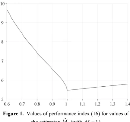
where TU denotes the time to reach the origin when the control U is used, assumed as infinity if the origin is not reached at all with this control. For details see the classic textbook [1 – Chapter 7]. Fundamental meaning for phenomena existing in the control system lies in the proper identification of value of the parame-ter M. The control is defined in relation to the value of the estimator ˆM, actually different from the value of the parameter M in the object. A detailed analysis can be found in the paper [16].
Figure 1. Values of performance index (16) for values of
the estimator Mˆ (with M =1)
– its state oscillates around the origin and reaches it in a finite time, albeit larger than the minimal. Next, in the case of overestimation (i.e. when ˆM >M ), the system’s state moves along a sliding trajectory and finally reaches the origin in a finite time, again larger than the minimal. Figure 1 shows the graph of the performance index for values of the estimator ˆM. One can note that an increase in this index is roughly proportional to the estimation error ˆ|M M− |, al-though with different coefficients for positive and negative errors. The resulting losses can so be de-scribed in the form of an asymmetrical linear loss function, i.e. given by formula (1) with k=1.
The parameter under investigation, whose value is to be estimated, will be denoted by x hereinafter. In order to adhere to the principles of decision theory presented in Section 2.1, it will be treated here as the value of a random variable. According to point estima-tion methodology, it is assumed that the metrolo-gically achieved measurements of the above para-meter, i.e. x1, x2, ... ,xm, are the sum of its “true”
(al-though unknown) value and random disturbances of various origin. The goal of this research is the calcu-lation of the estimator of this parameter (hereinafter denoted by ˆx), which would approximate the “true” value – the best from the point of view of a practical problem investigated. In order to solve this task, the Bayes decision rule will be used, ensuring a minimum of expectation value of losses. According to the con-ditions formulated above, the loss function is assumed in asymmetrical linear form:
ˆ ˆ
( ) for 0
ˆ ( , )
ˆ ˆ
( ) for 0
a x x x x
l x x
b x x x x
− − − ≤
⎧
= ⎨ − − ≥
⎩ , (17)
while the coefficients a and b are positive and not necessarily equal to each other. Thus, the Bayes loss function (2) is given by the formula
ˆ
ˆ
ˆ ˆ ˆ
( ) ( ) ( ) d ( ) ( ) d
x B
x
l x b x x f x x a x x f x x
∞ −∞
=
∫
− −∫
− , (18)where f :R→[0,∞) denotes the density of distribu-tion of a random variable representing the uncertainty of states of nature, i.e. the parameter in question. It is readily shown that the function lB attains its minimum
at the value being a solution of the following equation with the argument ˆx:
ˆ
( ) d 0
x a
f x x a b
−∞
− =
+
∫
. (19)Since 0<a a b( + ) 1< , a solution for the above equa-tion exists, and if the funcequa-tion f has connected sup-port, e.g. it is positive, this solution is unique. More-over, thanks to equality
1 a
a b
a a b
b =
+ + , (20)
it is not necessary to identify the parameters a and b separately, rather only their ratio.
The identification of the density f present in con-dition (19) will be carried out using statistical kernel estimators, presented in Section 2.2. Then one should choose a continuous kernel of positive values and also so that the function :RI →R such that
( ) x ( ) d
I x K y y
−∞
=
∫
can be expressed by relatively simple analytical formula. In consequence, this result in a similar property regarding the function:R R
i
U → for any fixed i=1, 2, ... , m defined as
1
( ) d
x
i i
y x
U x K y
h−∞ h
−
⎛ ⎞
= ⎜ ⎟
⎝ ⎠
∫
. (21)Then criterion (19) can be expressed equivalently in a form of
1
ˆ
( ) 0
( )
m i i
h U x a
m = a b
− =
+
∑
. (22)If the left-hand side of the above formula is denoted by L x( )ˆ , its derivative is simply
ˆ
ˆ ˆ
( ) ( )
L x′ = f x , (23)
where ˆf was given by definition (3). In this situation, the solution of criterion (19) can be calculated nu-merically on the basis of Newton’s algorithm [6] as the limit of the sequence { }xˆj ∞j 0
= defined by 0
1
1
ˆ m i
i
x x
m =
=
∑
(24)1
ˆ ( )
ˆ ˆ
ˆ ( )
j j j
j L x x x
L x
+ = − ′ for j=0, 1, ... , (25)
with the functions L and L′ being given by formulas (22)-(23), whereas a stop criterion takes on the form
1
ˆ ˆ ˆ
|xj−xj− | 0.01 ≤ σ , (26) where ˆσ denotes the estimator of the standard devia-tion (5).
In the linear case worked out above, the Cauchy kernel
2 2
2 1
( )
π(1 ) K x
x
=
+ (27)
2
1 1
( ) arctg
π 2
π 1
i
i i
i
i i
i x x x x hs U x
hs x x hs
− ⎛ − ⎞
= ⎜ ⎟+ +
⎡ ⎤
⎝ ⎠ ⎢ ⎛ − ⎞ ⎥
+ ⎜ ⎟
⎢ ⎝ ⎠ ⎥
⎣ ⎦
. (28)
(for the basic form (3) one should put si ≡1), and also ( ) 1
P K = (29)
5 ( )
4π
R K = . (30)
Further if the kernel L present in the plug-in method is taken as the most commonly used here normal kernel
2
1
( )) exp
2 2
x L x
π
⎛ ⎞
= ⎜− ⎟
⎝ ⎠ , (31)
then ( ) 1
P L = (32)
(4)( ) 1 ( 4 6 2 3) exp( 1 2)
2 2
L x x x x
π
= − + − (33)
(6)( ) 1 ( 6 15 4 45 2 15) exp( 1 2)
2 2
L x x x x x
π
= − + − − (34)
(8) 8 6 4 2
2
1
( ) ( 28 210 420
2 1 105) exp( )
2
L x x x x x
x
π
= − + −
+ −
(35)
which completes all quantities necessary for imple-menting the algorithm worked out.
Primary investigations in the linear case were pub-lished in the paper [9]. The conditional version consti-tutes the subject of the article [13].
3.2. Quadratic Case
As an example to illustrate the reason for the case investigated below, consider the problem concerning the classical task of optimal control for the quadratic performance index with infinite end time
T T
0
( ) ( ) ( ) ( ) ( ) d
q
J t t t t t
∞
=
∫
+U X Q X U R U , (36)
while X and U denote state and control vectors,
whereas Q and R mean loss matrices defined
nonnega-tive and posinonnega-tive, respecnonnega-tively. For details see [1 – Section 9]. The object is the dynamic system
1 1
2 2
( )
1 0
( )
( ) ( )
0 ( )
X t X t
U t X t
X t
Λ
⎡ ⎤ ⎡ ⎤⎡ ⎤ ⎡ ⎤
= +
⎢ ⎥ ⎢ Λ⎥⎢ ⎥ ⎢ ⎥Λ
⎣ ⎦⎣ ⎦ ⎣ ⎦
⎣ ⎦ , (37)
while Λ ∈R\{0}. Moreover, let Λˆ∈R\{0} represent an estimator of the parameter Λ. An optimal feedback controller is defined on the basis of the value Λˆ , not necessarily equal to the value of the parameter Λ ex-isting in the object. For the sake of simplicity, assume
the unit matrix Q as well as the matrix (here
parame-ter) R. The values of the performance index obtained
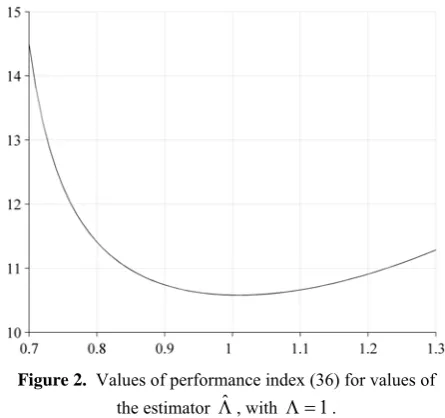
for a particular Λˆ , are shown in Figure 2. One can see that the resulting graph can be described with great precision by a quadratic function with different coeffi-cients for positive and negative errors, which in fact proves that over- and underestimation of the parameter Λ have other results on the performance index value.
Figure 2. Values of performance index (36) for values of
the estimator Λˆ , with Λ =1.
To use an analogous methodology to that of the linear case considered in the previous section, the loss function is assumed in quadratic and asymmetrical form defined as
2 2
ˆ ˆ
( ) for 0
ˆ ( , )
ˆ ˆ
( ) for 0
a x x x x l x x
b x x x x
⎧ − − ≤
= ⎨
− − ≥
⎩ , (38)
while the coefficients a and b are positive and not necessarily equal to each other. Thus, the Bayes loss function (2) is given by the formula
ˆ
2 2
ˆ
ˆ ˆ ˆ
( ) ( ) ( ) d ( ) ( ) d
x B
x
l x a x x f x x b x x f x x ∞
−∞
=
∫
− +∫
− . (39)One can show that the function lB attains its minimum at the value xˆ being a solution of the equation
ˆ
ˆ ˆ
( ) ( ) ( ) d ( ) ( ) d 0
x
a b x x f x x a x x f x x ∞
−∞ −∞
−
∫
− −∫
− = . (40)This solution exists and is unique. As in the linear case, dividing the above equation by b, note that it is necessary to identify only the ratio of the parameters a and b.
( ) d
xK x x ∞
−∞
< ∞
∫
(41)be given. Besides the functions Ui introduced in Sec-tion 3.1, let for any fixed i=1, 2, ... , m the functions
:R R
i
V → be defined as
1
( ) d
x
i i
y x V x yK y
h−∞ h
−
⎛ ⎞
= ⎜ ⎟
⎝ ⎠
∫
. (42)The kernel K should be chosen so the function
:R R
J → such that J x( )=
∫
−∞x y K y( ) dy be expres-sed by a convenient analytical formula.If an expected value is estimated by the arith-metical mean value of a sample, then criterion (40) can be described equivalently as
1
ˆ ˆ ˆ ˆ
[( )( ( ) ( )) ] 0
m
i i i
i
a b xU x V x ax axm =
− − + − =
∑
. (43)If the left-hand side of the above formula is denoted by L x( )ˆ , then – using the equality V xi′( )ˆ =xU xˆ i′( )ˆ directly resulting from dependencies (21) and (42) – one can express the value of its derivative as
1
ˆ ˆ
( ) m [( ) i( )]
i
L x a b U x am =
′ =
∑
− − . (44)In this situation, the solution of criterion (40) can be calculated numerically on the basis of Newton’s algo-rithm (24)-(25).
In the quadratic case also Cauchy kernel (27) is proposed; then formula (28) remains true and addi-tionally for the general form of the kernel estimator (14):
2
2
1 1
( ) arctg
π 2 π 1 (45) π 1 i i i i i i i i i i i x x
x x hs
V x x
hs x x
hs hs x x hs ⎛ ⎞ − ⎜ ⎟ ⎜ ⎛ − ⎞ ⎟ ⎜ ⎟ = ⎜ ⎟+ + ⎡ ⎤ ⎜ ⎝ ⎠ ⎛ − ⎞ ⎟ ⎢ + ⎥ ⎜ ⎜ ⎟ ⎟ ⎜ ⎢⎣ ⎝ ⎠ ⎥⎦ ⎟ ⎝ ⎠ − ⎡ ⎛ − ⎞ ⎤ ⎢ + ⎜ ⎟ ⎥ ⎢ ⎝ ⎠ ⎥ ⎣ ⎦ .
Also dependencies (29)-(35) remain unchanged. Primary investigations concerning the quadratic case, including also the multidimensional, were pub-lished in the article [14].
3.3. Higher Degree Polynomial Case
In this section, detailed investigations presented earlier will be supplemented with the polynomial case, that is where the loss function is an asymmetrical mo-nomial of the order k≥2 and is therefore given by the following formula:
⎪⎩ ⎪ ⎨ ⎧ ≥ − − ≤ − − − = 0 ˆ for ) ˆ ( 0 ˆ for ) ˆ ( ) 1 ( ) , ˆ ( x x x x b x x x x a x x
l k kk , (46)
while the coefficients a and b are positive, and may differ. Criterion for the optimal estimator ˆx is given here in the form
1
ˆ ˆ
1
ˆ
( 1) ( ) ( ) d
ˆ
( ) ( ) d 0
k k
x x
k
ak x x f x x
bk x x f x x
∞ − − −∞ − − + − =
∫
∫
. (47)
The solution of the above equation exists and is unique. When the statistical kernel estimators are used with respect to the density f , it is possible again to create an efficient numerical algorithm enabling equa-tion (47) to be solved. Let the kernel K be continuous, of positive values and fulfilling the following condi-tion:
1 ( ) d
k
x K x x
∞ − −∞
< ∞
∫
. (48)For clarity of presentation, the case k=3 is pre-sented below. Thus, equation (47) takes on the equiva-lent form
ˆ ˆ ˆ
2 2
2 2
ˆ ˆ
( ) ( ) d 2 ( ) d ( ) d
ˆ 2ˆ ( ) d ( ) d 0
x x x
a b x f x x x x f x x x f x x
a x x x f x x x f x x
−∞ −∞ −∞ ∞ ∞ −∞ −∞ ⎛ ⎞ + ⎜ − + ⎟ ⎝ ⎠ ⎛ ⎞ − ⎜ − + ⎟= ⎝ ⎠
∫
∫
∫
∫
∫
. (49)
Now, with any fixed i=1, 2, … , m, let the functions Ui and Vi defined by dependencies (21) and (42) be given, and furthermore Wi:R→R be introduced as
2
1
( ) d
x
i i
y x
W x y K y
h−∞ h
−
⎛ ⎞
= ⎜ ⎟
⎝ ⎠
∫
. (50)Making use of the above notations, condition (49) can be expressed in the following form
(
2)
1
2
( ) ( ) 2 ( ) ( ) 2
lim ( ) 0
m
i i i i
i
i x
a b x U x xV x W x ax x
W x amx = →∞ ⎡ + − + + ⎣ ⎤ − ⎦− =
∑
. (51)
If the left-hand side of the above formula is denoted as ( )
L x , then – also taking into account the equalities
( ) ( )
i i
V x′ =xU x′ and W xi′( )=xV xi′( ) resulting from dependencies (21), (42) and (50) – the derivative of the function L is
(
)
1
( ) 2( ) ( ) ( ) 2
2
m
i i i
i
L x a b xU x V x ax
amx =
′ = ⎡⎣ + − + ⎤⎦
−
∑
. (52)while the functions L and L′ are given by formulas (51)-(52).
The Cauchy kernel (27) must by modified here to the form
2 3
8 1
( )
3π(1 )
K x
x
=
+ . (53)
An increase of the power in the denominator has been implied with the necessity of ensuring the fulfillment of condition (48). Here for the general form of the kernel estimator (14):
3
2 2
2 2
5 ( )
π 1 3π 1
1arctg 1
π 2 i i i i i i i i i i i
x x x x
hs hs
U x
x x x x
hs hs x x hs ⎛ − ⎞ − ⎜ ⎟ ⎝ ⎠ = + ⎛ ⎛ − ⎞ ⎞ ⎛ ⎛ − ⎞ ⎞ ⎜ +⎜ ⎟ ⎟ ⎜ +⎜ ⎟ ⎟ ⎜ ⎝ ⎠ ⎟ ⎜ ⎝ ⎠ ⎟ ⎝ ⎠ ⎝ ⎠ ⎛ − ⎞ + ⎜ ⎟+ ⎝ ⎠ (54) 2 2 2 ( ) 3π 1 i i i i hs V x x x hs = − ⎡ ⎛ − ⎞ ⎤ ⎢ + ⎜ ⎟ ⎥ ⎢ ⎝ ⎠ ⎥ ⎣ ⎦ 3 2 2 2 2 5
π 1 3π 1
1 1 arctg π 2 i i i i i i i i i i i
x x x x
hs hs
x
x x x x
hs hs x x hs ⎛ ⎛ − ⎞ ⎜ − ⎜ ⎟ ⎜ ⎝ ⎠ ⎜ + + ⎜ ⎡ ⎛ − ⎞ ⎤ ⎡ ⎛ − ⎞ ⎤ ⎜ ⎢ +⎜ ⎟ ⎥ ⎢ +⎜ ⎟ ⎥ ⎜ ⎢⎣ ⎝ ⎠ ⎥⎦ ⎢⎣ ⎝ ⎠ ⎥⎦ ⎝ ⎞ ⎛ − ⎞ + ⎜ ⎟+ ⎟⎟ ⎝ ⎠ ⎠ (55) 2 2 4 ( )
3π 1
i i i i i hs x W x x x hs = − ⎡ ⎛ − ⎞ ⎤ ⎢ + ⎜ ⎟ ⎥ ⎢ ⎝ ⎠ ⎥ ⎣ ⎦ 3 2 2 2 2 2 5
π 1 3π 1
1 1 arctg π 2 i i i i i i i i i i i
x x x x
hs hs
x
x x x x
hs hs x x hs ⎛ ⎛ − ⎞ ⎜ − ⎜ ⎟ ⎜ ⎝ ⎠ ⎜ + + ⎜ ⎡ ⎛ − ⎞ ⎤ ⎡ ⎛ − ⎞ ⎤ ⎜ ⎢ +⎜ ⎟ ⎥ ⎢ +⎜ ⎟ ⎥ ⎜ ⎢⎣ ⎝ ⎠ ⎥⎦ ⎢⎣ ⎝ ⎠ ⎥⎦ ⎝ ⎞ ⎛ − ⎞ + ⎜ ⎟+ ⎟⎟ ⎝ ⎠ ⎠ (56) 3 2 2 2 2 2 2
3π 1 3π 1
1 arctg 1
3π 6
i i i i i i i i i i i
x x x x
hs hs
h s
x x x x
hs hs x x hs ⎛ ⎛ − ⎞ ⎜ − ⎜ ⎟ ⎜ ⎝ ⎠ ⎜ + − ⎜ ⎡ ⎛ ⎞ ⎤ ⎡ ⎛ ⎞ ⎤ − − ⎜ ⎢ +⎜ ⎟ ⎥ ⎢ +⎜ ⎟ ⎥ ⎜ ⎢ ⎝ ⎠ ⎥ ⎢ ⎝ ⎠ ⎥ ⎣ ⎦ ⎣ ⎦ ⎝ ⎞ ⎛ − ⎞ + ⎜ ⎟+ ⎟⎟ ⎝ ⎠ ⎠ .
The constants used within the plug-in method are: 1
( ) 3
P K = (57)
7 ( )
4π
R K = ; (58)
dependencies (31)-(35) remain unchanged.
The above investigations can be similarly trans-posed to a higher order of asymmetrical polynomial loss function (1), although on account of their extreme nature, they seem to be useful mainly for atypical ap-plicational tasks.
4. Numerical Simulations Results
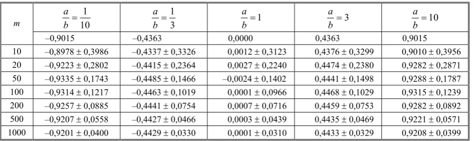
The correctness of the algorithm designed here has been checked in detail using a numerical simulation. The results are shown below for five values of the ratio a b=1 10, 1 3, 1, 3, 10. Investigations were carried out for m = 10, 20, 50, 100, 200, 500, 1000. In every case 1000 samples were obtained, and the tables below display mean and standard deviation values of results calculated on the basis of these samples, de-scribed using the standard notation „mean value ± standard deviation”.
First, it was assumed that the uncertainty of the es-timated parameter has standard normal distribution:
) 1 , 0 (
N ; (59)
in the hereafter-used natural notation N(μ,σ) denotes normal distribution with the expected value μ∈R and the standard deviation σ>0. The above classical example of distribution (59) is taken at the beginning only for its simplicity and ease of interpretation – in such a simple case use of the complex nonparametric estimation method is in practice redundant.
In Tables 1 and 2 results are compared for twinned quadratic and cubic cases, respectively. The theoretical value of the estimator is shown here below the values of the ratio a b.
considered distribution (59) these values are opposite with respect to those obtained for a b=1 3). When
10
a b= this effect is again intensified – the values of
the investigated estimator are 0,901 and 0,716, re-spectively.
Table 1. Results for distribution (59) for the quadratic case (k = 2)
10 1
=
b a
3 1
=
b a
1
=
b a
3
=
b a
0 1
=
b a
m
–0,9015 –0,4363 0,0000 0,4363 0,9015 10 –0,8978 ± 0,3986 –0,4337 ± 0,3326 0,0012 ± 0,3123 0,4376 ± 0,3299 0,9010 ± 0,3956 20 –0,9223 ± 0,2802 –0,4415 ± 0,2364 0,0027 ± 0,2240 0,4474 ± 0,2380 0,9282 ± 0,2871 50 –0,9335 ± 0,1743 –0,4485 ± 0,1466 –0,0024 ± 0,1402 0,4441 ± 0,1498 0,9288 ± 0,1787 100 –0,9314 ± 0,1217 –0,4463 ± 0,1019 0,0001 ± 0,0966 0,4468 ± 0,1029 0,9315 ± 0,1239 200 –0,9257 ± 0,0885 –0,4441 ± 0,0754 0,0007 ± 0,0716 0,4459 ± 0,0753 0,9282 ± 0,0892 500 –0,9207 ± 0,0558 –0,4427 ± 0,0466 0,0003 ± 0,0439 0,4435 ± 0,0469 0,9221 ± 0,0571 1000 –0,9201 ± 0,0400 –0,4429 ± 0,0330 0,0001 ± 0,0310 0,4433 ± 0,0329 0,9208 ± 0,0399
Table 2. Results for distribution (59) for the cubic case (k = 3)
10 1
=
b a
3 1
=
b a
1
=
b a
3
=
b a
0 1
=
b a
m
–0,7158 –0,3436 0,0000 0,3436 0,7158 10 –0,6812 ± 0,3926 –0,3293 ± 0,3485 0,0012 ± 0,3340 0,3310 ± 0,3469 0,6802 ± 0,3893 20 –0,7267 ± 0,2882 –0,3473 ± 0,2528 0,0029 ± 0,2434 0,3526 ± 0,2562 0,7305 ± 0,2949 50 –0,7550 ± 0,1860 –0,3614 ± 0,1591 –0,0023 ± 0,1517 0,3566 ± 0,1591 0,7495 ± 0,1846 100 –0,7609 ± 0,1303 –0,3623 ± 0,1093 –0,0004 ± 0,1034 0,3612 ± 0,1093 0,7587 ± 0,1302 200 –0,7574 ± 0,0944 –0,3597 ± 0,0801 0,0013 ± 0,0764 0,3623 ± 0,0808 0,7601 ± 0,0964 500 –0,7540 ± 0,0596 –0,3584 ± 0,0499 0,0010 ± 0,0476 0,3604 ± 0,0510 0,7567 ± 0,0623 1000 –0,7543 ± 0,0443 –0,3588 ± 0,0365 0,0004 ± 0,0344 0,3597 ± 0,0365 0,7554 ± 0,0442
Comparing further results for the quadratic and cubic cases one can note that in the former the values of the estimator are closer to zero. This effect is in-tuitively justified, as for large arguments, the values of the cubic function are greater than the quadratic, and consequently, the tendency to eliminate extreme re-sults appears. It is also worth noticing that estimator values in the linear case for a b=1 10, 1/3, 1, 3, 10 equal –1,335, –0,675, 0, 0,675, 1,335, respectively, which is additionally confirmed in the above inter-pretation.
Similar conclusions can be drawn for the next dis-tribution under research:
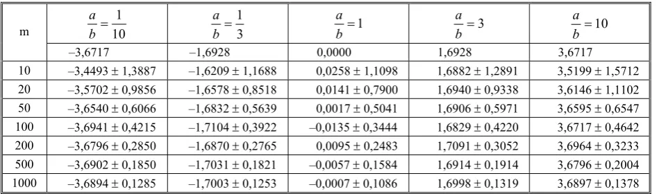
0,25 ( 5, 2) 0,5 (0, 1) 0,25 (5, 2)N − + N + N . (60) The obtained results are shown in Table 3. This distri-bution is trimodal. Its expectation value equals 0, and the standard deviation is 15 3,9≅ , so almost four times greater than that for distribution (59). On con-sideration of this fact one can infer that the results are comparative to those previously obtained for distribu-tion (59), presented in Table 1. It should be concluded that the accuracy of estimation does not generally de-pend on the number of the modal values of the inves-tigated distribution. Despite a significant change in the type of distribution examined, the procedure for
calcu-lating the estimator did not change in any way. This is due to the application of the nonparametric statistical kernel estimators methodology, the use of which is in practice independent of the distribution under research. In every case represented by specific columns in Tables 1-3, together with the increase in the random sample size m, the average error of the estimation and its standard deviation decrease to zero. From an appli-cational point of view these are fundamental pro-perties required of estimators used in practice. Above all this trait means that, as the size of samples in-creases, the obtained estimator values tend to the theo-retical, while their “dispersion” decreases. This allows any assumed precision to be acquired, albeit after en-suring the proper sample size. This in practice implies a necessity to reach a compromise between these two quantities. A satisfactory degree of precision was ob-tained when the size of the sample was between 10 and 200, i.e. for m∈[10, 200]; in particular, the large values became necessary when the difference between parameters a and b increased.
Table 3. Results for distribution (60) for the quadratic case (k = 2)
10 1
=
b a
3 1
=
b a
1
=
b a
3
=
b a
0 1
=
b a
m
–3,6717 –1,6928 0,0000 1,6928 3,6717 10 –3,4493 ± 1,3887 –1,6209 ± 1,1688 0,0258 ± 1,1098 1,6882 ± 1,2891 3,5199 ± 1,5712 20 –3,5702 ± 0,9856 –1,6578 ± 0,8518 0,0141 ± 0,7900 1,6940 ± 0,9338 3,6146 ± 1,1102 50 –3,6540 ± 0,6066 –1,6832 ± 0,5639 0,0017 ± 0,5041 1,6906 ± 0,5971 3,6595 ± 0,6547 100 –3,6941 ± 0,4215 –1,7104 ± 0,3922 –0,0135 ± 0,3444 1,6829 ± 0,4220 3,6717 ± 0,4642 200 –3,6796 ± 0,2850 –1,6870 ± 0,2765 0,0095 ± 0,2483 1,7091 ± 0,3052 3,6964 ± 0,3233 500 –3,6902 ± 0,1850 –1,7031 ± 0,1821 –0,0057 ± 0,1584 1,6914 ± 0,1914 3,6796 ± 0,2004 1000 –3,6894 ± 0,1285 –1,7003 ± 0,1253 –0,0007 ± 0,1086 1,6998 ± 0,1319 3,6897 ± 0,1378
In the case of the time-optimal control problem considered in Section 3.1, approximating the loss function from Figure 1 by an asymmetrical linear function with a b=15 5, , the feedback controller based on the procedure proposed here had a signifi-cant – even to about 40% – advantage over the classi-cal controller based on the value of the mean.
For the optimal control task with the quadratic per-formance index from Section 3.2, the loss function shown in Figure 2 was assumed in the asymmetrical quadratic form with a b=5 2, . For those realizations for which the system seemed to be stable, the cont-roller based on the procedure proposed here also had a significant – even to about 50% – advantage with re-spect to the one using the mean value. Moreover, there was a greater distance from the instability area. In the case of the feedback controller obtained with the estimator worked out here, the system became unstable for the value of the object parameter Λ ≅1,7, although in the case of the system designed using the mean value, this had already happened for Λ ≅1,5.
5. Conclusions
This article has presented the method of estimating the values of model parameters, dedicated to those cases where the dependence of losses implied by esti-mation error can be approximated by asymmetrical and polynomial function. Asymmetry here represents the different influences of under- and overestimation of the parameter’s estimator on the value of these losses, whereas the degree of the polynomial signifies how acceptable large errors are. The method worked out here is universal in character and can be applied in many areas of science and practice, also outside engi-neering.
To find the distribution of the uncertainty measure of an estimated parameter, statistical kernel estimators were used, which made the investigated procedure independent of distribution type. The solution was based on the Bayes decision rule, which allows a minimum – generally understood – average losses value to be obtained. As a result the complete algo-rithm was worked out, enabling the value of the
esti-mator to be calculated on the basis of the measure-ments of the examined quantity, and the definition of degree – often natural in practical applications – of the polynomial and the ratio of the values of a losses func-tion’s coefficients. The herein-presented procedure is complete, and its practical implementation requires neither detailed knowledge of the theoretical aspects nor laborious research.
Although the uncertainty of the examined parame-ter was considered in the most common probabilistic approach, the worked out method can also be used for other types of uncertainty, for example that based on fuzzy logic [7]. In this case one is able to calculate the value of the optimal defuzzyficator or the preference function [5] – the procedure proposed here allows the Bayes preference function for fuzzy numbers to be obtained.
The propriety of the presented algorithms has been verified numerically. Thus, depending on the relation between the coefficients of the loss function, the esti-mator’s value properly changed to one of smaller losses, while the size of this change was defined by the polynomial degree. As the random sample size increased, the average error of the estimation and its standard deviation tended to zero.
One may construe that the benefits arising from application of the method proposed in this paper are greater the more complex the control system is, and over- and under-estimation of model’s parameters have a more differing influence on performance index, i.e. when asymmetry of the loss function is more distinct.
References
[1] M. Athans, P.L. Falb. Optimal Control.
McGraw-Hill, New York, 1966.
[2] J.O. Berger. Statistical Decision Theory.
Springer-Verlag, New York, 1980.
[3] A. van den Bos. Parameter Estimation for Scientists
and Engineers. Wiley, Hoboken, 2007.
[4] J. Caldwell, Y.M. Ram. Mathematical Modelling.
Concepts and Case Studies, Springer, Berlin, 1999.
[5] J. Fodor, M. Roubens. Fuzzy Preference Modelling
[6] D. Kincaid, W. Cheney. Numerical Analysis. Brooks/ Cole, Pacific Grove, 2002.
[7] J. Kacprzyk. Multistage Fuzzy Control: A
Model-Based Approach to Control and Decision-Making. Wiley, Chichester, 1997.
[8] P. Kulczycki. Estymatory jadrowe w analizie
syste-mowej. WNT, Warsaw, 2005.
[9] P. Kulczycki. An Algorithm for Bayes Parameter
Identification. Journal of Dynamic Systems, Measure-ment, and Control, Vol. 123, 2001, 611-614.
[10] P. Kulczycki. Estymatory jadrowe w zagadnieniach
badan systemowych. P. Kulczycki, O. Hryniewicz, J. Kacprzyk (eds.), Techniki informacyjne w badaniach systemowych, WNT, Warsaw, 2007, 79-105.
[11] P. Kulczycki. Kernel Estimators in Industrial
Applica-tions. B. Prasad (ed.), Soft Computing Applications in Industry, Springer-Verlag, Berlin, 2008, 69-91.
[12] P. Kulczycki. Applicational Possibilities of
Nonpara-metric Estimation of Distribution Density for Control Engineering. Bulletin of the Polish Academy of Sci-ences, Technical SciSci-ences, Vol. 56, 2008, 347-359.
[13] P. Kulczycki, M. Charytanowicz. Asymmetrical
Conditional Bayes Parameter Identification for Cont-rol Engineering. Cybernetics and Systems, Vol. 39, 2008, 229-243.
[14] P. Kulczycki, A. Mazgaj. An algorithm for Bayes
parameter identification with quadratic asymmetrical loss function. Control and Cybernetics, Vol. 34, 2005, 1127-1148.
[15] P. Kulczycki, A. Mazgaj. Bayes Parameter
Identifi-cation with Polynomial Asymmetrical Loss Function. Proceedings of the 17th World Congress IFAC, Seoul, 6-11 July 2008, 12395-12400, CD: 12395.
[16] P. Kulczycki, R. Wisniewski. Fuzzy Controller for a
System with Uncertain Load. Fuzzy Sets and Systems, Vol. 131, 2002, 185-195.
[17] L. Ljung. System Identification: Theory for the User.
Prentice Hall, Englewood Cliffs, 1998.
[18] F. Morrison. The Art of Modeling Dynamic Systems.
Multiscience Press, New York, 1991.
[19] H.E. Nusse, J.A. Yorke. Dynamics: Numerical
Ex-plorations. Springer-Verlag, New York, 1997.
[20] B.W. Silverman. Density Estimation for Statistics and
Data Analysis. Chapman and Hall, New York, 1986.
[21] T.S. Soderstrom, P. Stoica. System Identification.
Prentice Hall, Englewood Cliffs, 1994.
[22] M.P. Wand, M.C. Jones. Kernel Smoothing.
Chap-man and Hall, London, 1995.