Deep Augmentation in Convolutional Neural Network

DEEP AUGMENTATION IN

CONVOLUTIONAL NEURAL NETWORKS

By

ASIM NEUPANE

Bachelor of Engineering in Computer Engineering Tribhuvan University

Kathmandu,Nepal 2013

Submitted to the Faculty of the Graduate College of Oklahoma State University

in partial fulfillment of the requirements for

the Degree of MASTER OF SCIENCE

DEEP AUGMENTATION IN

CONVOLUTIONAL NEURAL NETWORKS

Thesis Approved:

Dr. Christopher John Crick Thesis Advisor Dr. Nophill Park

Name: Asim Neupane Date of Degree: May 2018

Title of Study: Deep Augmentation in Convolutional Neural Networks Major Field: Computer Science

Abstract: Deep Convolutional Neural Networks (ConvNets) have been tremendously successful in the field of computer vision, particularly in image classification and object recognition tasks. A huge amount of training data, computing power and training time are needed to train such networks. Data augmentation is a technique commonly used to help address the data scarcity problem. Although augmentation helps with the problem of training data scarcity to some extent, huge amounts of computing power and training time are still needed. In this work, we propose a novel approach of training deep ConvNets, which reduces the need for huge computing power and training time. In our approach, we move data augmentation deep in the network and perform augmentation of high-level features rather than raw input data. Our experiment shows that performing augmentation in feature space reduces the training time and even the computing power. Moreover, we can break down our model into two parts (pre-argumentation and post-augmentation) and train one part at a time. This allows us to train a bigger model in a system than it could normally handle.

TABLE OF CONTENTS Chapter Page 1 Introduction 1 1.1 Proposed Approach . . . 2 1.2 Outline of Thesis . . . 3 2 Literature Review 4 3 Technical Approach & Architecture 9 3.1 Overview of General ConvNet Archtitecure . . . 9

3.2 Problems in General ConvNet Architecture . . . 10

3.3 Proposed Architecture . . . 10 4 Experiments 14 4.1 Datasets . . . 14 4.2 ConvNet Models . . . 15 4.2.1 MNIST Model . . . 15 4.2.2 CIFAR10 Model . . . 17 4.3 Hyper-Parameters . . . 17 4.3.1 Padding . . . 17 4.3.2 Activation . . . 18 4.3.3 Pooling . . . 18 4.3.4 Kernel . . . 19 4.3.5 Optimizer . . . 19 4.3.6 Initialization . . . 20 4.4 Data Augmentation . . . 21

5 Simulation and Results 22

6 Discussion 27

LIST OF TABLES

Table Page

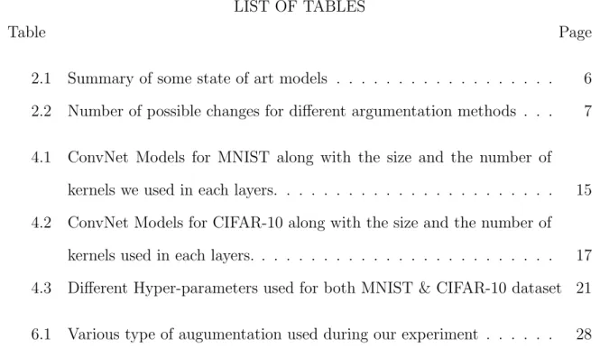
2.1 Summary of some state of art models . . . 6 2.2 Number of possible changes for different argumentation methods . . . 7 4.1 ConvNet Models for MNIST along with the size and the number of

kernels we used in each layers. . . 15 4.2 ConvNet Models for CIFAR-10 along with the size and the number of

kernels used in each layers. . . 17 4.3 Different Hyper-parameters used for both MNIST & CIFAR-10 dataset 21 6.1 Various type of augumentation used during our experiment . . . 28

LIST OF FIGURES

Figure Page

2.1 Revolution of Depth [He et al. ILSVRC 2015 presentation] . . . 5

3.1 Architecture of AlexNet . . . 10

3.2 Architecture of Proposed Method . . . 11

3.3 Proposed Architecture . . . 11

3.4 Detail Architecture of Proposed Method . . . 12

3.5 Detail of Proposed Method . . . 13

3.6 Some example representations of data deep in the network . . . 13

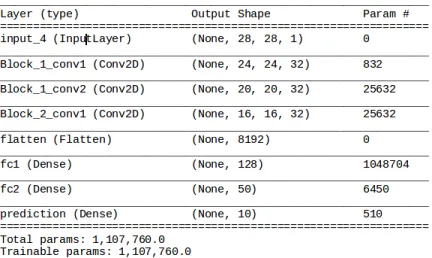
4.1 Summary of MNIST model A showing how the shape of input varies as the image goes deep into the network, and the number of parameters learned in each layer. . . 15

4.2 Summary of MNIST model B showing how the shape of input varies as the image goes deep into the network, and the number of parameters learned in each layer . . . 16

4.3 Summary of MNIST model C showing how the shape of input varies as the image goes deep into the network, and the number of parameters learned in each layer. . . 16

4.4 Summary of CIFAR10 model A showing how the shape of input varies as the image goes deep into the network and the number of parameters learned in each layer. . . 18

4.5 Summary of CIFAR10 model B showing how the shape of input varies as the image goes deep into the network & number of parameters learned in each layer. . . 19 4.6 Summary of CIFAR10 Model C showing how the shape of input varies

as the image goes deep into the network and the number of parameters learned in each layer. . . 20 5.1 Graph showing the training accuracy and training time of different

MNIST baseline models . . . 23 5.2 Graph showing the training accuracy and training time of different

CIFAR-10 baseline models . . . 24 5.3 Graph showing the variation in training accuracy and training time

when performing data augmentation in different blocks deep in the network for MNIST model A . . . 24 5.4 Graph showing the variation in training accuracy and training time

when performing data augmentation in different blocks deep in the network for MNIST model B. . . 25 5.5 Graph showing the variation in training accuracy and training time

when performing data augmentation in different blocks deep in the network for MNIST model C. . . 25 5.6 Graph showing the variation in training accuracy and training time

when performing data augmentation in different blocks deep in the network for CIFAR-10 model A. . . 25 5.7 Graph showing the variation in training accuracy and training time

when performing data augmentation in different blocks deep in the network for CIFAR-10 model B. . . 26

5.8 Graph showing the variation in training accuracy and training time when performing data augmentation in different blocks deep in the network for CIFAR-10 model C. . . 26 6.1 Graph showing the variation in test accuracy of MNIST models when

performing data augmentation in different blocks deep in the network. 27 6.2 Graph showing variation in test accuracy of CIFAR-10 models when

CHAPTER 1

Introduction

Artificial Intelligence (AI), in recent years, has brought lots of interest in research community again. Apart from research community, even tech companies are showing interest in this field. Companies ranging from tech giants like Google, Facebook, Microsoft, etc. to small start-up companies are using artificial intelligence in their work and even investing a huge amount of funds in this area.

Several factors are responsible for this renewed interest in the field of AI: (i) the increase in computing capability available in powerful Graphical Processing Units (GPU) (1), which made the training of large models practical. (ii) Availability of large training datasets (18)(27)(24). (iii) Tweaking of previous concepts and methods such as activation functions (9)(15)(7), optimization functions like stochastic gradient descent with momentum (20) and RMSProp (22).

Along with the recent rise of AI, Convolutional Neural Network (ConvNets) mod-els (13) have extended the state of art. Particularly in the area of image classification and recognition (8)(23)(21)(19)(11) they have outperformed all other previous mod-els.

Efficiently training ConvNets is a complex task. Practitioners face many chal-lenges such as fixing hyper-parameters including the number of layers, the size of filters, stride size, etc. Apart from these challenges, one basic challenge in training these deep ConvNets is the amount of training data they require. ConvNets require a huge amount of data to generalize. It is similar to the phrase the more you see the more you know. To address this challenge, the most commonly used method is Data

Augmentation that is, to perform some kind of transformation on the input images and feed it to the network to increase the data. Data Augmentation is widely used by the research community (11). It has helped a lot to train deep ConvNets with compar-atively little available input data. Although the use of Data Augmentation expands the training examples, it poses a greater challenge in terms of computational power as well as training time. We think this method can be improved to get better training time with fewer learn-able parameters and enable the training of larger ConvNets than the training system would normally able to handle using current methods.

In this work, we develop an efficient method for training ConvNets. Our emphasis is on minimizing the training time and minimizing the learnable parameters.

1.1 Proposed Approach

In the general current approach for training deep a ConvNet, data augmentation is performed in the actual images. Therefore, data augmentation is done before the input is fed to the ConvNet input layer.

In the proposed method, we first feed the input to the network and get a higher order representation of the image. Then we perform the augmentation of that high-level representation of the image before training the rest of the network with the augmented data.

One of the challenges in the proposed method is finding the appropriate layer for performing the augmentation. We are addressing this challenge by training the net-works on different type of datasets, visualizing their output layers, and performing the augmentation of them. Then we generalize the method for finding the appro-priate layer based on our simulation result. Another challenge in this approach is: determining what type of data-augmentation scheme best suits for performing aug-mentscheme.ation of feature space? For this, we applied various type of commonly used augmentation scheme and found a set of most effective augmentation

1.2 Outline of Thesis

The structure of this thesis is as follows: chapter 2 provides a literature review of ConvNets, data augmentation, and different methods used to speed up the ConvNet training process. chapter 3 presents our technical approach and discuss the proposed method to speed up training of ConvNets.Chapter 4 deals with the experiment we performed. In chapter 5, we present our result. Finally, in chapter 6 we discuss our experiment and obtained results and in chapter 7, we draw our conclusions.

CHAPTER 2

Literature Review

A Convolutional Neural Network (ConvNet) (14) is an artificial neural network that uses convolutional operations in at least one layer of the network. ConvNets models are a stack of convolutional, activation and pooling layers with fully connected linear classifier layers at the end of the network for classification. ConvNet have attracted much attention over the last few years due to their capability of inducing rich fea-tures. Particularly, when ConvNets are trained on large scale data these networks have shown great efficiency and have advanced the state of art on traditional vision problems such as classification, object recognition (11) (19)(21) and object detection (5)(17).

The graph in figure 2.1 shows the top five classification methods on the ImageNet dataset by different models submitted to the ILSVRC (ImageNet Large Scale Visual Recognition Challenge) image classification and object detection challenge at large scale. The graph in figure 2.1 clearly shows that at the current state of the art deeper models show better performance.

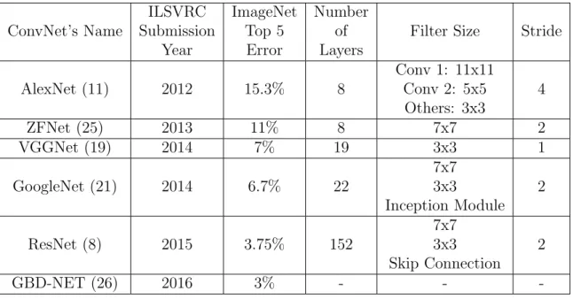
Table 2.1 shows that the along with increasing the depth, increasing the width of the network helps to obtain the better results (21)(8). Moreover, it also shows the trend of decreasing filter size and stride.

Increasing the depth of a network is a promising way to enhance the performance of ConvNets but on the downside, this leads to growth in the number of parameters and model complexity. In this work, we propose a better method for training ConvNets, which reduces the number of learnable parameters and decreases the training time.

Figure 2.1: Revolution of Depth [He et al. ILSVRC 2015 presentation]

Deeper ConvNets are often prone to overfitting. Data Augmentation is one of the most used methods to overcome this problem. It enforces robustness of a learning system to variations in the input. It has played an active role in achieving state-of-art results on many vision tasks. The practice of fine-tuning existing pre-trained Con-vNets is also a commonly used method when only a little training data are available. However, it fails in few-shot and one shot learning scenarios (20). In these scenarios, very few data are available perhaps only one example per class. Thus, fine-tuning millions of parameters of the pre-trained model is not possible. Moreover, to use the pre-trained model, we have to find a model that has been trained on data similar to our problem domain, which may not be available. Hence, the only reliable way of solving the problem of limited data is to augment the data available.

AlexNet (11) the winner of ILSVRC 2012, used two types of data augmentation. The first form of augmentation used image translations and horizontal reflections, which helped them to increase their training set data by the factor of 2048. The second form of augmentation they used was Principal Component Analysis (PCA). Krizhevsky et al. claim that this scheme reduces the top-1 error rate by over 1%.

ConvNet’s Name ILSVRC Submission Year ImageNet Top 5 Error Number of Layers

Filter Size Stride

AlexNet (11) 2012 15.3% 8 Conv 1: 11x11 Conv 2: 5x5 Others: 3x3 4 ZFNet (25) 2013 11% 8 7x7 2 VGGNet (19) 2014 7% 19 3x3 1 GoogleNet (21) 2014 6.7% 22 7x7 3x3 Inception Module 2 ResNet (8) 2015 3.75% 152 7x7 3x3 Skip Connection 2 GBD-NET (26) 2016 3% - -

-Table 2.1: Summary of some state of art models

Andrew G. Howard in his work on improving deep ConvNets for image classifica-tion, (10) proposed two additional transformations that extend translation invariance and color invariance. As the first method, he proposed a smart way of cropping the training data. Particularly, he first scaled the smallest side to some fixed size (in his case he scaled to 256), which gave him 256xN or Nx256 sized image. Then, he used fixed crop size (224x224 in his case). This gave him a large number of additional training examples and helped the network to learn more extensive translation invari-ance. As a second method, he used random manipulation of contrast, brightness, and color and claimed that this helps to generate examples that cover a span of image variations, which will help neural network to learn invariance to changes in these properties.

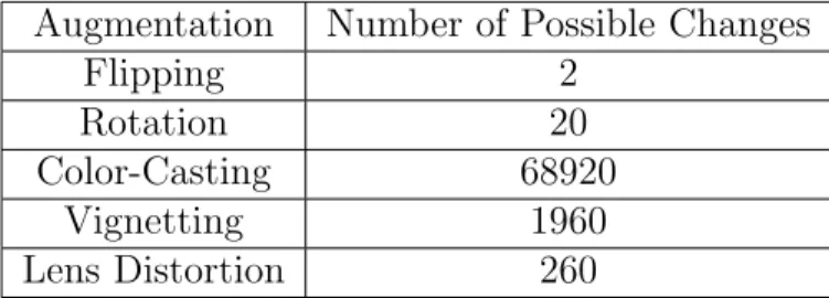
Baidu researchers, Ren et al. worked on scaling up image recognition. They (23) used Vignetting (making the periphery of an image darker compared to the center part of the image) and lens distortion (deviation from rectilinear projection caused by lenses), in addition to augmentation scheme in AlexNet and in work of Andrew

G. Howard. The table 2.2 shows the number of changes for different augmentation methods.

Augmentation Number of Possible Changes

Flipping 2

Rotation 20

Color-Casting 68920

Vignetting 1960

Lens Distortion 260

Table 2.2: Number of possible changes for different argumentation methods

All the works described above proposed some clever way for augmenting the data but they do not deal with finding the appropriate layer and performing the augmen-tation task on it. In this work, we estimate the best place for performing the data augmentation and perform the augmentation in that layer of the network rather than performing the augmentation before feeding to the network.

In recent years, some work has been done that closely aligns with our work. These methods focus on improving the performance of neural networks by improving the efficiency of data augmentation.

The work of Mattis et al. (16) claims that not all form of transformations are equally informative. Their work proposed an algorithm, Image Transformation Pur-suit (ITP) that automatically selects a compact set of transformations.

In 2016, Alhussein et al. (4) proposed automatic and adaptive algorithms for choosing the transformation of the samples used in data augmentation. Particularly, in this work, they presented a novel Data Augmentation approach where small trans-formations are sought to maximize the classifiers loss.

Mandar et al. (3) proposed attribute-guided augmentation (AGA) that learns a mapping, which allows synthesizing data such that an attribute of the synthesized sample is at the desired strength. Here, first, they train an R-CNN (Region-based Convolutional Network) detector to identify objects in 2D images and then train the network regressors which gives 3D attribute (depth and pose information) of a de-tected object.

In 2017 Terrance et. al. (2) used an LSTM-based (Long Short Term Memory) (a kind of recurrent network that can long-term dependencies) and sequence auto-encoder in order to learn feature space from the available training data then performed argumentation on them by adding random noise. In this work, we are taking advan-tage of the hierarchical feature learning property of ConvNet to obtain features which are simple and easier to train as compared to an LSTM based auto-encoder. More-over, we also find the appropriate layer for data augmentation.

While the previous works are mostly focused on the choice of data augmentation strategy, our work is different in that we move the data augmentation layer deep in the network and perform only the required calculation. Moreover, our approach can take advantage of the various choice of data augmentation strategy discussed earlier.

CHAPTER 3

Technical Approach & Architecture

In this chapter, we first revisit the basic form of a modern Convolutional Neural Network (ConvNet) architecture that is widely used in practice. Then we introduce the proposed architecture and finally, compare the two architectures.

3.1 Overview of General ConvNet Archtitecure

ConvNets are neural networks with some convolution operation. A convolution op-eration is defined as:

s(t) = (x∗w)(t) (3.1)

Where, x is a input

w is a kernel function

t is a particular instant of time

In our experiment, the input is a multidimensional array so we need to have a multi-dimensional kernel. Therefore, Equation 3.1 becomes:

s(i, j) = (I∗K)(i, j) =X m X n I(m, n)K(i−m, j−n) (3.2) Where, I is a multidimensional input

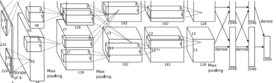
Figure 3.1: Architecture of AlexNet

The ConvNet architecture consist of multiple stacks of layers having convolution operations as stated in Equation 3.2, activation layers which adds non-linearity to the output and pooling layers which output the summary statistics of nearby activations and helps to make representation invariant to small change in input. Generally at the end of this stack we have a fully connected linear classifier.

Figure 3.1 shows the architecture of (11) (winner of ImageNet challenge 2012). In the architecture shown in figure 3.1, we can see that input is taken, then the entire network is trained on that input, and this process is continued for each input we have in our dataset. This process is also known as total learning.

3.2 Problems in General ConvNet Architecture

In our general approach, we train the entire network at once with each image in our dataset; we end up learning lots of parameters which leads to long training times, which is the bottleneck for modern ConvNet. There is need of huge amounts of memory to store all the parameters. Moreover, the use at data augmentation to increase the training data increases the need for computational power and memory.

3.3 Proposed Architecture

In order to mitigate the concerns discussed in section 3.2, we propose the new training methodology.

training data we have. This is also true even for the entire set of augmented data samples generated. In the proposed method, we move the augmentation layer deep in the network and perform only the required computation.

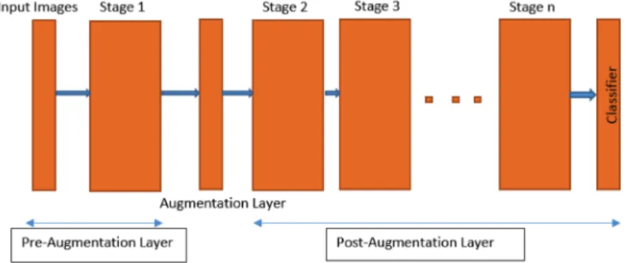
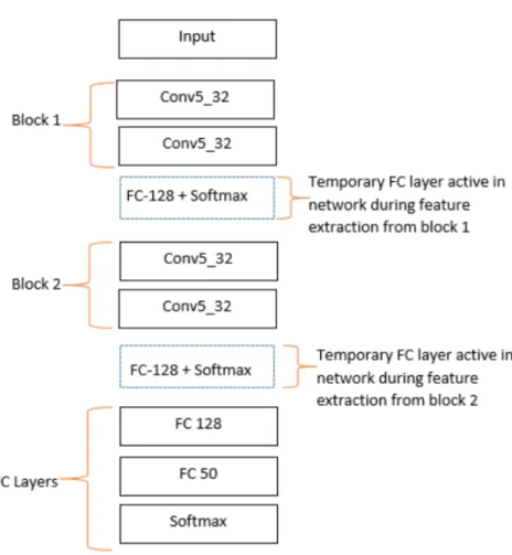
First, we group the convolutional, activation and pooling layer as one block and then move the data augmentation layer to each block in turn to find the most ap-propriate layer for data augmentation. The figure 3.2 shows the basic architecture of the proposed method, with the augmentation layer placed after the first stage of the network.

Figure 3.2: Architecture of Proposed Method

Then we move the augmentation deeper in the network one-step at a time to find the most appropriate stage for placing the augmentation layer. During the training, we back propagate only until the stage after augmentation and train only the part of the network after augmentation layer. This is shown in figure 3.3 & 3.4.

Figure 3.3: Proposed Architecture

Moreover, during training we break our models into two parts (pre-argumentation & post-augmentation) and train one part at a time. We train the pre-augmentation

Figure 3.4: Detail Architecture of Proposed Method

part first. To train just the pre-augmentation part, we added a temporary fully connected layer and extracted feature space data from a layer before a fully con-nected layer then we perform the augmentation on these features and train the post-augmentation part. This enable us to train a bigger network than a system would normally be able to handle.

Before training the pre-argumentation part to extract features, we first group the data based on their class and pass the data to the network on the basis of class ( i.e all the data of particular class were trained once then we moved to next class); this helped us to get labels of data even in the feature space. Then, we shuffled the feature space data and performed augmentation on them and trained the post-augmentation part of the network.

Figure 3.5 shows detailed information of our implementation for MNIST Model C. We followed same approach for training all our models shown in table 4.1 & table 4.2. Figure 3.6 shows examples of how the data looks like deep in the network.

Figure 3.5: Detail of Proposed Method

CHAPTER 4

Experiments

We divided our experiment into two phases.

First, we find an appropriate layer for data augmentation. For this, we train the ConvNet with different datasets by placing the augmentation layer in different layers and record the accuracy, training time and numbers of parameters for each run. Finally, we compare the accuracy, training time and numbers of parameters learned for each movement of the augmentation layer and generalize the best layer for performing the augmentation.

Secondly, we place the augmentation layer in the position obtained from the first phase of our experiment and compare the accuracy, training time and number of parameters learned for three approaches: fixed size ConvNet model with no augmen-tation, with augmentation before feeding to the network, and ConvNet with aug-mentation deep in the network for each of the training methods described in section 3.

4.1 Datasets

We used following datasets for our experiments:

• MNIST is a dataset of handwritten digits. Images of this dataset are 28x28 greyscale image. This dataset has 60, 0000 training examples and a test set of 10,000 examples.

Figure 4.1: Summary of MNIST model A showing how the shape of input varies as the image goes deep into the network, and the number of parameters learned in each layer.

6000 images per class. It has a training set of 50,000 images and a test set of 10,000 images.

4.2 ConvNet Models

For our experiments, we have used the models:

4.2.1 MNIST Model

Since, MNIST consist of grayscale images, we will be using the models shown in Table 4.1. Figure 4.1, 4.2 & 4.3 shows the summary of baseline model for model A, B & C respectively. A B C Conv5-32 Conv5-32 Conv5-32 Conv5-32 Conv5-32 Conv5-32 Conv5-32 Conv5-32 Conv5-32 FC 128 —— FC 50 —— Softmax

Table 4.1: ConvNet Models for MNIST along with the size and the number of kernels we used in each layers.

Figure 4.2: Summary of MNIST model B showing how the shape of input varies as the image goes deep into the network, and the number of parameters learned in each layer

Figure 4.3: Summary of MNIST model C showing how the shape of input varies as the image goes deep into the network, and the number of parameters learned in each layer.

4.2.2 CIFAR10 Model

Since, CIFAR10 consist of colored images, we will be using the models shown in Table 4.2. Figure 4.4, 4.5 and 4.6 show the summary of baseline models for model A, B and C respectively. A B C Conv5-64 Conv5-64 Conv5-128 MaxPool(2,2) (Stride of 2) Conv5-64 Conv5-128 MaxPool(2,2) (Stride of 2) Conv3-128 MaxPool(2,2) (Stride of 2) Conv3-128 Conv3-128 MaxPool(2,2) (Stride of 2) Conv3-128 Conv3-128 MaxPool(2,2) (Stride of 2) Conv3-256 Conv3-256 Conv3-256 MaxPool(2,2) (Stride of 2) Conv3-256 Conv3-256 Conv3-256 MaxPool(2,2) (Stride of 2) Conv3-512 MaxPool(2,2) (Stride of 2) Conv3-512 Conv3-512 MaxPool(2,2) (Stride of 2) Conv3-512 Conv3-512 Conv3-512 MaxPool(2,2) (Stride of 2) FC 512 —— FC 128 —— Softmax

Table 4.2: ConvNet Models for CIFAR-10 along with the size and the number of kernels used in each layers.

4.3 Hyper-Parameters

4.3.1 Padding

After the convolution operation, the size of representation shrinks so we need to pad the inputs to train the deeper ConvNet. During our experiment, we used no padding for MNIST dataset but for CIFAR-10, we used zero padding in order to maintain the size of the image in high dimension, as our CIFAR-10 models are deeper as compared to MNIST models because after each convolution operation spatial size decreases.

Figure 4.4: Summary of CIFAR10 model A showing how the shape of input varies as the image goes deep into the network and the number of parameters learned in each layer.

For zero-padding we added zeros around the border of the image. We added this in such a way that the convolution operation does not decrease the size of the image. For no-padding mode we did not use any padding so the size of image decreased after each convolution operation.

4.3.2 Activation

We used Rectifier Linear Units (ReLu) as our activation function which thresholds outputs to 0. ReLu computes the function:

f(x) =max(0, x) (4.1)

4.3.3 Pooling

Pooling layers reduce the spatial size of the representation. They reduce the amount of parameters and computation in the network and also summarize the response over

Figure 4.5: Summary of CIFAR10 model B showing how the shape of input varies as the image goes deep into the network & number of parameters learned in each layer. the whole neighborhood. In this experiment, we applied max-pooling with filter size 2x2 with a stride of 1.

4.3.4 Kernel

In this experiment during convolution operation, we used a kernel size of 5x5 in the initial layers and kernel size of 3x3 in later layers.

4.3.5 Optimizer

The goal of optimization is to find the set of weights that minimizes the loss function. We used Adam (19) as the optimizer in this experiment.

Figure 4.6: Summary of CIFAR10 Model C showing how the shape of input varies as the image goes deep into the network and the number of parameters learned in each layer.

4.3.6 Initialization

In this experiment we initialized all the kernel using He uniform initialization (10). This is a uniform variance initializer that draws samples from a uniform distribution within [-limit to limit] where limit is:

limit =sqrt(6/f an in) (4.2)

Where, fan in is the number of input units in the weight tensor.

samples from a uniform distribution within [-lim to lim].

lim=sqrt(6/(f an in+f an out) (4.3)

Where, fan in is units in the weight tensor fan out is output units in the weight tensor

Table 4.3 presents the summary of hyper-parameters we used during the experi-ment.

Augmentation Scheme Rescaling & Horizontal Flip Initialization Glorot & He Form

Activation ReLu

Learning Rate 0.001

Optimizer adam

Table 4.3: Different Hyper-parameters used for both MNIST & CIFAR-10 dataset

4.4 Data Augmentation

Finding the data augmentation scheme for feature space data was one of our chal-lenges. During our experiment, we visualized the output of each layer, while visual-izing we found that to some depth features resembles more like the actual image (as shown in figure 3.6). So for our experiment, we decided to try out with some of the commonly used data augmentation schemes for augmenting images. Table 6.1 shows the list of data augmentation we tried. From this list, we were interested in finding the best set of augmentations that can be applied to the different feature levels.

CHAPTER 5

Simulation and Results

In the first phase of our experiment, we were interested in finding the best layer for the data augmentation. For this, we placed our argumentation layer after each block and recorded the model performance.

In the experiment, we first trained our baseline models for both MNIST and CIFAR-10. For the baseline model, we used data-augmentation before feeding data into the network.

Table 4.1 shows the basic architecture of our MNIST models and figure 5.3, 5.4 and 5.5 show more detail about of each of our MNIST models. Particularly, figure 5.3, 5.4 and 5.5 show the types and number of layers in our model, the number of parameters learned at each layer and also shows how our input size changes in each layer. The graph in figure 5.1 shows the training time and accuracy of our MNIST baseline models.

Table 4.2 shows the basic architecture of our CIFAR-10 models and figure 5.6 , 5.7 and 5.8 show more detail summary. The graph in figure 5.2 show the training time and accuracy of our CIFAR-10 baseline models. Particularly, figure 5.6 , 5.7 and 5.8 show types and number of layers in our model, the number of parameters learned at each layer and how our input size changes in each layer.

After training the baseline model, we moved the data augmentation layer one block deeper into the network and trained the network again.

The graphs in figure 5.3, 5.4 & 5.5 show the training time and accuracy of our MNIST Models when we placed augumentation deep in the network.

Figure 5.1: Graph showing the training accuracy and training time of different MNIST baseline models

The graphs in figure 5.6, 5.7 & 5.8 show the training time and accuracy of our CIFAR-10 Models when we placed argumentation deep into the network.

In second phase of our experiment, we were interested in finding most efficient set of data augmentation scheme for augmenting the feature space data. There are number of ways to argument a data. In this work we tested with most commonly used argumentation schemes that are frequently used for images. Table 6.1 shows the list of argumentation schemes we used during our experiment. Since we were looking for the set of augmentation schemes that can be applied to the different levels of feature space data, we applied a different combination of augmentation scheme shown in the table 6.1 to a different level of features and trained the network. Our experiment showed that scaling and horizontal flip produced better data because models trained with these data gave a better prediction. So, we concluded that for image datasets like MNIST and CIFAR-10, scaling and horizontal flipping produced better synthetic data and used these two augmentation scheme for our experiment.

Figure 5.2: Graph showing the training accuracy and training time of different CIFAR-10 baseline models

Figure 5.3: Graph showing the variation in training accuracy and training time when performing data augmentation in different blocks deep in the network for MNIST model A

Figure 5.4: Graph showing the variation in training accuracy and training time when performing data augmentation in different blocks deep in the network for MNIST model B.

Figure 5.5: Graph showing the variation in training accuracy and training time when performing data augmentation in different blocks deep in the network for MNIST model C.

Figure 5.6: Graph showing the variation in training accuracy and training time when performing data augmentation in different blocks deep in the network for CIFAR-10 model A.

Figure 5.7: Graph showing the variation in training accuracy and training time when performing data augmentation in different blocks deep in the network for CIFAR-10 model B.

Figure 5.8: Graph showing the variation in training accuracy and training time when performing data augmentation in different blocks deep in the network for CIFAR-10 model C.

CHAPTER 6

Discussion

Similar to the mammalian visual cortex, ConvNets learn features in the form of a hierarchy. Therefore, ConvNets learn general features in the initial layers and gradually learn more specific features towards the final layers (12). Keeping this in mind at the initial phase we thought the model would achieve best results by performing augmentation towards the end of the network. During the first phase of our experiment, we found that augmentation performed before fully connected layers will comparable training accuracy but the testing error decreases as compared to augmentation on other blocks. The graphs in Figure 5.3 to 5.8 show the variation in training accuracy (includes the pre-augmentation and post augmentation training time) as we move data augmentation deeper into the network.

The graphs in Figure 6.1 to 6.2 show the variation in test accuracy as we move data augmentation deeper into the network for our MNIST and CIFAR-10 models. From our experiment, we found that it is more efficient to perform augmentation towards the middle of the network rather than at the beginning of network. But during our

Figure 6.1: Graph showing the variation in test accuracy of MNIST models when performing data augmentation in different blocks deep in the network.

Figure 6.2: Graph showing variation in test accuracy of CIFAR-10 models when performing data augmentation in different blocks deep in the Network.

experiment we discovered, if we moved argumentation too deep in the network then test accuracy decreases. This decrease in accuracy might be the augumentation of over zoomed image by convolution operation which failed to produce the meaningful data.

For the second phase of our experiment, we placed the augmentation layer towards the middle of the network and performed different sets of augumentation. Here, we were more concerned about using few numbers of augumentation schemes and still be-ing able to train our model properly and achieve better accuracy. Table 6.1 shows the list of argumentation schemes we tried during our experiment. Among these schemes, we found rescaling and horizontal flipping are the best choices for augmenting both MNIST and CIFAR-10 dataset we used in our experiment.

Augmentation Scheme Explanation

Feature-wise standard normalization Divided input data by standard deviation of dataset Sample-wise standard normalization Divided each input by its standard deviation

ZCA whitening applied zca whitening

Horizontal flip randomly flipping image horizontally Vertical flip randomly flipping image vertically

Rotation Randomly rotated image in the range of 0 to 180 Rescale Rescaled image by the factor of 1/255 Table 6.1: Various type of augumentation used during our experiment

CHAPTER 7

Conclusion

In this work, we seek to optimize the commonly used training process of ConvNets. We proposed a new approach for training deep ConvNets. Particularly, in our method move the augmentation layer deep in the network by finding the appropriate layer for performing data augmentation.

We analyzed the effect of moving data augmentation deep in the network. We demon-strate our the technique on two commonly used datasets (MNIST and CIFAR-10).We achieved near state of the art results for both the dataset, using the simple models shown in table 4.1 and 4.2.

The most important elements of our study are: First, our experiment showed data augmentation deep on the network is more fruitful than performing it in the beginning of the network. Second, we investigated and presented the most appropriate layer for performing augmentation of feature space data. Finally, we found best set of data augmentation schemes from a list commonly used data augmentation schemes. The proposed method helps to train ConvNets in less time and with fewer parame-ters as compared to the general approach. Moreover, the method helps to train larger ConvNets than the training system would normally able to handle.

In the future, we hope to implement our approach on a much more challenging dataset. We hope to perform augmentation on features with very little or almost no domain specific knowledge and train ConvNets faster with comparatively little computing power.

BIBLIOGRAPHY

[1] Dan C Cire¸san, Ueli Meier, Jonathan Masci, Luca M Gambardella, and J¨urgen Schmidhuber. High-performance neural networks for visual object classification.

arXiv preprint arXiv:1102.0183, 2011.

[2] Terrance DeVries and Graham W Taylor. Dataset augmentation in feature space.

arXiv preprint arXiv:1702.05538, 2017.

[3] Mandar Dixit, Roland Kwitt, Marc Niethammer, and Nuno Vasconcelos. Aga: Attribute guided augmentation. arXiv preprint arXiv:1612.02559, 2016.

[4] Alhussein Fawzi, Horst Samulowitz, Deepak Turaga, and Pascal Frossard. Adap-tive data augmentation for image classification. InImage Processing (ICIP), 2016 IEEE International Conference on, pages 3688–3692. IEEE, 2016.

[5] Ross Girshick. Fast r-cnn. InProceedings of the IEEE International Conference on Computer Vision, pages 1440–1448, 2015.

[6] Xavier Glorot and Yoshua Bengio. Understanding the difficulty of training deep feedforward neural networks. InProceedings of the Thirteenth International Con-ference on Artificial Intelligence and Statistics, pages 249–256, 2010.

[7] Ian J Goodfellow, David Warde-Farley, Mehdi Mirza, Aaron C Courville, and Yoshua Bengio. Maxout networks. ICML (3), 28:1319–1327, 2013.

[8] Kaiming He, Xiangyu Zhang, Shaoqing Ren, and Jian Sun. Deep residual learn-ing for image recognition. arXiv preprint arXiv:1512.03385, 2015.

[9] Kaiming He, Xiangyu Zhang, Shaoqing Ren, and Jian Sun. Delving deep into rectifiers: Surpassing human-level performance on imagenet classification. In

Proceedings of the IEEE International Conference on Computer Vision, pages 1026–1034, 2015.

[10] Andrew G Howard. Some improvements on deep convolutional neural network based image classification. arXiv preprint arXiv:1312.5402, 2013.

[11] Alex Krizhevsky, Ilya Sutskever, and Geoffrey E Hinton. Imagenet classification with deep convolutional neural networks. In Advances in neural information processing systems, pages 1097–1105, 2012.

[12] Yann LeCun. Learning invariant feature hierarchies. InComputer vision–ECCV 2012. Workshops and demonstrations, pages 496–505. Springer, 2012.

[13] Yann LeCun, L´eon Bottou, Yoshua Bengio, and Patrick Haffner. Gradient-based learning applied to document recognition. Proceedings of the IEEE, 86(11):2278– 2324, 1998.

[14] Yann LeCun, Koray Kavukcuoglu, Cl´ement Farabet, et al. Convolutional net-works and applications in vision. In ISCAS, pages 253–256, 2010.

[15] Vinod Nair and Geoffrey E Hinton. Rectified linear units improve restricted boltzmann machines. In Proceedings of the 27th International Conference on Machine Learning (ICML-10), pages 807–814, 2010.

[16] Mattis Paulin, J´erˆome Revaud, Zaid Harchaoui, Florent Perronnin, and Cordelia Schmid. Transformation pursuit for image classification. In Proceedings of the IEEE Conference on Computer Vision and Pattern Recognition, pages 3646– 3653, 2014.

[17] Shaoqing Ren, Kaiming He, Ross Girshick, and Jian Sun. Faster r-cnn: Towards real-time object detection with region proposal networks. In Advances in neural information processing systems, pages 91–99, 2015.

[18] Olga Russakovsky, Jia Deng, Hao Su, Jonathan Krause, Sanjeev Satheesh, Sean Ma, Zhiheng Huang, Andrej Karpathy, Aditya Khosla, Michael Bernstein, et al. Imagenet large scale visual recognition challenge. International Journal of Com-puter Vision, 115(3):211–252, 2015.

[19] Karen Simonyan and Andrew Zisserman. Very deep convolutional networks for large-scale image recognition. arXiv preprint arXiv:1409.1556, 2014.

[20] Ilya Sutskever, James Martens, George E Dahl, and Geoffrey E Hinton. On the importance of initialization and momentum in deep learning. ICML (3), 28:1139–1147, 2013.

[21] Christian Szegedy, Wei Liu, Yangqing Jia, Pierre Sermanet, Scott Reed, Dragomir Anguelov, Dumitru Erhan, Vincent Vanhoucke, and Andrew Rabi-novich. Going deeper with convolutions. In Proceedings of the IEEE Conference on Computer Vision and Pattern Recognition, pages 1–9, 2015.

[22] Tijmen Tieleman and Geoffrey Hinton. Lecture 6.5-rmsprop: Divide the gradient by a running average of its recent magnitude. COURSERA: Neural Networks for Machine Learning, 4(2), 2012.

[23] Ren Wu, Shengen Yan, Yi Shan, Qingqing Dang, and Gang Sun. Deep image: Scaling up image recognition. arXiv preprint arXiv:1501.02876, 7(8), 2015. [24] Jianxiong Xiao, Krista A Ehinger, James Hays, Antonio Torralba, and Aude

Oliva. Sun database: Exploring a large collection of scene categories. Interna-tional Journal of Computer Vision, pages 1–20, 2014.

[25] Matthew D Zeiler and Rob Fergus. Visualizing and understanding convolutional networks. InEuropean conference on computer vision, pages 818–833. Springer, 2014.

[26] Xingyu Zeng, Wanli Ouyang, Junjie Yan, Hongsheng Li, Tong Xiao, Kun Wang, Yu Liu, Yucong Zhou, Bin Yang, Zhe Wang, et al. Crafting gbd-net for object detection. arXiv preprint arXiv:1610.02579, 2016.

[27] Bolei Zhou, Agata Lapedriza, Jianxiong Xiao, Antonio Torralba, and Aude Oliva. Learning deep features for scene recognition using places database. InAdvances in neural information processing systems, pages 487–495, 2014.

VITA ASIM NEUPANE Candidate for the Degree of

Master of Science

Thesis: Deep Augmentation in Convolutional Neural Networks Major Field: Computer Science

Biographical:

Personal Data: Born in Ilam, Nepal in March 1992. Education:

Received a Bachelors of Engineering in Computer Engineering at Tribhuvan University in December 2013.

Completed the requirements for the degree of Master of Science with a major in Computer Science at Oklahoma State University in May 2018.