econstor
www.econstor.eu
Der Open-Access-Publikationsserver der ZBW – Leibniz-Informationszentrum Wirtschaft
The Open Access Publication Server of the ZBW – Leibniz Information Centre for Economics
Nutzungsbedingungen:
Die ZBW räumt Ihnen als Nutzerin/Nutzer das unentgeltliche, räumlich unbeschränkte und zeitlich auf die Dauer des Schutzrechts beschränkte einfache Recht ein, das ausgewählte Werk im Rahmen der unter
→ http://www.econstor.eu/dspace/Nutzungsbedingungen nachzulesenden vollständigen Nutzungsbedingungen zu vervielfältigen, mit denen die Nutzerin/der Nutzer sich durch die erste Nutzung einverstanden erklärt.
Terms of use:
The ZBW grants you, the user, the non-exclusive right to use the selected work free of charge, territorially unrestricted and within the time limit of the term of the property rights according to the terms specified at
→ http://www.econstor.eu/dspace/Nutzungsbedingungen By the first use of the selected work the user agrees and declares to comply with these terms of use.
zbw
Leibniz-Informationszentrum WirtschaftWohltmann, Hans-Werner; Winkler, Roland C.
Working Paper
On the Non-Optimality of Information: An Analysis of
the Welfare Effects of Anticipated Shocks in the New
Keynesian Model
Economics working paper / Christian-Albrechts-Universität Kiel, Department of Economics, No. 2008,21
Provided in cooperation with:
Christian-Albrechts-Universität Kiel (CAU)
Suggested citation: Wohltmann, Hans-Werner; Winkler, Roland C. (2008) : On the Non-Optimality of Information: An Analysis of the Welfare Effects of Anticipated Shocks in the New Keynesian Model, Economics working paper / Christian-Albrechts-Universität Kiel, Department of Economics, No. 2008,21, http://hdl.handle.net/10419/27676
On the Non-Optimality of Information:
An Analysis of the Welfare Effects of
Anticipated Shocks in the
New Keynesian Model
by Hans-Werner Wohltmann and Roland Winkler
No 2008-21
Economics Working Paper
On the Non-Optimality of Information:
An Analysis of the Welfare Effects of Anticipated Shocks in
the New Keynesian Model
Hans-Werner Wohltmann‡and Roland Winkler§
Department of Economics, Christian-Albrechts-University of Kiel, Olshausenstr. 40, D-24098 Kiel, Germany
December 29, 2008
Abstract
This paper compares the welfare effects of anticipated and unanticipated cost-push shocks in the canonical New Keynesian model with optimal mon-etary policy. We find that, for empirically plausible degrees of nominal rigidity, the anticipation of a future cost-push shock leads to a higher wel-fare loss than an unanticipated shock. A welwel-fare gain from the anticipation of a future cost shock may only occur if prices are sufficiently flexible. We analytically show that this surprising result holds although unanticipated shocks lead to higher negative impact effects on welfare than anticipated shocks.
JEL classification: E31, E32, E52
Keywords: Anticipated Shocks, Optimal Monetary Policy, Sticky Prices, Welfare Analysis
‡Corresponding author: Phone: ++49-431-880-1449, Fax: ++49-431-880-2228, E-mail: [email protected]
1
Introduction
Does theanticipation of future shocks has a stabilizing effect on the economy and thus reduces the welfare loss compared to unanticipated shocks? In this paper, we seek to answer this question by comparing the welfare effects of unanticipated and anticipated cost-push shocks in the canonical New Keynesian model with a monetary authority which minimizes a standard loss function that weights the volatility of inflation and the output gap. In particular, we analytically solve for dynamics and welfare in case of optimal monetary policy under timeless perspective commitment and discretion. We distinguish the usual case of unanticipated cost-push shocks and the case of future cost-push shocks that are known in advance.
Since the real business cycle revolution of Kydland and Prescott (1982) and his successors, unanticipated random disturbances are considered as the main driving force in explaining business cycles. New Keynesians add nominal rigidities to the real business cycle framework to study the role of monetary policy in aggregate fluctuations but maintain the assumption of unpredictable random shocks (see, e.g., the textbooks of Walsh (2003), Woodford (2003), or Gal´ı (2008)). An exception is the stream of literature that analyzes anticipated disinflations going back to Ball (1994) who shows that a simple variant of the New Keynesian model predicts a boom in response to an anticipated disinfla-tion. However, the literature on the optimal design of monetary policy usually considers unanticipated shocks (see, e.g. Clarida, Gal´ı, and Gertler (1999), Svensson (1999), King, Khan, and Wolman (2000), or Woodford (2003)).
Recently, a number of macroeconometric studies emphasize the role of antic-ipated shocks as sources of macroeconomic fluctuations. Beaudry and Portier (2006) find that more than half of business cycle fluctuations are caused by news about future technological opportunities. Davis (2007) and Fujiwara, Hi-rose, and Shintani (2008) analyze the importance of anticipated shocks in large scale DSGE models closely related to the model of Christiano, Eichenbaum, and Evans (2005) and report that these disturbances are important components of aggregate fluctuations. Schmitt-Groh´e and Uribe (2008) conduct a Bayesian es-timation of a real-business cycle model and find that anticipated shocks are the most important source of aggregate fluctuations. In particular, they report that anticipated shocks explain two thirds of the volatility in consumption, output, investment, and employment.
Theoretical studies on the role of anticipations for business cycle fluctuations include Beaudry and Portier (2004, 2007), Beaudry, Collard, and Portier (2006), Jaimovich and Rebelo (2006, 2008), Den Haan and Kaltenbrunner (2007), or Christiano, Ilut, Motto, and Rostagno (2008).
However, none of these studies considers the welfare effects of the antic-ipation of future shocks. In this study, we derive a solution of welfare as a function of the time span between the anticipation and the realization of the shock which enables us to discover the dependency of welfare on the length of the anticipation period. Furthermore, we contribute to the literature by sys-tematically investigating the role of nominal rigidities for the welfare impacts of anticipations.
To the best of our knowledge, Wohltmann and Winkler (2008) and Winkler (2008) are the only studies that compare the welfare effects of anticipated and unanticipated shocks. They both analyze energy price shocks under different monetary policy regimes including optimal monetary policy. However, these studies rely on numerical simulations and do not, as we do, investigate the role of nominal rigidities.
The main results of this paper are the following. For empirically plausible degrees of nominal rigidity, the anticipation of a future cost-push shock leads to a higher welfare loss than an analogous unanticipated shock. A welfare gain from the anticipation of a future cost shock may only occur if prices are suffi-ciently flexible. This result is consistent with the findings of Schmitt-Groh´e and Uribe (2008) who show that the anticipation of future shocks has a stabilizing effect on an economy without nominal rigidities. We point out that precisely the degree of nominal rigidity play an important role for the evaluation of the welfare effects of anticipations.
Our results are driven by two opposing effects. On the one hand, we obtain the well-known result that the anticipation of a future shock dampens its im-pact effect. On the other hand, we show that anticipation of future cost-push shocks enhances the persistence of output and inflation and thus enhances the welfare loss. This persistence effect, in turn, is amplified by the degree of price stickiness.
Nevertheless, at a first glance, our findings seem to be puzzling since it suggests that the information about the occurrence of future shocks is in general welfare-reducing. But then the question arises, why rational agents do not ignore the knowledge about future disturbances. In the remainder of this paper, we will seek to shed more light on this question.
Our paper is organized as follows. Section 2 presents the canonical New Keynesian model and its solution under the policy regimes timeless perspective commitment and discretion. In section 3, we report and discuss our main find-ings. Furthermore, we provide analytical proofs and, for the sake of illustration, numerical simulations. Section 4 concludes. The paper includes an extensive mathematical appendix.
2
The Framework
The canonical New Keynesian model serves as analytical framework. It consists of an optimizing IS-type relationship of the form
xt=Etxt+1−
1
σ(it−Etπt+1) (σ≥1) (1)
and a price adjustment equation of Calvo-Rotemberg type, often referred to as New Keynesian Phillips Curve (NKPC)
πt=βEtπt+1+κxt+kt (0< β <1, κ >0) (2)
xtdenotes the output gap,πtis inflation, anditis the nominal interest rate. Et
discount factor and 1/σ denotes the intertemporal elasticity of substitution. It is well-known that under the assumptions of Calvo (1983) price setting, a constant returns to scale production function with labor as single input, and perfect labor markets, the slope parameterκis given byκ= (η+σ)(1−ω)(1ω−βω), whereη is the inverse of the labor supply elasticity.1 Obviously,κ is negatively correlated with the degree of price rigidity ω. According to the Calvo price adjustment mechanism, a fraction 1−ωof firms can adjust their price in period
t. Simultaneously,ω is the probability that a single price which is reoptimized in period t, also holds in the next period t+ 1. The Calvo parameter ω is therefore a measure of the degree of price rigidity on the goods markets.
In the NKPC, kt represents a temporary cost-push shock that is assumed
to be autoregressive of order one with AR parameterϕ∈[0,1) and a one-unit cost shockεt
kt=ϕkt−1+εt (t≥T >0) (3)
Since we consider anticipated cost-push shocks, the one-unit cost shockεtis not
white noise, but known to the public before the shock actually occurs.2 Assume
that at time t = 0 the public anticipates the cost-push shock to take place at some future timeT >0. Then,
εt=
(
1 fort=T >0
0 fort6=T (4)
The adjustment dynamics induced by anticipated shocks involve two phases, the time span between the anticipation and the realization of the shock (0≤ t < T) and the time span after the implementation of the shock (T ≤t≤ ∞). The lead timeT up to the realization of the shock is equal to the length of the anticipation phase 0≤ t < T. An implication of our definition of anticipated shocks is that rational expectations are equivalent to perfect foresight so that we can omit the expectations operator.
The policy maker’s objective at the time of anticipationt= 0 is to minimize the intertemporal loss function
V =E0
∞
X
t=0
βt(α1πt2+α2x2t) (α1> α2 >0, 0< β≤1) (5)
which reflects the objective of flexible inflation targeting (see, e.g., Svensson (1999)). Rotemberg and Woodford (1999) and Woodord (2003) show that, under certain conditions, a quadratic loss function in inflation and the output gap is the correct approximation to the representative agent’s utility function. The first-order conditions of the policy problem under timeless perspective precommitment monetary policy as well as under discretion are well known and
1
See, e.g., Walsh (2003) for a derivation of the NKPC under Calvo pricing.
2
Schmitt-Groh´e and Uribe (2007) study the impacts of anticipated cost shocks on the pass-through to prices.
need not to be derived here (see, for example, Walsh (2003)). Under the optimal timeless perspective precommitment policy, inflation satisfies the targeting rule
πt=−
α2
α1κ
(xt−xt−1) (6)
while the output gap is described by the second-order difference equation
1 +β+ α1κ 2 α2 xt−xt−1−βEtxt+1 =− α1κ α2 kt (7)
where the expectational operator can be omitted in case of anticipated shocks. To solve the difference equation forxt, write equation (7) as
xt+1 wt+1 =C xt wt + α1κ α2β 0 kt (8) wherewt=xt−1 and C= 1 β 1 +β+α1κ2 α2 −β1 1 0 ! (9)
The auxiliary variable wt is backward-looking (with the initial value w0 = 0,
while the output gapxt is forward-looking. The system matrixC has two real
eigenvalues r1 and r2 with r1 > 1 > r2 > 0 so that the Blanchard and Kahn
(1980) saddlepath stability condition is satisfied. A detailed derivation of our results is provided in the mathematical appendix.
The solution for the output gap over the anticipation phase is given by
xt=− 1 r1−ϕ 1 r1−r2 α1κ α2β r1−T(r1t+1−rt2+1) for t < T (10) with the initial values
x0 =− 1 r1−ϕ α1κ α2β r−T 1 , x−1 = 0 (11)
while the solution fort≥T is defined by
xt= α1κ α2β 1 (r1−ϕ)(r2−ϕ) · (12) · " ϕt+1−T −(r1−ϕ)r −T 2 −(r2−ϕ)r1−T r1−r2 rt2+1 # fort≥T
In the limiting case of unanticipated shocks (T = 0), the term in brackets in equation (12) simplifies toϕt+1−rt+1
2 . Note that the solution formula (10) also
holds in the shock periodt=T.
Using (6), the solution time path of the inflation rate follows
πt= 1 β 1 r1−ϕ 1 r1−r2 r1−T (r1−1)rt1−(r2−1)rt2 fort≤T (13)
with the initial value π0 = 1 β 1 r1−ϕ r1−T (14) and πt= 1 β 1 r1−ϕ 1 r2−ϕ · (15) · " (1−ϕ)ϕt−T −(r1−ϕ)r −T 2 −(r2−ϕ)r−1T r1−r2 (1−r2)r2t # fort≥T
In the limiting caseT = 0, the term in brackets simplifies to (1−ϕ)ϕt−(1−r 2)r2t.
To determine the welfare loss under the optimal precommitment policy, write the loss functionV as V1+V2, where
V1 =E0 T−1 X t=0 βt α1πt2+α2x2t (16)
is the loss in the anticipation period and
V2=E0 ∞ X t=T βt α1πt2+α2x2t (17)
is the loss caused by the realization of the shock.
By inserting the solution forxtand πt, the lossV1 can be rewritten as
V1 =α1λ2r1−2T r1T −rT2 r1−1 rT 2 + 1−r2 rT 1 (18) where λ= 1 β 1 r1−ϕ 1 r1−r2 (19) Accordingly, the lossV2 can be rewritten as
V2 = α1βT β2(r 1−ϕ)2 ( rT 2 −r1T 2 (1−r2) (r1−r2)2r12T + r1 r1r2−ϕ2 ) (20)
The total lossV is then simply given by V =V1+V2.
Under the policy regime discretion (D), the central bank is unable to make a commitment to future policies. Now private expectations are given for the central bank and the reduced form of the first-order conditions reads as
πt=− α2 α1κ xt (21) Etxt+1= 1 β 1 +α1κ 2 α2 xt+ α1κ α2β kt (22)
withEtxt+1=xt+1 in case of anticipated shocks. The difference equation inxt
has the unstable eigenvalue
rD = 1 β 1 +α1κ 2 α2 = 1 α2β α2+α1κ2 >1 (23)
and the forward solution
xt=− ∞ X s=0 rD−s 1 rD α1κ α2β kt+s (24) Since kt+s= ( ϕt+s−T fort+s≥T 0 fort+s < T (25) we obtain fort≥T xt=− α1κ α2+α1κ2−α2βϕ ϕt−T (26) and fort < T xt=− α1κ α2+α1κ2−α2βϕ rDt−T (27)
Due to rDt−T = 1 for t = T, the solution formula (27) also holds in the shock periodt=T. Fort= 0 we obtain
x0=−
α1κ
α2+α1κ2−α2βϕ
rD−T (28)
so that the the size of the initial jump ofxt decreases with increasing T.
For the inflation rate πt we obtain the solution time path
πt= α2 α2+α1κ2−α2βϕ rtD−T if 0≤t≤T α2 α2+α1κ2−α2βϕ ϕt−T if t≥T (29)
Note that the limiting caseϕ= 0 impliesπt=xt= 0 for t > T.
It is well-known that the loss under discretion (VD) is greater than the total
loss under the optimal precommitment policy. By inserting the solution time paths forπtand xtin the loss function, we obtain
VD =V1D+V2D (30) = T−1 X t=0 βt α22 α1κ2 +α2 x2t + ∞ X t=T βt α22 α1κ2 +α2 x2t = α1α2[α2+α1κ 2] [α2(1−βϕ) +α1κ2]2 r−D2T −βT 1−βr2 D + β T 1−βϕ2 ! = α1α2[α2+α1κ 2] [α2(1−βϕ) +α1κ2]2 1 1−βr2 D rD−2T −β(r 2 D−ϕ2) 1−βϕ2 β T where 1 1−βr2 D = α 2 2β α2 2β−(α2+α1κ2)2 <0 (31)
3
Main Results
In this section, we compare the welfare loss induced by anticipated shocks (T >
0) to the corresponding loss if the same deterministic shock is not anticipated in advance (T = 0). In particular, we investigate the properties of the welfare lossV considered as function of the lead time T.
Since the size of the initial jumps of the forward-looking variables xt and
πt are negatively correlated with the lead time T, we can conjecture that the
loss functionV =V(T) is a decreasing function in T. In the following, we will demonstrate that this conjecture is false in general. It is only true, if the degree of price flexibility is very high.
Our main results can be summarized in the form of four propositions.
Proposition 1. Without discounting (i.e. β = 1) the welfare loss induced by an anticipated cost-push shock is greater than the corresponding loss in case of an unanticipated shock. This result is independent of the length of the lead time T and the degree of price rigidity ω:
If β = 1, then V(0)< V(T) for all T >0 (32)
and all ω >0.
A similar result holds with discounting (β < 1) provided the degree of price rigidity ω is sufficiently high and the time span between anticipation and realization of the shock is not too large.
Proposition 2. If β is less than unity and the degree of price flexibility 1− ω low, there exists a positive upper bound T∗
c for the lead time T, positively
depending onω, such that
V(0)< V(T) for all 0< T < Tc∗. (33)
Proposition 3. If the degree of price flexibility is very high (i.e. ω very small) then T∗
c = 0 so that
V(T)< V(0) for all T >0. (34)
Only in this case (which seems empirically not very realistic), the welfare loss under anticipated cost-push shocks is always smaller than under unanticipated shocks.
Proposition 4. The propositions 1, 2, and 3 hold under the optimal monetary policy regimes timeless perspective commitment and discretion. They also hold under (optimal) simple rules of Taylor-type.
Sketch of Proof of Propositions 1, 2, and 3. Consider the partial loss func-tionV1(given by (18)) as function ofT (the time span between the anticipation
and realization of the cost-push shock).
The function V1 =V1(T) has the following properties:
V1(0) = 0, lim T→∞V1(T) = ( 0 forβ <1 V1>0 forβ = 1 (35)
where
V1=
α1(r1−1)
(r1−ϕ)2(r1−r2)2
(36) The derivative ofV1 with respect toT, i. e.
dV1 dT =α1λ 2 2 lnr1·r1−2T[r1+r2−2]−(r1−1) ln(r1r2)·(r1r2)−T (37) −(1−r2) ln r2 r3 1 · r2 r3 1 T is positive at timeT = 0: dV1 dT T=0=α1 1 β2 1 (r1−ϕ)2 1 r1−r2 [lnr1−lnr2]>0 (38)
Therefore,V1(T) starts to rise with increasingT (although the size of the initial
jumps ofxtandπtis decreasing inT). Forβ <1, the limit value limT→∞V1(T)
is equal to zero. Therefore,V1(T) must decrease if T is sufficiently large.
The loss function V2 =V2(T) (given by (20)) has the following properties:
V2(0) = α1 β2(r 1−ϕ)2 r1 r1r2−ϕ2 >0 (39) lim T→∞V2(T) = 0 ifβ <1 V2> V2(0) β= 1 = α1r1 (r1−ϕ)2(1−ϕ2) ifβ = 1 (40) where V2= α1 (r1−ϕ)2 1−r2 (r1−r2)2 + r1 1−ϕ2 (41) The first derivative ofV2 with respect toT
dV2 dT = α1 β2(r 1−ϕ)2 βT ( r1 r1r2−ϕ2 lnβ (42) + 1−r2 (r1−r2)2 " (lnr2−3 lnr1) r2 r1 2T + 4 lnr1 r2 r1 T + lnβ #)
implies forβ <1 and T = 0
dV2 dT T=0 = α1 β2(r 1−ϕ)2 r1 r1r2−ϕ2 lnβ <0 (43)
since β = 1/(r1r2). For β < 1, the derivative dV2/dT is also negative if T
is sufficiently large. In the limiting case β = 1, the loss function V2(T) is an
increasing function inT with a limit valueV2 > V2(0).
In the limiting case β = 1, the total loss V(T) is an overall increasing function inT withV(0) =V2(0)>0 and
lim T→∞V(T) = α1 (r1−ϕ)2 1 r1−r2 + r1 1−ϕ2 > V2(0) β=1>0 (44)
Ifβ = 1, we can writeV(T) as V1(T) +V2(T), where
V1(T) = α1 (r1−ϕ)2(r1−r2)2 " (r1−1) + (2−r1−r2)r−12T −(1−r2) r2 r3 1 T# (45) V2(T) = α1 (r1−ϕ)2 1−r2 (r1−r2)2 " 1− r2 r1 T#2 + r1 1−ϕ2 (46) Then dV1 dT = α1 (r1−ϕ)2(r1−r2)2 ( 2[r1+r2−2] lnr1 (47) +[3 lnr1−lnr2](1−r2) r2 r1 T) r1−2T >0 for all T ≥0
(due tor1+r2= tr C >2 and lnr2<0) and
dV2 dT = α1 (r1−ϕ)2 1−r2 (r1−r2)2 ( −2 1− r2 r1 T! ln r2 r1 ) r2 r1 T (48) > (=)0 if T >(=)0
(because 0< r2 <1< r1). Therefore, dV /dT >0 for all T ≥0 so that V is a
monotonically increasing function inT. This result holds independently of the degree of price rigidity ω.
Forβ <1,V(0) =V2(0)>0 (withV2(0) defined in (39)) and limT→∞V(T) = 0. For small values ofω, i.e. a high degree of price flexibility, the total loss V
is a decreasing function in T implying V(T) < V(0) for all T >0. With high price flexibility, the welfare loss under anticipated shocks is smaller than under unanticipated shocks.
For the derivative dV /dT at time T = 0 we get
dV dT T=0= α1 β2(r 1−ϕ)2 1 r1−r2 − r1 r1r2−ϕ2 lnr1 (49) − 1 r1−r2 + r1 r1r2−ϕ2 lnr2 Then dV dT T=0 >0 ⇔ 2 1 β −ϕ 2 lnr1+ r12−ϕ2 lnβ > 0 (50)
A risingω induces a fall in the unstable eigenvalue r1 since dκ/dω < 0. Since
the fall inr21 is stronger than the decrease in lnr1, and 1/β−ϕ2 >0, inequality
(50) is fulfilled if the degree of price rigidity ω is sufficiently large. In this case V(T) starts to rise and due to limT→∞V(T) = 0 its development must be hump-shaped implying the existence of an upper bound T∗
c > 0 such that
V(T)> V(0)>0 for all T < T∗
c.
The value of the upper bound T∗
c is the positive solution of the equation
V(T) =V(0), where V(0) =V2(0) is given by (39). This leads to the equation
1− r2 r1 T = (r1r2)T −1 r1(r1−r2) r1r2−ϕ2 (51) Equation (51) can be written as
βTr21T βr12 1− 1 βT + 1 βT −βϕ 2 = 1−βϕ2 ⇔ (52) r12T βT+1 r21−ϕ2 + 1−βr21 = 1−βϕ2 (53) so thatT∗
c is also the positive solution of (52) and (53). The value of Tc∗ is
de-pendent onωandβ. A risingω (a higher degree of price rigidity) decreases the unstable eigenvaluer1 so that the left-hand side of equation (52) is decreased
while the right-hand side remains unchanged. Since βTr2T
1 = (r1/r2)T is
in-creasing in T, equation (52) implies that the solution value T∗
c must increase
ifω rises. Conversely, a higher degree of price flexibility induces a fall in T∗
c.
For sufficiently small values of ω, the only solution of (53) isT∗
c = 0 (so that
V(T) < V(0) for allT >0). If a positive solution T∗
c of (53) exists, then it is
also an increasing function in the discount factorβ withT∗
c =∞ifβ = 1.
Sketch of Proof of Proposition 4. ConsiderVD (given by (30)) as function
inT. Then VD(0) = α1α2[α2+α1κ2] [α2(1−βϕ) +α1κ2]2 1 1−βϕ2 >0 (54) and lim T→∞VD(T) = ( 0 ifβ <1 α1α2[α2+α1κ2] [α2(1−βϕ)+α1κ2]2 1 r2 D−1 +1−1ϕ2 > VD(0)>0 ifβ= 1 (55)
The partial loss function
V2D(T) = α1α2[α2+α1κ
2]
[α2(1−βϕ) +α1κ2]2
βT
1−βϕ2 (56)
has the properties
V2D(0) =VD(0) (57)
lim
T→∞V
D
dVD 2
dT = (lnβ)V
D
2 (T)<0 if β <1 for all 0≤T <∞ (59)
Forβ = 1, the functionVD
2 (T) is constant (independent ofT).
The partial loss function V1D(T) given by
V1D(T) = α1α2[α2+α1κ 2] [α2(1−βϕ) +α1κ2]2 r−D2T −βT 1−βr2 D (60)
has similar properties as the corresponding function V1(T) under the policy
regime timeless perspective commitment:
V1D(0) = 0 (61) lim T→∞V D 1 (T) = 0 ifβ <1 α1α2[α2+α1κ2] [α2(1−βϕ) +α1κ2]2 1 r2 D−1 >0 ifβ = 1 (62)
The first derivative with respect toT dVD 1 (T) dT = α1α2[α2+α1κ2] [α2(1−βϕ) +α1κ2]2 1 1−βr2D h −2(lnrD)rD−2T −(lnβ)βT i (63)
is positive at time T = 0, since 1−βr2
D < 0 and −2 lnrD −lnβ < 0 due to
rD >1≥β.
In caseβ <1, the development ofVD
1 (T) is hump-shaped with the maximum
value at timeT∗
d which is the solution of the equation
2(lnrD)rD−2T + (lnβ)βT = 0 (64) Equation (64) is equivalent to −2 lnrD lnβ = (βr 2 D)T (65)
with the solution
Td∗ = ln −2 lnrD lnβ ln(βr2 D) >0 (66)
The total loss functionVD(T) =V1D(T) +V2D(T) has a similar development
as the corresponding functionV(T) under timeless perspective commitment. In the limiting caseβ = 1 it is overall increasing. For β <1 it is hump-shaped, if the degree of price flexibility is not too large, while it is monotonically decreasing in T if the value of ω is small. For small values of ω the derivative of VD at
timeT = 0 is negative, while it is positive ifωis sufficiently large. For the sake of brevity, the proof for the case of simple (optimal) Taylor rules is presented in the mathematical appendix.
The propositions 1 to 3 follow from two opposing effects on the welfare loss which change in opposite directions with increasing lead time T. On the one hand, the size of the initial jumps of the forward-looking variables xt and πt
taking place at the time of anticipation, is inversely related to the time span between anticipation and realization of the cost-push shock. The longer the lead time T, the smaller is the response of output and inflation on impact so that the contribution of thisanticipation effect to the welfare loss V decreases
with increasing T. On the other hand, the persistence effect of the cost-push shock on the target variablesxtandπtisincreasing inT. Thereby, persistence
is measured as the total variation of a variable over time, i.e. its intertemporal deviation from the respective initial steady state. For example, the persistence of the price levelpt is given byP∞t=0|pt−p0|where the initial steady state can
be normalized to zero. In the appendix, we derive the persistence ofpt, xt, and
πt under the optimal monetary policy regimes commitment and discretion and
show that persistence is smaller in case of unanticipated shocks than in case of anticipated shocks.
For the sake of illustration, we numerically simulated our solutions by using a standard calibration. The time unit is one quarter. The discount rate is equal toβ = 0.99 implying an annual steady state real interest rate of approximately 4 percent. The inverse of the intertemporal elasticity of substitution, σ, is set to σ = 2. We set η = 1 implying a quadratic disutility of labor. The Calvo parameterωis either set to 0.25 implying an average duration of price contracts of four months or to 0.75 implying an average duration of price contracts of one year. The weights in the loss function are set toα1 = 1 andα2= 0.5 reflecting
the objective of flexible inflation targeting. Finally, we assume the cost-push shock to be persistent and chooseϕ equal to 0.5.
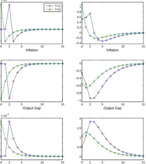
Figure 1 depicts impulse response functions of inflation, output gap, and price level in case of low (ω = 0.25, left column) and high (ω = 0.75, right col-umn) price rigidity under the optimal monetary policy with timeless perspective commitment. Solid lines with triangles denote responses to a cost-push shock that unexpectedly emerges in period t = 0, solid lines with circles denote re-sponses to a cost-push shock whose realization in periodT = 2 is anticipated in periodt= 0.
We firstly consider the empirically plausible case of high price rigidity. In case of an unanticipated cost-shock, both the price level and inflation rise whereas output falls in response to the realization of the increase in the costs of production.3 Subsequently, all variables converge in a hump-shaped fashion to their respective steady state values.
Anticipated cost shocks have two effects, namely the anticipation effect which reflects the change in xt, πt, and pt in response to the anticipation of
a future change in costs, and the realization effect which occurs when the an-ticipated change in costs actually takes place. Under the optimal monetary policy with commitment, output starts to decline and prices begin to increase in response to the anticipation of a future rise in the costs of production. Both
3
We could think about this cost-push shock as an exogenous rise in wage mark-ups (see, for example, Gal´ı (2008)).
0 2 5 10 15 −5
0 5 10
x 10−3 LOW PRICE RIGIDITY
Inflation 0 2 5 10 15 −0.15 −0.1 −0.05 0 Output Gap 0 2 5 10 15 0 2 4 6 8 10 x 10−3 Price Level 0 2 5 10 15 −0.4 −0.2 0 0.2 0.4 0.6 0.8 1
HIGH PRICE RIGIDITY
Inflation 0 2 5 10 15 −1 −0.8 −0.6 −0.4 −0.2 0 Output Gap 0 2 5 10 15 0 0.5 1 1.5 2 Price Level T=2 T=0
Figure 1: Impulse response functions under optimal policy with timeless perspective commitment.
Notes: Solid lines with triangles denote responses to an unanticipated cost-push shock, solid lines with circles denote responses to an anticipated cost-push shock. In case of low price rigidity, the Calvo parameter ω is set to 0.25; in case of high price rigidity,ωis set to 0.75.
variables respond in a hump-shaped fashion peaking at the date of realization. The increase in prices causes inflation to jump at the time of anticipation, peak-ing at the date of realization and then returnpeak-ing in a hump-shaped fashion to its initial steady state level.
In case oflow price rigidity, an unanticipated cost shock causes an immediate rise in prices and an immediate drop in output. Subsequently, both variables converge monotonically to their initial steady state levels. After the initial
jump, inflation falls sharply and converges from below to its pre-shock level. The announcement of a future rise in costs has negligible anticipation effects when prices are highly flexible. The reason is that the price setting problem of firms becomes more of an atemporal (static) nature when the Calvo parameter
ω decreases. In this case firms know that, with a high probability, they will be able to raise their price when the anticipated shock actually materializes in period T. Thus, output and prices change only slightly in response to an announcement or anticipation of future cost-push shocks.
Regardless of the degree of price rigidity, Figure 1 illustrates that the initial jumps of inflation, output gap and price level are greater in case of unantic-ipated (T = 0) than in case of anticipated shocks (T = 2). On the other hand, anticipated shocks amplify the persistence ofpt, xt, andπt compared to
unanticipated shocks.4 0 5 10 15 20 25 30 0.0145 0.0145 0.0145 0.0145 0.0145 0.0145 0.0145 0.0145 0.0145 Total Loss LOW PRICE RIGIDITY
0 5 10 15 20 25 30 2 2.5 3 3.5 4 Total Loss HIGH PRICE RIGIDITY
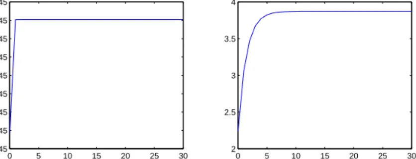
Figure 2: Welfare loss for different lengths of anticipation period under op-timal timeless perspective commitment policy in caseβ= 1.
Figure 2 illustrates the welfare lossV =V(T) in case β= 1. Without time discounting in the intertemporal loss function, the persistence effect always dominates the anticipation effect so that proposition 1 holds. In Figure 2, the total lossV =V(T) is overall increasing inT ifβ= 1.
If future deviations of the state variables from their initial steady state levels are discounted, the contribution of the initial jumps of output and inflation for the determination of the total loss becomes more important. The same holds for increasing degree of price flexibility 1−ω, since the persistence of prices, output and inflation is a decreasing function of 1−ω. If the degree of price flexibility is high, the value of the total loss is almost completely determined by the size of the initial jumps of xt and πt which in turn is inversely proportional to the
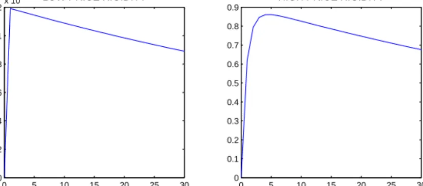
lead time T. With a sufficiently high degree of price flexibility, the total loss under unanticipated cost-push shocks is greater than the loss under anticipated shocks so that proposition 3 holds. This result is also illustrated in Figure 3, where V(T) is a monotonically decreasing function in the lead time T if the degree of price rigidity ω is very small.
4
This result also holds in the special caseϕ= 0, i.e. if the shock exhibits no serial correlation. It is well-known that even in this case the optimal precommitment policy introduces inertia in the impulse response functions.
0 5 10 15 20 25 30 0.0105 0.011 0.0115 0.012 0.0125 0.013 0.0135 0.014 0.0145 Total Loss LOW PRICE RIGIDITY
0 5 10 15 20 25 30 2 2.5 3 3.5 Total Loss HIGH PRICE RIGIDITY
Figure 3: Welfare loss for different lengths of anticipation period under op-timal timeless perspective commitment policy in caseβ= 0.99.
From an empirical point of view, the parameterω is not that small so that the development of the impulse response functions displays inertia or strong serial correlation. Then, if the time span between the anticipation and the implementation of the cost-push shock is not too long, the persistence effect dominates and the value of the total loss V(T) is greater than V(0). This is illustrated in Figure 3, where the development of the loss function V(T) is hump-shaped and monotonically increasing for small values ofT.
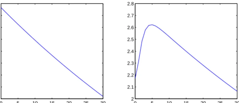
Propositions 1 to 3 are independent of the chosen optimal monetary policy regime. They hold under timeless perspective commitment as well as under discretion (see Figure 4 and 5 for a numerical visualization). They also hold under simple monetary policy rules (such as Taylor-type rules or money growth peg). 0 5 10 15 20 25 30 0.0146 0.0146 0.0146 0.0146 0.0146 0.0146 0.0146 0.0146 0.0146 Total Loss LOW PRICE RIGIDITY
0 5 10 15 20 25 30 2 4 6 8 10 12 14 16 Total Loss HIGH PRICE RIGIDITY
Figure 4: Welfare loss for different lengths of anticipation period under the optimal discretionary policy in caseβ= 1.
In order to check whether the welfare-reducing effects of anticipations hold for empirically plausible degrees of nominal rigidity, we compute the critical anticipation valuesT∗
c (commitment) andTd∗ (discretion). Table 1 depicts the
values of T∗
c and Td∗ for a persistent (ϕ = 0.5) and a one-off cost-push shock
(ϕ= 0).
Table 1 shows that the anticipation of cost-push shocks dampens the welfare loss induced by such shocks only for empirically unrealistic degrees of nominal
0 5 10 15 20 25 30 0.0105 0.011 0.0115 0.012 0.0125 0.013 0.0135 0.014 0.0145 Total Loss LOW PRICE RIGIDITY
0 5 10 15 20 25 30 3 4 5 6 7 8 9 10 11 12 Total Loss HIGH PRICE RIGIDITY
Figure 5: Welfare loss for different lengths of anticipation period under the optimal discretionary policy in caseβ= 0.99.
rigidity. For the widely applied values ofω= 0.75 orω = 0.66, the anticipation period or lead time T must be extremely large to obtain a welfare gain from anticipation. Under commitment and a value ω = 0.75, the loss under an anticipated shock is smaller than the loss under an unanticipated shock of same size when the shock is anticipated to take place in T∗
c = 54 (for ϕ = 0.5) or
T∗
c = 66 (for ϕ = 0) quarters. Even larger values are obtained under optimal
discretionary policy. A Calvo parameter of 0.5 represents the lower bound in the range of values that are reported in the literature. In this case and under the monetary policy regime commitment, the anticipation of future cost shocks has a welfare-enhancing effect if the lead time is larger or equal to two quarters for persistent and three quarters for one-off shocks, respectively. Under discretionary monetary policy, these critical values are three and four quarters. Our simulations illustrate that for a wide range of empirically realistic de-grees of nominal rigidities (i.e.,ω≥0.5) in conjunction with a plausible length of the anticipation period, the welfare loss of anticipated cost shocks exceeds the welfare loss of unanticipated cost shocks.
Table 1: Values of the critical lead time T∗
c andTd∗
Degree of price rigidity ω
Monetary policy 0.75 0.66 0.60 0.55 0.50 0.45 0.40 0.25 Withϕ= 0.5 Commitment 53.09 19.82 9.00 4.23 1.82 0.69 0.16 0 Discretion 125.90 40.41 15.61 6.37 2.42 0 0 0 Withϕ= 0 Commitment 65.78 25.57 11.79 5.59 2.41 0.95 0.28 0 Discretion 146.99 50.77 20.25 8.38 3.20 0 0 0
Note: For an anticipation period 0< T < Ti∗it is true thatV|T > V|T=0, forT > Ti∗ it is
4
Conclusion
In this paper we investigate the welfare effects resulting from the anticipation of future shocks. In particular, we analyze the welfare loss for different lengths of the time span between the anticipation and the realization of cost-push shocks. This includes the widely applied case of unanticipated cost-push shocks. Our analysis is based on the canonical New Keynesian model with optimal monetary policy.
We emphasize the role of nominal rigidities for the welfare effects of an-ticipations. We show that for empirically plausible degrees of nominal rigidity, anticipated cost shocks entail higher welfare losses than unexpected cost shocks. The anticipation of a future cost-push shock dampens the volatility of output and inflation only if prices are highly flexible. These results hold independently of the monetary policy regime (timeless perspective commitment, discretion, (optimal) simple rules).
Our results imply that the knowledge about the realization of future cost shocks is in general welfare-reducing. The question remains why rational agents do not simply ignore this information. However, this would be inconsistent with the profit-maximizing behavior of individual firms and the utility-maximizing behavior of individual households on which our model is based. The firm’s optimality condition in fact calls for an increase in prices in response to the anticipation of a future rise in costs. By simply ignoring this information, the firm would make a loss.
Hence, our results reveal a contradiction between the optimal behavior of individuals and the optimum from a social point of view.
References
Ball, L. (1994). Credible Disinflation with Staggered Price Setting. American Economic Review 84, 282–289.
Beaudry, P., Portier. F. (2004). An Exploration into Pigou’s Theory of Cycles.
Journal of Monetary Economics 51, 1183–1216.
Beaudry, P., Portier. F. (2006). Stock Prices, News, and Economic Fluctuations.
American Economic Review 96, 1293–1307.
Beaudry, P., Portier. F. (2007). When Can Changes in Expectations Cause Business Cycle Fluctuations in Neo-Classical Settings? Journal of Economic Theory 135, 458–477.
Beaudry, P., Collard, F., Portier. F. (2006). Gold Rush Fever in Business Cycles. NBER Working Paper 12710. National Bureau of Economic Research. Blanchard, O. J., Kahn, K. (1980). The Solution of Linear Difference Models
under Rational Expectations.Econometrica 48, 1305–1311.
Calvo, G. (1983). Staggered Prices in a Utility Maximizing Framework.Journal of Monetary Economics 12, 383–398.
Christiano, L. J., Eichenbaum, M., Evans, C. L. (2005). Nominal Rigidities and the Dynamic Effects of a Shock to Monetary Policy. Journal of Political Economy 113, 1–45.
Christiano, L. J., Ilut, C., Motto, R., Rostagno, M. (2008). Monetary Policy and Stock Market Boom-Bust Cycles. ECB Working Paper 955. European Central Bank.
Clarida, R. H., Gal´ı, J., Gertler, M. (1999). The Science of Monetary Policy: A New Keynesian Perspective. Journal of Economic Literature 37, 1661–1707. Davis, J. M. (2007). News and the Term Structure in General Equilibrium.
Unpublished Manuscript.
Den Haan, W. J., Kaltenbrunner, G. (2007). Anticipated Growth and Busi-ness Cycles in Matching Models. CEPR Discussion Papers 6063. Centre for Economic Policy Research.
Fujiwara, I., Hirose, Y., Shintani, M. (2008). Can News Be a Major Source of Aggregate Fluctuations? A Bayesian DSGE Approach. IMES Discussion Pa-per 2008-E-16. Institute for Monetary and Economic Studies, Bank of Japan. Gal´ı, J. (2008). Monetary Policy, Inflation, and the Business Cycle. Princeton
University Press.
Khan, A., King, R. G., Wolman, A. L. (2003). Optimal Monetary Policy.Review of Economic Studies 70, 825–860.
Kydland, F. E., Prescott, E. C. (1982). Time to Build and Aggregate Fluctua-tions. Econometrica 50, 1345–1370.
Jaimovich, N., Rebelo, S. (2006). Can News About the Future Drive the Busi-ness Cycle? NBER Working Paper 12537. National Bureau of Economic Research.
Jaimovich, N., Rebelo, S. (2008). News and Business Cycles in Open Economies.
Journal of Money, Credit and Banking 40, 1699–1711.
Rotemberg, J. J., Woodford, M. (1999). Interest Rate Rules in an Estimated Sticky Price Model. In: Taylor, J. B. (Ed.),Monetary Policy Rules, University of Chicago Press, 57–119
Schmitt-Groh´e, S., Uribe, M. (2007). Incomplete Cost Pass-Through under Deep Habits. NBER Working Paper 12961. National Bureau of Economic Research.
Schmitt-Groh´e, S., Uribe, M. (2008). What’s News in Business Cycles. NBER Working Paper 14215, National Bureau of Economic Research.
Svensson, L. E. O. (1999). Inflation Targeting as a Monetary Policy Rule. Jour-nal of Monetary Economics 43, 607–654.
Walsh, C. E. (2003).Monetary Theory and Policy. Second Edition. MIT Press. Winkler, R. (2008). Oil Price Shocks, Ramsey Monetary Policy, and Welfare.
Unpublished Manuscript, Christian-Albrechts-Universit¨at Kiel.
Wohltmann, H.-W., Winkler, R. (2008a). Anticipated and Unanticipated Oil Price Shocks and Optimal Monetary Policy. Economics Working Paper 2008-05. Department of Economics, Christian-Albrechts-Universit¨at Kiel.
Woodford, M. (2003). Interest and Prices: Foundations of a Theory of Mone-tary Policy. Princeton University Press.
Mathematical Appendix
Solution time paths under the optimal timeless perspective pre-commitment policy
It is well-known that under the optimal timeless perspective precommitment policy inflation and the output gap satisfy
πt=− α2 α1κ (xt−xt−1) (1) and 1 +β+ α1κ 2 α2 xt−xt−1−βEtxt+1 =−α1κ α2 kt (2)
where the expectational operator can be omitted in case of anticipated shocks. To solve the difference equation forxt write equation (2) as
xt+1 wt+1 =C xt wt + α1κ α2β 0 kt (3) wherewt=xt−1 and C= 1 β 1 +β+α1κ2 α2 −β1 1 0 ! (4)
The auxiliary variable wt is backward-looking (with the initial value w0 = 0)
while the output gapxt is forward-looking. The system matrixC has two real
eigenvaluesr1 and r2 withr1 >1> r2 >0 so that the Blanchard/Kahn (1980)
saddlepath stability condition is satisfied. The eigenvalues are given by
r1,2 = 1 2trC± r 1 2(trC)2− |C| (5) with trC= 1 β 1 +β+α1κ 2 α2 =r1+r2, |C|= 1 β =r1r2 (6)
We can transfer system (3) into Jordan-canonical form using the similarity transformation
C =H·Λ·H−1 (7)
where Λ = diag(r1, r2) is a diagonal matrix whose diagonal elements are the
characteristic roots ofC and
H= r1 r2 1 1 (8)
is a matrix of linearly independent eigenvectors ofC. Define auxiliary variables vtand zt by H−1 xt wt = vt zt or xt wt =H vt zt (9) Premultiplying equation (3) withH−1 yields the Jordan-canonical system
vt+1 zt+1 = r1 0 0 r2 vt zt + 1 r1−r2 α1κ α2β 1 −1 kt (10)
The difference equation in vt contains the unstable eigenvalue r1 and has the
unique stable forward solution
vt=− ∞ X s=0 r1−s1 r1 1 r1−r2 α1κ α2β kt+s (11)
Since the cost-push shockkt+s is a AR(1) variable with
kt+s= ( ϕt+s−T for t+s≥T 0 for t+s < T (12) we obtain vt= − 1 r1−ϕ 1 r1−r2 α1κ α2β ϕt−T for t≥T − 1 r1−ϕ 1 r1−r2 α1κ α2β rt1−T for t≤T (13)
with the initial value
v0 =− 1 r1−ϕ 1 r1−r2 α1κ α2β r1−T <0 (14) The difference equation inzt has the general backward solution
zt=r2tK− t−1 X s=0 r2t−s−1 1 r1−r2 α1κ α2β ks (15)
where the constantK follows from the initial condition
z0=K=w0−v0 =−v0 (16)
Sinceks= 0 for s < T we obtain
zt=r2tK = 1 r1−ϕ 1 r1−r2 α1κ α2β r1−Trt2 fort≤T (17) and zt=r2tK− 1 r2−ϕ 1 r1−r2 α1κ α2β h rt2−T −ϕt−Ti (18) = 1 r1−r2 α1κ α2β " r−1T r1−ϕ − r −T 2 r2−ϕ ! r2t+ ϕ −T r2−ϕ ϕt # for t≥T
The solution for the output gapxt=r1vt+r2zt is then given by xt=− 1 r1−ϕ 1 r1−r2 α1κ α2β r1−T(r1t+1−rt2+1) for t≤T (19) with the initial values
x0 =− 1 r1−ϕ α1κ α2β r1−T , x−1 = 0 (20) and xt= α1κ α2β 1 (r1−ϕ)(r2−ϕ) · (21) · " ϕt+1−T −(r1−ϕ)r2−T −(r2−ϕ)r1−T r1−r2 rt2+1 # fort≥T
The solution formula (21) also contains the limiting case T = 0, i.e., if the cost-push shock is not anticipated. The term in brackets then simplifies to
ϕt+1−rt+1 2 .
Using (1), the solution time path of the inflation rate follows:
πt= 1 β 1 r1−ϕ 1 r1−r2 r1−T (r1−1)rt1−(r2−1)r2t fort≤T (22) with the initial value
π0 = 1 β 1 r1−ϕ r1−T (23) and πt= 1 β 1 r1−ϕ 1 r2−ϕ · (24) · " (1−ϕ)ϕt−T −(r1−ϕ)r −T 2 −(r2−ϕ)r−1T r1−r2 (1−r2)r2t # fort≥T
In the special caseT = 0 the term in brackets simplifies to (1−ϕ)ϕt−(1−r 2)r2t.
The solution time path of the price levelptcan be derived from the solution
ofπtdue to pt= t X k=0 πk (25)
We then obtain for ort≤T:
pt= 1 β 1 r1−ϕ 1 r1−r2 r1−T t X k=0 h (r1−1)r1k−(r2−1)r2k i (26) =1 β 1 r1−ϕ 1 r1−r2 r1−T (r1−1) 1−rt1+1 1−r1 −(r2−1) 1−r2t+1 1−r2 =1 β 1 r1−ϕ 1 r1−r2 r1−T r1t+1−rt2+1
and fort≥T pt= T−1 X k=0 πk+ t X k=T πk (27) = 1 β 1 r1−ϕ 1 r1−r2 r1−T rT1 −r2T + 1 β 1 r1−ϕ 1 r2−ϕ · · t X k=T ( (1−ϕ)ϕk−T −(r1−ϕ)r −T 2 −(r2−ϕ)r−1T r1−r2 (1−r2)rk2 ) = 1 β 1 r1−ϕ 1 r1−r2 r1−T rT1 −r2T + 1 β 1 r1−ϕ 1 r2−ϕ · · " −(1−ϕ)ϕ−Tϕ t+1−ϕT 1−ϕ + (r1−ϕ)r2−T −(r2−ϕ)r−1T r1−r2 (1−r2) r2t+1−rT 2 1−r2 # = 1 β 1 r1−ϕ 1 r1−r2 r1−T rT1 −r2T + 1 β 1 r1−ϕ 1 r2−ϕ · · " 1−ϕt+1−T +(r1−ϕ)r −T 2 −(r2−ϕ)r−1T r1−r2 rt2+1−r2T # = 1 β 1 r2−ϕ 1 r1−r2 r2t+1−T − 1 β 1 r1−ϕ 1 r1−r2 r−1Tr2t+1− 1 β 1 r1−ϕ 1 r2−ϕ ϕt+1−T Obviously, lim t→∞pt= 0 for all T ≥0 (28) and p0= 1 β 1 r1−ϕ r−1T =π0 >0 (29)
so that the size of the initial jump inpis inversely proportional to the lead time
T.
Similar results hold for the state variables xt and πt. Since t X k=0 (xk−xk−1) =xt (30) equation (1) implies pt= t X k=0 πk=− α2 α1κ t X k=0 (xk−xk−1) =− α2 α1κxt (31)
so thatpt>0 if and only ifxt<0. The optimal policy under timeless
perspec-tive impliespt>0 for all 0≤t <∞ so that xt<0 for all t <∞. We can also
show that thepersistence ortotal variation of pt is positive correlated withT,
i.e. ∞ X t=0 pt T =0 < ∞ X t=0 pt T > 0 for all T >0 (32)
where the infinite sumP∞ t=0pt T >0 is an increasing function in T.
The persistence measure used here is based on the deviation ofpt from its
initial steady state levelp0, where the deviation|pt−p0|is calculated both for
t < T and t ≥ T. Thereafter the differences |pt−p0| are summed up. Since
p0= 0 and pt>0 for all twe must determine the infinite sum P∞t=0pt.
Inequality (32) holds although the initial jump of pt is a negative function
inT. To prove the inequality note that ∞ X t=0 pt T=0 = 1 β(r1−ϕ)(r2−ϕ) r2 1−r2 − ϕ 1−ϕ (33) = 1 β(r1−ϕ)(1−r2)(1−ϕ) T X t=0 pt T >0 = 1 β(r1−ϕ)(r1−r2) r−1T " r1 1−r1T+1 1−r1 −r2 1−r2T+1 1−r2 # (34) and ∞ X t=T+1 pt T >0 = 1 β(r2−ϕ)(r1−r2) r12−T r T+1 2 1−r2 (35) − 1 β(r1−ϕ)(r1−r2) r1−Tr2 rT2+1 1−r2 − 1 β(r1−ϕ)(r2−ϕ) ϕ1−T ϕ T+1 1−ϕ so that ∞ X t=0 pt T >0 = 1 β(r1−ϕ)(r1−r2) r11−T 1−r1 − r 2 1 1−r1 − r2r −T 1 1−r2 (36) +r −T 1 r2T+2 1−r2 − r −T 1 rT2+2 1−r2 + 1 β(r2−ϕ) 1 r1−r2 r22 1−r2 − 1 r1−ϕ ϕ2 1−ϕ = 1 β(r1−ϕ)(r1−r2) " r1 1−r1 r−1T −r1 −r2r −T 1 1−r2 # + 1 β(r2−ϕ) 1 r1−r2 r2 2 1−r2 − 1 r1−ϕ ϕ2 1−ϕ
Then ∞ X t=0 pt T >0> ∞ X t=0 pt T=0 ⇔ (37) 1 β(r1−ϕ)(r1−r2) r1 1−r1 r1−T −r1 − r2 1−r2 1 β(r1−ϕ)(r1−r2) r−1T − 1 β(r2−ϕ) r2 r1−r2 + 1 β(r1−ϕ)(r2−ϕ) − 1 β(r2−ϕ) 1 r1−ϕ ϕ 1−ϕ[ϕ−1]>0 ⇔ 1 β(r1−ϕ)(r1−r2) r1 1−r1 r−1T −r1 − 1 β(r1−ϕ)(r1−r2) r2 1−r2 r−1T −r1 − 1 β(r1−ϕ)(r1−r2) r2 1−r2 r1 − r2 1−r2 − r1−ϕ β(r1−ϕ)(r2−ϕ) r2 r1−r2 + r1−r2 β(r1−ϕ)(r2−ϕ)(r1−r2) + 1 β(r1−ϕ)(r2−ϕ) ϕ >0 ⇔ 1 β(r1−ϕ)(r1−r2) r1−T −r1 r1 1−r1 − r2 1−r2 + r2 1−r2 1 β(r1−ϕ)(r2−ϕ)(r1−r2) · ·[r2(r1−ϕ)−(r1−r2)−(r2−ϕ)r1] + 1 β(r1−ϕ)(r2−ϕ) ϕ >0 ⇔ 1 β(r1−ϕ)(r1−1)(1−r2) r1−r−1T + 1 β(r1−ϕ)(r2−ϕ) · · ϕ+ r2 (1−r2)(r1−r2) (r2(r1−ϕ)−(r1−r2)−(r2−ϕ)r1) >0 ⇔ 1 β(r1−ϕ)(r1−1)(1−r2) r1−r1−T + 1 β(r1−ϕ)(r2−ϕ) (r1−r2)(ϕ−r2) (1−r2)(r1−r2) >0 ⇔ 1 β(r1−ϕ)(r1−1)(1−r2) r1−r1−T − 1 β(r1−ϕ)(1−r2) >0 ⇔ r1−r1−T −(r1−1) >0 ⇔ 1−r−1T >0 Since r1 > 1 the last inequality is fulfilled. Note that the total variation of
pt, i.e. P∞t=0pt
T >0 is an increasing function in T. This follows from equation
(36), since the derivative of r1
1−r1r −T 1 − r 2 1−r2r −T
An implication of inequality (37) is ∞ X t=0 |xt| T =0 < ∞ X t=0 |xt| T > 0 (38) since |xt|= α1κ α2 pt (39)
The persistence of the output response in case of anticipated cost-push shocks is therefore stronger than in case of unanticipated shocks.
A similar result can be shown for the inflation rate πt if the limiting case
ϕ= 0 is considered. We then get for T = 0
πt= ( 1−(1−r2) =r2 if t= 0 −(1−r2)rt2<0 if t >0 (40) implying ∞ X t=0 πt=π0+ ∞ X t=1 πt=r2−(1−r2) ∞ X t=1 rt2 (41) =r2−(1−r2) 1 1−r2 −1 =r2−r2 = 0 and ∞ X t=0 |πt| T=ϕ=0 =r2+ (1−r2) ∞ X t=1 rt2= 2r2 (42)
In caseT >0 and ϕ= 0 we get - fort≤T: πt= r2 r1−r2 r−1T (r1−1)r1t−(r2−1)r2t >0 (43) - fort > T: πt=− r1r2−T −r2r1−T r1−r2 (1−r2)r2t <0 (44) Then T X t=0 πt= r2 r1−r2 r−1T T X t=0 (r1−1)r1t−(r2−1)r2t (45) = r2 r1−r2 r−1T " (r1−1) 1−rT1+1 1−r1 + (1−r2) 1−r2T+1 1−r2 # = r2 r1−r2 r−1T hrT1+1−rT2+1i
and ∞ X t=T+1 πt=− 1−r2 r1−r2 h r1r2−T −r2r1−T i rT+1 2 1−r2 (46) =− r2 r1−r2 r1−Thr1T+1−r2T+1i so that ∞ X t=0 πt= 0 (47) and ∞ X t=0 |πt| T >0 ϕ=0 = 2 r2 r1−r2r −T 1 h r1T+1−r2T+1i (48) Now r2 r1−r2 r−1ThrT1+1−rT2+1i> r2 ⇔ (49) r−1ThrT1+1−rT2+1i> r1−r2 ⇔ r1T+1−r2T+1> r1T+1−r2r1T ⇔ r2r1T −r2T+1>0 ⇔ r2 r1T −rT2 >0
Due tor1 >1> r2>0 the last inequality is met so that
∞ X t=0 |πt| T=ϕ=0 < ∞ X t=0 |πt| T >0 ϕ=0 (50)
The caseϕ >0 is more difficult to analyze since πt can take both positive and
negative values for t > T >0. IfT = 0, πt changes sign immediately after the
initial jump. Since
πt= 1 β(r1−ϕ)(r2−ϕ) (1−ϕ)ϕt−(1−r2)rt2 (ifT = 0) (51) we get π0= 1 β(r1−ϕ) >0 (52) and ∞ X t=1 πt T=0 = 1 β(r1−ϕ)(r2−ϕ) " (1−ϕ) ∞ X t=1 ϕt−(1−r2) ∞ X t=1 r2t # (53) = 1 β(r1−ϕ)(r2−ϕ) (1−ϕ) 1 1−ϕ−1 −(1−r2) 1 1−r2 −1 = 1 β(r1−ϕ)(r2−ϕ) (ϕ−r2) =− 1 β(r1−ϕ) =−π0
so that ∞ X t=0 |πt| T=0 = 2 1 β(r1−ϕ) (54)
In caseT >0 πt is positive for 0≤t≤T and we obtain due to (22) T X t=0 πt= 1 β(r1−ϕ)(r1−r2) r1−T " (r1−1) 1−rT1+1 1−r1 −(r2−1) 1−rT2+1 1−r2 # (55) = 1 β(r1−ϕ)(r1−r2) r1−Th−1−r1T+1+ 1−rT2+1i = 1 β(r1−ϕ)(r1−r2) r1−ThrT1+1−rT2+1i = r1 β(r1−ϕ)(r1−r2) " 1− r2 r1 T+1# >0
(sincer1 >1> r2 >0). If t > T, πt is negative for sufficiently large values of
t. For small values oft > T πt may be positive. Due to
lim t→∞pt= 0 and pt= t X k=0 πk (56) we must have ∞ X t=0 πt= 0 (57) so that ∞ X t=T+1 πt=− T X t=0 πt<0 (58)
The last equation also follows from (24): With
ψ=−(r1−ϕ)r
−T
2 −(r2−ϕ)r1−T
r1−r2
we obtain ∞ X t=T+1 πt= 1 β(r1−ϕ)(r2−ϕ) " (1−ϕ)ϕ−T ∞ X t=T+1 ϕt+ψ(1−r2) ∞ X t=T+1 r2t # (60) = 1 β(r1−ϕ)(r2−ϕ) " (1−ϕ)ϕ−T ϕ T+1 1−ϕ+ψ(1−r2) r2T+1 1−r2 # = 1 β(r1−ϕ)(r2−ϕ) h ϕ+ψr2T+1i = 1 β(r1−ϕ)(r2−ϕ) " ϕ−(r1−ϕ)r −T 2 −(r2−ϕ)r−1T r1−r2 r2T+1 # = 1 β(r1−ϕ)(r2−ϕ) ϕ− r1−ϕ r1−r2 r2+ r2−ϕ r1−r2 r1−TrT2+1 = 1 β(r1−ϕ)(r2−ϕ)(r1−r2) h ϕ(r1−r2)−r2(r1−ϕ) + (r2−ϕ)r1−TrT2+1 i = 1 β(r1−ϕ)(r2−ϕ)(r1−r2) h (ϕ−r2)r1+ (r2−ϕ)r−1TrT2+1 i = 1 β(r1−ϕ)(r1−r2) h −r1+r1−TrT2+1 i =− r1 β(r1−ϕ)(r1−r2) " 1− r2 r1 T+1# =− T X t=0 πt<0 Therefore, T X t=0 πt T >0− ∞ X t=T+1 πt T >0 = 2 T X t=0 πt T >0 > ∞ X t=0 |πt| T=0= 2π0 T=0 ⇔ (61) T X t=0 πt T >0 > π0 T=0 ⇔ r1 β(r1−ϕ)(r1−r2) 1−(r2 r1 )T+1 > 1 β(r1−ϕ) ⇔ r1 r1−r2 " 1− r2 r1 T+1# >1 ⇔ r1 " 1− r2 r1 T+1# > r1−r2 ⇔ r2 > r1 r2 r1 T+1 ⇔ 1> r2 r1 T ⇔ rT1 > rT2
The last inequality is met due tor1>1> r2 >0. Since − ∞ X t=T+1 πt T > 0≤ ∞ X t=T+1 |πt| T > 0 (62)
the stronger persistence in case of anticipated shocks follows: ∞ X t=0 |πt| T >0 = T X t=0 πt+ ∞ X t=T+1 |πt| ≥ T X t=0 πt− ∞ X t=T+1 πt> ∞ X t=0 |πt| T=0 (63)
Note that for arbitraryT >0
π0 T=0 < T X t=0 πt T >0 (64) but πt T >0 < π0 T=0 for all 0≤t≤T (65) In particular πT T >0< π0 T=0 (66) since πt T >0= 1 β(r1−ϕ)(r1−r2) r1−T (r1−1)rT1 −(r2−1)r2T (67) = 1 β(r1−ϕ)(r1−r2) " (r1−1)−(r2−1) r2 r1 T# < π0 T=0 = 1 β(r1−ϕ) ⇔ 1 r1−r2 " (r1−1)−(r2−1) r2 r1 T# <1 ⇔ (r1−1)−(r2−1) r2 r1 T < r1−r2 ⇔ (1−r2) r2 r1 T <1−r2 ⇔ r2 r1 T <1
Since the last equation holds, the value of the inflation rate at the time of implementation of the cost-push shock is smaller in case of anticipated compared to unanticipated shocks.5
5
This result holds under the optimal timeless perspective precommitment policy. Under the policy regime discretion we have (cf. (138))
π0 T=0 =πT T >0 = α2 α2+α1κ2−α2βϕ
The loss under the optimal policy
To determine the welfare loss under the optimal precommitment policy, write the loss functionV asV1+V2, where
V1 =E0 T−1 X t=0 βt α1πt2+α2x2t (68)
is the loss resulting from the anticipation of the shock and
V2=E0 ∞ X t=T βt α1πt2+α2x2t (69)
is the loss following from the realization of the shock. We first calculate the value of the loss function V1. Since the solution time path of the state vector
(πt, xt)′ over the anticipation interval can be written as
πt xt =G rt 1 0 0 rt 2 1 1 (t < T) (70) where G= (r1−1)r− T 1 β(r1−ϕ)(r1−r2) −(r2−1)r− T 1 β(r1−ϕ)(r1−r2) −α1κ α2β r1−T 1 (r1−ϕ)(r1−r2) α1κ α2β r2r− T 1 (r1−ϕ)(r1−r2) (71) we obtain V1 = T−1 X t=0 βt πt xt ′ α1 0 0 α2 πt xt (72) = T−1 X t=0 βt 1 1 ′ rt 1 0 0 rt 2 G′ α1 0 0 α2 G rt 1 0 0 rt 2 1 1 = 1 1 ′ W1 1 1 = tr W1 1 1 1 1 ′ =w(1)11 + 2w(1)12 +w22(1)
where the symmetric matrixW1 =
w(1)ij
1≤i,j≤2 is defined as the finite sum of
matrices W1= T−1 X t=0 βt rt 1 0 0 rt 2 D rt 1 0 0 rt 2 (73) with D= d11 d12 d12 d22 =G′ α1 0 0 α2 G (74)
The elements of the symmetric matrixDare given by d11=α1λ2r1−2T (r1−1)2+ α1κ2 α2 r21 (75) d12=−α1λ2r1−2T (r1−1)(r2−1) + α1κ2 α2 r1r2 (76) d22=α1λ2r1−2T (r2−1)2+ α1κ2 α2 r22 (77) where we have used the abbreviation
λ= 1 β 1 r1−ϕ 1 r1−r2 (78) According to (6) we have (r1−1)(r2−1) +α1κ 2 α2 r1r2= (79) r1r2 1 + α1κ 2 α2 + 1−(r1+r2) = 1 β 1 + α1κ 2 α2 + 1−(r1+r2) = trC−1 + 1−(r1+r2) = 0 so that w(1)11 =d11 T−1 X t=0 βtr21t= 1−β Tr2T 1 1−βr21 d11 (80) w(1)12 =d12 T−1 X t=0 βtrt1r2t = 0 (81) w(1)22 =d22 T−1 X t=0 βtr22t= 1−β Tr2T 2 1−βr2 2 d22 (82) Using (6) we get (r1−1)2+ α1κ2 α2 r12= (83) r21 1 + α1κ 2 α2 + 1−2r1 = β r12[r1+r2−1] + 1 β[1−2r1] = 1 r2 r1[r1+r2−1] +r2[1−2r1] = 1 r2 (r1−r2)(r1−1)
so that w11(1)= r T 2 −rT1 (r2−r1)r2T−1 α1λ2r1−2T 1 r2(r1−r2)(r1−1) (84) =α1λ2r1−2T rT 1 −rT2 rT 2 (r1−1) and analogically w22(1)=α1λ2r1−2T rT 1 −rT2 rT 1 (1−r2) (85)
Then the loss V1 can be written as
V1 =α1λ2r1−2T r1T −rT2 r1−1 rT 2 + 1−r2 rT 1 (86)
ConsiderV1 as function inT (the time span between the anticipation and
real-ization of the cost-push shock). The functionV1(T) has the following properties:
V1(0) = 0, lim T→∞V1(T) = ( 0 forβ <1 V1>0 forβ = 1 (87) where V1= α1(r1−1) (r1−ϕ)2(r1−r2)2 (88) The derivative ofV1 with respect toT, i. e.
dV1 dT =α1λ 2 2 lnr1·r1−2T[r1+r2−2]−(r1−1) ln(r1r2)·(r1r2)−T (89) −(1−r2) ln( r2 r3 1 )·(r2 r3 1 )T is positive at timeT = 0: dV1 dT T=0=α1λ 2 2(lnr1)(r1+r2−2) (90) −(r1−1) ln(r1r2)−(1−r2) ln r2 r3 1 =α1λ2(r1−r2)[lnr1−lnr2] =α1 1 β2 1 (r1−ϕ)2 1 r1−r2 [lnr1−lnr2]>0
Therefore,V1(T) starts to rise with increasingT (although the size of the initial
jumps of xt and πt is decreasing in T). For β < 1 the limit value is equal to
zero, thereforeV1(T) must decrease ifT is sufficiently large. Figure 6 illustrates
0 5 10 15 20 25 30 0 0.2 0.4 0.6 0.8 1 1.2x 10 −6
Loss in the Anticipation Phase LOW PRICE RIGIDITY
0 5 10 15 20 25 30 0 0.1 0.2 0.3 0.4 0.5 0.6 0.7 0.8 0.9
Loss in the Anticipation Phase HIGH PRICE RIGIDITY
Figure 6: Partial loss in the anticipation phase for different lengths of antic-ipation period under optimal timeless perspective commitment policy in case
β = 0.99.
To calculate the loss function V2, write (πt, xt)′ as
πt xt =F ϕt 0 0 rt 2 1 1 (t≥T) (91) where F = (1−ϕ)ϕ−T β(r1−ϕ)(r2−ϕ)
[
(r2−ϕ)r− T 1 −(r1−ϕ)r− T 2]
(1−r2) β(r1−ϕ)(r2−ϕ)(r1−r2) α1κ α2β ϕ−(T−1) (r1−ϕ)(r2−ϕ) α1κ α2β[
(r2−ϕ)r− T 1 −(r1−ϕ)r− T 2]
r2 β(r1−ϕ)(r2−ϕ)(r1−r2) (92) Then V2= ∞ X t=T βt πt xt ′ α1 0 0 α2 πt xt (93) = ∞ X t=T βt 1 1 ′ ϕt 0 0 rt 2 F′ α1 0 0 α2 F ϕt 0 0 rt 2 1 1 = 1 1 ′ W2 1 1 = tr W2 1 1 1 1 ′ =w11(2)+ 2w(2)12 +w(2)22where the symmetric matrixW2 =
wij(2)
1≤i,j≤2 is the geometric sum of
ma-trices W2= ∞ X t=T βt ϕ 0 0 r2 t Q ϕ 0 0 r2 t (94) with Q= q11 q12 q21 q22 =F′ α1 0 0 α2 F (95)
The elements of the symmetric matrixQare given by q11=α1δ2ϕ−2T (1−ϕ)2+α1κ 2 α2 ϕ2 (96) q12=α1δ2φϕ−T 1 r1−r2 (1−r2)(1−ϕ) + α1κ2 α2 r2ϕ (97) q22=α1δ2φ2 1 (r1−r2)2 (1−r2)2+ α1κ2 α2 r22 (98) with the abbreviations
δ= 1 β 1 r1−ϕ 1 r2−ϕ (99) and φ= (r2−ϕ)r−1T −(r1−ϕ)r2−T (100)
The definition ofW2 implies that the matrixW2 satisfies the matrix equation
W2 =βT ϕ 0 0 r2 T Q ϕ 0 0 r2 T + ∞ X t=T+1 βt ϕ 0 0 r2 t Q ϕ 0 0 r2 t (101) =βT ϕ 0 0 r2 T Q ϕ 0 0 r2 T + ∞ X t=T βt+1 ϕ 0 0 r2 t+1 Q ϕ 0 0 r2 t+1 =βT ϕ 0 0 r2 T Q ϕ 0 0 r2 T +β ϕ 0 0 r2 W2 ϕ 0 0 r2 Since βT ϕ 0 0 r2 T Q ϕ 0 0 r2 T = βTϕ2Tq 11 βTϕTr2Tq12 βTϕTrT 2q21 βTr22Tq22 (102) and W2−β ϕ 0 0 r2 W2 ϕ 0 0 r2 = (1−βϕ 2)w(2) 11 (1−βϕr2)w(2)12 (1−βϕr2)w(2)21 (1−βr22)w(2)22 ! (103) we obtain w11(2)= β Tϕ2T 1−βϕ2q11 (104) w12(2)=w21(2)= β TϕTrT 2 1−βϕr2 q12 (105)
w(2)22 = β
Tr2T 2
1−βr22q22 (106)
Using (6) and the definition ofqij we can write
w(2)11 =α1δ2 βT 1−βϕ2 (1−2ϕ) + 1 +α1κ 2 α2 ϕ2 (107) =α1δ2 βT r1r2−ϕ2 r1r2(1−2ϕ) + (r1+r2−1)ϕ2 w12(2)=α1δ2φ βTrT 2 1−βϕr2 1 r1−r2 (1−r2)(1−ϕ) + α1κ2 α2 r2ϕ (108) =α1δ2φ βTrT2 r1−ϕ 1 r1−r2 r1(1−r2)(1−ϕ) +r1r2 α1κ2 α2 ϕ =α1δ2φ βTrT 2 r1−ϕ 1 r1−r2 [r1(1−ϕ−r2) + (r1+r2−1)ϕ] =α1δ2φβTr2T 1−r2 r1−r2 w(2)22 =α1δ2φ2 β Tr2T 2 1−βr2 2 1 (r1−r2)2 (1−r2)2+ α1κ 2 α2 r22 (109) =α1δ2φ2βTr22T r1 r1−r2 1 (r1−r2)2 1−2r2+r22 1 + α1κ 2 α2 =α1δ2φ2βTr22T 1−r2 (r1−r2)2 Then V2 =α1δ2βT 1 r1r2−ϕ2 r1r2(1−2ϕ) + (r1+r2−1)ϕ2 (110) + 2φ r1−r2 r2T(1−r2) + φ2 (r1−r2)2 r22T(1−r2) Since 1 r1r2−ϕ2 r1r2(1−2ϕ) + (r1+r2−1)ϕ2= 1 + (r1+r2)ϕ−2r1r2 r1r2−ϕ2 ϕ (111) and (according to the definition ofφ)
1 + 1
r1−r2
φrT2 = 1 (r1−r2)rT1
we can write V2=α1δ2βT ( 1 + 1 r1−r2 φrT2 2 (1−r2) +r2+ (r1+r2)ϕ−2r1r2 r1r2−ϕ2 ϕ ) (113) =α1δ2βT 1 (r1−r2)2r12T (r2−ϕ)2 r2T −r1T 2 (1−r2) + r1(r2−ϕ)2 r1r2−ϕ2 = α1β T β2(r 1−ϕ)2 ( rT2 −rT12 (1−r2) (r1−r2)2r21T + r1 r1r2−ϕ2 )
The loss functionV2 =V2(T) has the following properties:
V2(0) = α1 β2(r 1−ϕ)2 r1 r1r2−ϕ2 >0 (114) lim T→∞V2(T) = 0 ifβ <1 V2> V2(0) β= 1 = α1r1 (r1−ϕ)2(1−ϕ2) ifβ = 1 (115) where V2= α1 (r1−ϕ)2 1−r2 (r1−r2)2 + r1 1−ϕ2 (116) The first derivative ofV2 with respect toT
dV2 dT = α1 β2(r 1−ϕ)2 βT ( r1 r1r2−ϕ2 lnβ (117) + 1−r2 (r1−r2)2 " (lnr2−3 lnr1) r2 r1 2T + 4 lnr1 r2 r1 T + lnβ #) implies forβ <1 dV2 dT T=0 = α1 β2(r 1−ϕ)2 r1 r1r2−ϕ2 lnβ <0 (118)
(since β = 1/(r1r2)). For β < 1, dV2/dT is also negative if T is sufficiently
large. Figure 7 illustrates that the development of V2 is overall decreasing if
the value of ω is sufficiently small (i.e., the degree of price flexibility is high); otherwise it is not monotone, but hump-shaped. For sufficiently large values of
ωthe loss functionV2has two extrema (a maximum and a minimum) which can
be determined from the first-order conditiondV2/dT = 0. The first extremum
of V2 cannot be represented graphically since the corresponding value of T is
very small. Note that in the limiting caseβ = 1 the loss function V2(T) is an
increasing function inT with a limit valueV2 > V2(0).
We can now derive the development of the total loss V = V1 +V2. We
0 5 10 15 20 25 30 0.0105 0.011 0.0115 0.012 0.0125 0.013 0.0135 0.014 0.0145
Loss in the Implementation Phase LOW PRICE RIGIDITY
0 5 10 15 20 25 30 2 2.1 2.2 2.3 2.4 2.5 2.6 2.7 2.8
Loss in the Implementation Phase HIGH PRICE RIGIDITY
Figure 7: Partial loss in the implementation phase for different lengths of anticipation period under optimal timeless perspective commitment policy in caseβ= 0.99.
limT→∞V(T) = 0. For small values ofω, i.e. a high degree of price flexibility, the total loss V is a decreasing function in T implying V(T) < V(0) for all
T >0. With high price flexibility the welfare loss under anticipated shocks is smaller than under unanticipated shocks. If ω is small, the persistence of the state variables is weak and the total loss is mainly determined by the size of the initial jumps ofxtand πtwhich is a decreasing function in T. By contrast,
for sufficiently large values ofω (i.e. a high degree of price rigidity) the jump variables xt and πt display a strong persistence so that the welfare loss starts
to rise with increasing lead timeT. For the derivativedV /dT at timeT = 0 we get dV dT T=0= dV1 dT T=0+ dV2 dT T=0 (119) = α1 β2(r 1−ϕ)2 1 r1−r2 [lnr1−lnr2] + r1 r1r2−ϕ2 lnβ = α1 β2(r 1−ϕ)2 1 r1−r2 [lnr1−lnr2]− r1 r1r2−ϕ2 [lnr1+ lnr2] = α1 β2(r 1−ϕ)2 1 r1−r2 − r1 r1r2−ϕ2 lnr1− 1 r1−r2 + r1 r1r2−ϕ2 lnr2 Then dV dT T=0>0 ⇔ (120) r1(2r2−r1)−ϕ2 lnr1− r21−ϕ2 lnr2 >0 ⇔ 2 1 β −ϕ 2 lnr1+ r12−ϕ2 lnβ >0
The last equivalence holds since lnr2 =−(lnr1+ lnβ). A risingω induces a fall
in the unstable eigenvalue r1 since dκ/dω < 0. Since the fall in r12 is stronger
than the decrease in lnr1, and 1/β−ϕ2>0, inequality (120) is fulfilled ifω is
its development must be hump-shaped implying the existence of an upper bound
T∗
c >0 such thatV(T)> V(0) for allT < Tc∗.
With low price flexibility and a lead timeTwhich is not too long, the welfare loss under anticipated shocks is greater than under unanticipated shocks. The reason is the stronger persistence of xt and πt in case T > 0 (compared to
T = 0) which dominates the determination of the total loss if ω is sufficiently large.
The value of the upper bound T∗
c is the positive solution of the equation
V(T) =V(0), whereV(0) =V2(0) is given by (114). This leads to the equation
1 (r1−r2)2 r1−2T(r1T −r2T) r1−1 rT 2 +1−r2 rT 1 +βT(r1T −r2T)(1−r2) (121) = 1−βT r1 r1r2−ϕ2 which is equivalent to 1− r2 r1 T = (r1r2)T −1 r1(r1−r2) r1r2−ϕ2 (122) Equation (122) can be written as
1− 1 βTr2T 1 = 1 β T −1 1 β −ϕ2 r21− 1 β ⇔ βTr12T −1 = 1 β T −1 1−βϕ2 βr 2 1 −1 βTr21T ⇔ βTr12T 1− 1 β T −1 1−βϕ2 βr 2 1−1 = 1 ⇔ βTr12T β r12−ϕ2 + 1 βT(1−βr 2 1) = 1−βϕ2 ⇔ βTr12T βr21 1− 1 βT + 1 βT −βϕ 2 = 1−βϕ2 ⇔ (123) r2T 1 βT+1 r2 1 −ϕ2 + 1−βr12 = 1−βϕ2 (124) so thatT∗
c is also the positive solution of (123) and (124). The value of Tc∗ is
dependent on ω and β. A rising ω (a higher degree of price rigidity) decreases the unstable eigenvalue r1 so that the left-hand side of equation (123) is
de-creased while the right-hand side remains unchanged. SinceβTr2T
1 = (r1/r2)T
is increasing in T, equation (123) implies that the solution value Tc∗ must
in-crease ifω rises. Conversely, a higher degree of price flexibility induces a fall in
T∗
c. For sufficiently small values of ω the only solution of (124) is Tc∗ = 0 (so
thatV(T)< V(0) for all T >0). If a positive solution Tc∗ of (124) exists, then
it is also an increasing function in the discount factor β withT∗
In the limiting caseβ = 1 the total lossV(T) is an overall increasing function inT withV(0) =V2(0)>0 and lim T→∞V(T) = α1 (r1−ϕ)2 1 r1−r2 + r1 1−ϕ2 > V2(0) β =1 >0 (125)
Ifβ = 1, we can writeV(T) as V1(T) +V2(T), where
V1(T) = α1 (r1−ϕ)2(r1−r2)2 r1−2T r1T −r2Th (r1−1)r2−T + (1−r2)r1−T i (126) = α1 (r1−ϕ)2(r1−r2)2 " (r1−1) + (2−r1−r2)r−12T −(1−r2) r2 r3 1 T# V2(T) = α1 (r1−ϕ)2 ( rT 1 −r2T 2 (1−r2) (r1−r2)2r12T + r1 1−ϕ2 ) (127) = α1 (r1−ϕ)2 1−r2 (r1−r2)2 " 1− r2 r1 T#2 + r1 1−ϕ2 Then dV1 dT = α1 (r1−ϕ)2(r1−r2)2 ( 2[r1+r2−2] lnr1 (128) +[3 lnr1−lnr2](1−r2) r2 r1 T) r1−2T >0 for all T ≥0
(due tor1+r2= tr C >2 and lnr2<0) and
dV2 dT = α1 (r1−ϕ)2 1−r2 (r1−r2)2 ( −2 1− r2 r1 T! ln r2 r1 ) r2 r1 T (129) > (=)0 if T >(=)0
(because 0< r2 <1< r1). Therefore, dV /dT >0 for all T ≥0 so that V is a
monotonically increasing function inT. This result holds independently of the degree of price rigidity ω.
Optimal policy under discretion
Under the policy regime discretion (D), the central bank is unable to make a commitment to future policies. Now private expectations are given for the central bank and the reduced form of the first-order conditions can be written as πt=− α2 α1κ xt (130) Etxt+1= 1 β 1 +α1κ 2 α2 xt+ α1κ α2β kt (131)