Zurich Open Repository and Archive University of Zurich Main Library Strickhofstrasse 39 CH-8057 Zurich www.zora.uzh.ch Year: 2014
Validation of prediction models based on lasso regression with multiply
imputed data
Musoro, Jammbe Z ; Zwinderman, Aeilko H ; Puhan, Milo A ; ter Riet, Gerben ; Geskus, Ronald B
Abstract: BACKGROUND: In prognostic studies, the lasso technique is attractive since it improves the quality of predictions by shrinking regression coefficients, compared to predictions based on a model fitted via unpenalized maximum likelihood. Since some coefficients are set to zero, parsimony is achieved as well. It is unclear whether the performance of a model fitted using the lasso still shows some optimism. Bootstrap methods have been advocated to quantify optimism and generalize model performance to new subjects. It is unclear how resampling should be performed in the presence of multiply imputed data. METHOD: The data were based on a cohort of Chronic Obstructive Pulmonary Disease patients. We constructed models to predict Chronic Respiratory Questionnaire dyspnea 6 months ahead. Optimism of the lasso model was investigated by comparing 4 approaches of handling multiply imputed data in the bootstrap procedure, using the study data and simulated data sets. In the first 3 approaches, data sets that had been completed via multiple imputation (MI) were resampled, while the fourth approach resam-pled the incomplete data set and then performed MI. RESULTS: The discriminative model performance of the lasso was optimistic. There was suboptimal calibration due to over-shrinkage. The estimate of optimism was sensitive to the choice of handling imputed data in the bootstrap resampling procedure. Resampling the completed data sets underestimates optimism, especially if, within a bootstrap step, selected individuals differ over the imputed data sets. Incorporating the MI procedure in the validation yields estimates of optimism that are closer to the true value, albeit slightly too larger. CONCLUSION: Performance of prognostic models constructed using the lasso technique can be optimistic as well. Results of the internal validation are sensitive to how bootstrap resampling is performed.
DOI: https://doi.org/10.1186/1471-2288-14-116
Posted at the Zurich Open Repository and Archive, University of Zurich ZORA URL: https://doi.org/10.5167/uzh-106666
Journal Article Published Version
The following work is licensed under a Creative Commons: Attribution 4.0 International (CC BY 4.0) License.
Originally published at:
Musoro, Jammbe Z; Zwinderman, Aeilko H; Puhan, Milo A; ter Riet, Gerben; Geskus, Ronald B (2014). Validation of prediction models based on lasso regression with multiply imputed data. BMC Medical Research Methodology, 14:116.
Musoroet al. BMC Medical Research Methodology2014,14:116 http://www.biomedcentral.com/1471-2288/14/116
R E S E A R C H A R T I C L E
Open Access
Validation of prediction models based on lasso
regression with multiply imputed data
Jammbe Z Musoro
1*, Aeilko H Zwinderman
1, Milo A Puhan
3, Gerben ter Riet
2and Ronald B Geskus
1Abstract
Background: In prognostic studies, the lasso technique is attractive since it improves the quality of predictions by shrinking regression coefficients, compared to predictions based on a model fitted via unpenalized maximum likelihood. Since some coefficients are set to zero, parsimony is achieved as well. It is unclear whether the performance of a model fitted using the lasso still shows some optimism. Bootstrap methods have been advocated to quantify optimism and generalize model performance to new subjects. It is unclear how resampling should be performed in the presence of multiply imputed data.
Method: The data were based on a cohort of Chronic Obstructive Pulmonary Disease patients. We constructed models to predict Chronic Respiratory Questionnaire dyspnea 6 months ahead. Optimism of the lasso model was investigated by comparing 4 approaches of handling multiply imputed data in the bootstrap procedure, using the study data and simulated data sets. In the first 3 approaches, data sets that had been completed via multiple imputation (MI) were resampled, while the fourth approach resampled the incomplete data set and then performed MI.
Results: The discriminative model performance of the lasso was optimistic. There was suboptimal calibration due to over-shrinkage. The estimate of optimism was sensitive to the choice of handling imputed data in the bootstrap resampling procedure. Resampling the completed data sets underestimates optimism, especially if, within a bootstrap step, selected individuals differ over the imputed data sets. Incorporating the MI procedure in the validation yields estimates of optimism that are closer to the true value, albeit slightly too larger.
Conclusion: Performance of prognostic models constructed using the lasso technique can be optimistic as well. Results of the internal validation are sensitive to how bootstrap resampling is performed.
Keywords: Clinical prediction models, Model validation, Multiple imputation, Quality of life, Shrinkage
Background
The least absolute shrinkage and selection operator (lasso) [1] is a popular technique for model selection and esti-mation in linear regression models. For a traditional gen-eralized linear regression model, the coefficientsβ0 and β=(β1,β2,. . .,βP)are estimated by ˆ β0,βˆlasso =argmin ⎧ ⎨ ⎩ N i=1 Yi−β0+βXiT 2 +λ P j=1 |βj| ⎫ ⎬ ⎭ (1) *Correspondence: [email protected]
1Department of Clinical Epidemiology, Biostatistics and Bioinformatics, Academic Medical Center, University of Amsterdam, Meibergdreef 9, 1105 Amsterdam, the Netherlands
Full list of author information is available at the end of the article
where Y and Xare the outcome and predictors respec-tively. λ is a non-negative tuning parameter that con-trols the amount of shrinkage, with increased shrinkage for higher λ values. The optimal λ based on some cri-terion, for instance mean-squared error (MSE), can be estimated in a generalized cross-validation procedure [2] or via bootstrapping [3]. In prognostic studies, the lasso is particularly appealing for its ability to shrink regression coefficients and automatically perform variable selection by setting some coefficients to zero. This improves pre-dictive performance and introduces parsimony. Models with fewer predictor variables are usually easier to imple-ment in practice and therefore we are sometimes willing to sacrifice some predictive performance. For instance most clinicians and primary care physicians in particular will be
© 2014 Musoro et al.; licensee BioMed Central Ltd. This is an Open Access article distributed under the terms of the Creative Commons Attribution License (http://creativecommons.org/licenses/by/4.0), which permits unrestricted use, distribution, and reproduction in any medium, provided the original work is properly credited. The Creative Commons Public Domain Dedication waiver (http://creativecommons.org/publicdomain/zero/1.0/) applies to the data made available in this article, unless otherwise stated.
unwilling to use large modes that require the collection of too much information. Whether or not the amount of par-simony is satisfactory depends on the model performance as well as its interpretability and practical usefulness. It could be argued that because of the inherent shrinkage, the lasso is free of optimism. However it is unclear if such is the case. Thus, our first aim was to check optimism in the predictive value of a lasso model through some form of model validation.
Validation of prognostic models is paramount in ensur-ing generalizability to new data [4]. A traditional approach is to split data and perform model development (training) on a sample, and model validation (test) on the remainder. Any discrepancy between thetraining (apparent perfor-mance) and the test performance is considered as evi-dence of optimism. However, there is a substantial loss of estimation precision from models developed on a subset of the data [5,6]. Alternatively, bootstrapping procedures that make full use of the data and give nearly unbiased estimates of future model performance have been advo-cated [5,7-9]. These procedures internally validate the original model fitting process and provide an estimate of the expected value of the optimism. In the same proce-dure, a shrinkage factor that adapts parameters to improve predictive performance [10,11] can be estimated.
Missing data are common in prognostic studies. Mul-tiple imputation (MI) has been recommended to account for the uncertainty caused by the missing data. Assuming that the incomplete data is missing at random (MAR) and correct imputation models are used, usually 5 to 10 impu-tations are enough to yield correct statistical inference [12,13]. Current guidance recommends that one imputa-tion should be done per percent of incomplete observa-tions [14]. Nevertheless, handling the multiply imputed data sets in the model development and validation process poses an extra challenge, and some strategies to go about this have been discussed in the literature [12,15,16].
Vergouw et al. [16] and Heymans et al. [12] combined MI with backward elimination (BE) and bootstrapping to obtain a parsimonious prediction model. However, the authors did not describe how the multiply imputed data sets were handled in the validation procedure. Our sec-ond goal was to investigate how internal validation should be applied in the presence of multiply imputed data sets. Two scenarios were considered; (i) the data sets that had been completed via MI were resampled, and a pertinent question was: for every bootstrap draw, how should sub-jects be sampled across the imputed data sets? Should they be the same across the imputed data sets or should sepa-rate bootstrap samples be drawn from every imputed data set? (ii) the incomplete data was resampled and then MI was performed, thus incorporating the MI procedure in the validation. Although the latter approach is expected to perform better, it is more time consuming and we
also wanted to investigate methods that prevent extra imputations.
In this paper, we constructed models to predict Chronic Respiratory Questionnaire (CRQ) dyspnea 6 months ahead using data from a cohort study on Chronic Obstruc-tive Pulmonary Disease (COPD) patients. We investigated optimism of the lasso model via bootstrap resampling, and evaluated four approaches of handling multiply imputed data in the resampling procedure on both the study data and simulated data sets.
The rest of this paper is organized as follows. First we describe the study data, and then enumerate the various steps to construct and validate our models in the presence of multiply imputed data. Second, we show results from comparing four approaches in handling multiply imputed data when quantifying optimism via bootstrapping. Third, a simulation study that further investigated the differences between the four approaches is presented. We end with a discussion.
Methods
The study data
The data were based on an international prospective cohort study on COPD patients. A total of 409 pri-mary care COPD patients from Switzerland and the Netherlands were recruited. At entry all patients had GOLD stage II-IV (66%, 25% and 9% respectively), were aged≥40, had GOLD stage A-D (41%, 21%, 15% and 23% respectively), and had been free of exacerbations for at least four weeks. The mean age was 67 years. Patients were contacted by telephone every 6 months within a 5 years follow-up period. The study has been approved by all local medical ethics committees (Academic Medical Cen-ter, University of Amsterdam, The Netherlands; Kanton of Zurich, Switzerland and Kanton of St Gallen, Switzerland) and all patients provided written informed consent. For an elaborated description of the study design and the baseline characteristics of the patients see [17,18].
Outcome measures
The outcome was quality of life (QoL) dyspnea as mea-sured by the CRQ at 12 months after entry. Question-naires were self-administered [19,20] and consisted of 20 questions. The summary score was on a 7-point scale, where 1 indicates the worst and 7 the best possible score. We applied a penalized linear regression since the out-come did not have a very skewed distribution. Alterna-tively, an ordinal regression can be considered as well since the outcome measure is ordinal, but with many levels.
Candidate predictors
All predictors were selected on the basis of their prac-ticality and suspected prognostic value in primary care.
Musoroet al. BMC Medical Research Methodology2014,14:116 Page 3 of 13 http://www.biomedcentral.com/1471-2288/14/116
Some predictors were updated at subsequent visits. Forty five predictors were initially considered. This included previous CRQ dyspnea, fatigue, emotional function and mastery along with their change scores (change between baseline and 6 months data). A detailed description of all candidate predictors and the data at baseline was pub-lished previously [17,18]. There was more missing data at 6 months (for those covariates that changed over time) compared to baseline. Thus, in order to investigate the effect of missing data, we used covariates collected at 6 months to predict the outcome at 12 months. Only patients who were still alive after 12 months (n = 387) were included.
Missing data
Among the predictors and the outcome variable, data were missing in the range of 0 to 19%. All missing data were multiply imputed via the Multivariate Imputation by Chained Equations (MICE) procedure [21]. The imputa-tion model was adapted to the type of outcome. Incom-plete dichotomous variables were imputed using a logistic regression model, while predictive mean matching was used to impute incomplete continuous variables. A linear multilevel model was applied for incomplete continuous variables that changed over time (though in the analysis only information collected at 6 months was used to pre-dict CRQ dyspnea 6 months ahead). All available data, including the outcome variable, were used in the impu-tation models [22]. We generated 10 imputed data sets. Assuming MAR, using imputed outcome values in the analysis can add needless noise to estimates. This is true for estimating parameters that govern the conditional dis-tribution of the outcome given the covariates [23]. Hence, except for the null model, all imputed outcome values (14%) were excluded from the rest of the analysis.
Variable selection, model fitting, performance and validation
Variable selection and model fitting via the lasso
The optimal penalty tuning parameter of the lassoλwas chosen, separately for each imputed data set, from a grid of 40 penalty values. For each penalty value a bootstrap corrected MSE was computed as follows. A model was constructed on a bootstrap sample (drawn randomly with replacement from the original data set, and of the same size as the original data set), followed by a comparison of the observed and predicted values in the original imputed data set using the constructed model. This was repeated 100 times for each penalty value and the average MSE was computed. The optimal penalty was chosen as the one that generated the smallest average MSE. The model per imputed data set that corresponded to the optimal penalty was referred to as “best”. Also a “tolerance” model was considered by applying a stronger penalty that had
an MSE within 3% of the optimum, yielding more par-simony. The final best and tolerance models comprised regression coefficients which were averaged over the ten imputed data sets. Therefore, if a covariate was chosen, for instance, in only one of the imputed data sets, its non-zero value was divided by 10, resulting in a smaller regression coefficient. Furthermore, since only the averaged model will be presented in practice, instead of 10 different mod-els, we assessed the predictive value of the averaged best and tolerance models. This was done by checking their discriminative and calibrative performances.
Model performance: discrimination and calibration
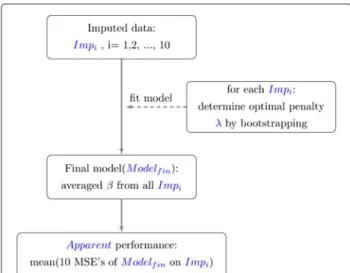
The discriminative performance of the best and tolerance models was quantified with the MSE. Enumerated below (shown schematically in Figure 1) are steps to acquire an averaged apparent MSE over the multiply imputed data.
Step 1: Construct a model in all 10 imputed data sets (original samples:Impi,i=1, 2, .., 10) as described in the previous section, and average the regression coefficients over all data sets to obtain one final model,Modelfin..
Step 2: UsingModelfin., determine the apparent performance onImpi. This results in 10 apparent performances (Apparenti).
Step 3: The finalApparent performance is the average over the 10Apparentiperformances.
To assess calibration, the predicted CRQ dyspnea out-come scores were plotted against the observed values, along with their averages by deciles of predicted values. The corresponding calibration line was described using a linear regression with the observed outcome regressed on the linear predictor (LP): CRQ dyspnea = αLP+βLP×
Figure 1A summary of the model construction steps and evaluation of performance via the lasso.
LP. The parameterβLP is termed calibration slope [24],
which can be seen as a uniform shrinkage factor [10,11]. A perfect calibration would yield a line withαLP =0 and βLP=1. For a clinically good calibration, the averages per
decile should be within a +/−0.5 limit of the minimal clinically important difference [25].
Validation
Bootstrap resampling for internal validation and estima-tion of the expected optimism was performed based on Harrell [6]. This was performed to validate our averaged final model from the previous section. First, we consid-ered validating the discrimination index, and below is a description of four approaches to handle the multiply imputed data sets in the validation procedure.
Approach 1: It is ensured that a bootstrap run selects the same subjects across the imputed data sets. Hence, bootstrap samples differ solely by the imputed values.
1. In a bootstrap draw select the same subjects over all
Impito getImp∗i.
2. Redo every model building step from step 1 in the original model construction (previous section). The performance ofModel∗fin.on eachImp∗i is evaluated and averaged to obtainApparent∗.
3. ApplyModelfin∗ .to the original samples,Impito determine the averaged test performance,Test∗
4. Calculate the optimism,Optimism∗as
Apparent∗−Test∗
5. Repeat 1 to 4 at least 100 times to obtain a stable estimate of the optimism.
6. The optimism-corrected performance,true
performance, is the difference of the Apparent (Step 3 in the Model performance section) and mean of the 100Optimism∗’s (estimated in 4).
A schematic summary of approach 1 is shown in Figure 2. If there are no missing data, the same data are used in all 10 “subsamples”.
Approach 2: Records selected in a bootstrap run can differ over the imputed data sets. Thus as opposed to approach 1, subjects were not forced to be the same over theImp∗i’s.
Approach 3: Select just one of the imputed data sets and perform the resampling procedure as in the case where there is no missing data.
Approach 4: This approach differs from the previous approaches in that it incorporates the MI procedure in the validation. Here, for step 1, a bootstrap sample was taken from the incomplete data set and then MI was performed 10 times. The procedure then proceeded as described in step 2 to step 6 of approach 1.
The amount of miscalibration was quantified via the calibration slope βLP. Correction was achieved by
re-estimating the intercept and multiplying each estimated effect with a shrinkage factor s [10,11] that was deter-mined as follows. In every bootstrap run, model construc-tion per imputed dataImp∗i was carried out as with the original sample Impi and values of the linear predictors
LP∗were calculated on the original samples. The intercept (αLP∗)and slope (βLP∗)of LP∗was estimated by
regress-ing the outcome in the original sample on the LP∗. This
Figure 2An algorithm to calculate optimism in the presence of multiply imputed data based on Harrell [6].Thetrue performance=Apparent (Step 3 in the Model performance section) - mean (BOptimism∗’s). B is the number of bootstrap samples and∗is used to denote bootstrap objects.
Musoroet al. BMC Medical Research Methodology2014,14:116 Page 5 of 13 http://www.biomedcentral.com/1471-2288/14/116
process was repeated 100 times ands was calculated as the mean of the 100 estimates ofβLP∗(β¯LP∗) [5,6,8]. The
re-calibrated model wasα¯LP∗+ ¯βLP∗(α+βTX). Usually,
¯
βLP∗ < 1, meaning that in the original model low
predic-tions of the outcome will be too low and high predicpredic-tions too high. In a case with over-shrinkage,β¯LP∗ > 1,
imply-ing that low predictions of the outcome will be too high and high predictions too low. Multiplying each coefficient byβ¯LP∗leads to shrinking (ifβ¯LP∗ <1) or unshrinking (if
¯
βLP∗ > 1), which usually improves both calibration and
MSE.
Software
All analyses were implemented using theRstatistical soft-ware, version 2.15.2 [26]. The mice package [21] was used to perform MI. Variable selection and model fitting was performed using the glmnet [27] and caret [28], packages. Additional routines were developed to perform the boot-strap resampling procedure in the presence of multiply imputed data (See Additional file 1).
Results
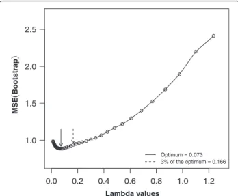
In Figure 3, a summary of the parameter tuning proce-dure, showing the bootstrap performance of all 40 penalty values (on one imputed data set) is given. This illustrates that an optimal λ value was identifiable. The optimal lambda varied between 0.063 and 0.082 over the imputed data sets for the best model, and between 0.064 and 0.166 for the tolerance model. In Table 1 we report averaged coefficients of the best and tolerance models, and the
0.0 0.2 0.4 0.6 0.8 1.0 1.2 1.0 1.5 2.0 2.5 Optimum = 0.073 3% of the optimum = 0.166 Lambda values MSE ( Bootstrap )
Figure 3Performance profile to determine the optimal lasso penalty tuning parameter (on one imputed data set) for a grid of 40 penalty values based on 100 bootstrap samples.The optimal penalty value corresponding to the best model is that which generated the smallest average MSE over the bootstrap samples. A tolerance model can be estimated as that with MSE within 3% of the optimum in the direction of the stronger penalties.
number of times each variable was retained across the imputed data sets. In total, 19 and 10 covariates were retained at least once across the imputed data sets for the best and tolerance model respectively. The estimated optimism, calculated according to the four approaches described above, along with the apparent and optimism-corrected MSE’s are presented in Table 2. The estimate of optimism was sensitive to the choice of handling imputed data in the bootstrap procedure. Estimates from approach 1, 3 and 4 suggested that there was substantial optimism in the apparent performance. Larger values of optimism were observed with approach 4. On the other hand, approach 2 suggested there was very little or no optimism.
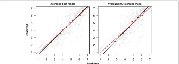
The calibration plots in Figure 4 show that there was over-shrinkage of the coefficients. This was more obvious with the tolerance model, which is to be expected since a stronger penalty was applied. TheβLP’s were greater than
1 (as shown by the solid black lines in Figure 4). Similar estimates ofβLP∗ were obtained over the four approaches (2). The calibration was improved after re-calibrating the coefficients. This is shown (for the case whereβLP∗ was estimated via approach 1) by the dashed red lines in Figure 4. The re-calibrated coefficients are also provided in Table 1.
Simulation study
Study setup
We simulated 20 covariatesXjfrom a multivariate normal
distribution with μj = 0 andσj = 1, for j = 1,2. . . , 20.
Most of the correlations were zero except for R1,5 = 0.72,R1,6 = −0.52,R2,8= 0.74,R4,12 = −0.82,R6,16 = − 0.34,R10,20 = −0.38,R11,19 = 0.37,R19,20 = 0.65.X1to
X10were categorized as binary covariates. Dichotomiza-tion ofX1,X2,X6andX7was at their respective 50th per-centile values. The categories forX3,X4,X8 andX9, and forX5andX10, was at their 30th and 20th percentile val-ues respectively. The regression coefficients were taken to beβ0(intercept)=1.14,β1toβ5=0,β6= −0.839,β7= 1.131,β8 = −1.540,β9 = 1.426,β10 = 0.854,β11 to β15 =0,β16 =0.457,β17 = −0.494,β18 = −0.738,β19= 1.589,β20=0.845. The outcome wasY =β0+XTβ+, where ∼ N(0,sd = 1.74). Nine out of the 20 covari-ates always contain missing values which were missing completely at random, with percentage of missing values based on draws from a binomial distribution;X2,X7,X12 andX17with a 20% chance of missing, andX3,X8,X13and
X18with a 50% chance of missing. There were no missing outcome data. For every simulated data set the following procedures were performed.
1. A lasso linear regression model with all covariates was fitted to the data in the setting without missing values (NM).
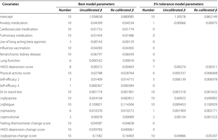
Table 1 Models with the best penalty value and the penalty within 3% of the optimum
Covariates Best model parameters 3% tolerance model parameters
Number Uncalibratedβ Re-calibratedβ Number Uncalibratedβ Re-calibratedβ
Intercept 10 1.038638 0.880085 10 1.30578 0.862149
Anxiety medication 10 -0.04399 -0.04534 1 -0.00066 -0.00075
Cardiovascular medication 10 -0.01752 -0.01774 0
Pulmonary medication 10 -0.01454 -0.01486 0
Use of long acting beta agonists 3 -0.00143 -0.00129 0
Influenza vaccination 10 -0.04283 -0.04365 0
Renal:chronic kidney disease 10 -0.06797 -0.06939 0
Lung function 6 0.000162 0.00018 0
HADS depression score 8 -0.00372 -0.00403 7 -0.00274 -0.00311
Physical activity score 10 0.02788 0.028764 6 0.005337 0.006068
Self-efficacy 2 3 0.01409 0.014715 3 0.006139 0.006978
Self-efficacy 3 1 0.000367 0.000384 0
Sit to stand test 10 0.001774 0.001901 10 0.001518 0.001632
crqdyspnea 10 0.654104 0.682812 10 0.60923 0.690902
crqfatigue 10 0.109821 0.114304 10 0.089453 0.100929
crqmastery 6 0.010376 0.010272 1 0.001909 0.002171
crqemotional 3 0.00078 0.00089 2 0.00134 0.001523
Feeling thermometer change score 10 -0.04587 -0.04658 0
HADS depression change score 10 0.039783 0.040061 0
crqdyspnea change score 10 -0.1582 -0.16403 10 -0.04866 -0.05207
The column “number” gives the number of times each variable was selected across the imputed data sets.
2. In the setting with missing data (WM), missing values were imputed 10 times using MICE and a lasso linear regression model was fitted to each imputed data set. Similar to the study data, the final model was an average of coefficients over the imputed data sets. Hence covariates that were estimated to be zero several times had small coefficients.
3. The expected optimism, referred to as
Optimisminternal, was estimated in the NM and WM settings respectively via bootstrap resampling as described by Harrell [6] and the four approaches described above. For both settings, the final models
were evaluated on the original sample and on a new independent data set (with no missing values) to obtainMSEapparentandMSEexternalrespectively. The observed optimism (Optimismexternal) was the difference betweenMSEapparentandMSEexternal. We would expectOptimisminternalandOptimismexternal
to be close if the resampling procedure gives unbiased estimates of optimism.
Simulation study results
We used sample sizes of n = 250 and 1000, and per-formed 1000 simulations. The results are summarized in
Table 2 Apparent and optimism-corrected MSE values based on the four approaches (“Appr 1”, “Appr 2”, “Appr 3” and “Appr 4”) of handling multiply imputed data sets, and the shrinkage factor (βLP¯ ∗)
MSE0=2.4183 Averaged best model 0.9047 Averaged 3% tolerance 0.9672
Apparent MSEX Appr 1 Appr 2 Appr 3 Appr 4 Appr 1 Appr 2 Appr 3 App 4
Optimism -0.1162 -0.0127 -0.0988 -0.1452 -0.0656 -0.0081 -0.0537 -0.0781
Optimism corrected MSEX 1.0209 0.9174 1.0035 1.0499 1.0328 0.9753 1.0209 1.0453
¯
Musoroet al. BMC Medical Research Methodology2014,14:116 Page 7 of 13 http://www.biomedcentral.com/1471-2288/14/116
Averaged best model
1 2 3 4 5 6 7 1 1 1 1 1 1 1 1 1 11 1 1 1 1 1 1 1 1 1 1 1 1 1 1 1 1 1 1 1 1 1 1 1 2 2 2 2 2 2 2 2 2 2 2 2222 2 2 2 2 2 2 2 2 2 2 2 2 2 22 2 2 2 3 3 3 3 3 3 3 3 3 3 3 3 3 3 3 3 33 3 3 3 3 3 3 3 3 3 3 3 3 3 3 3 4 4 4 4 4 4 44 4 4 4 4 4 4 4 4 4 4 4 4 4 44 44 4 4 4 4 4 4 4 4 5 5 5 5 5 5 5 5 5 5 5 5 55 5 5 5 5 5 5 5 5 5 5 5 5 5 5 55 5 5 5 6 6 6 66 6 6 6 6 6 6 6 6 6 6 6 6 6 6 6 6 6 6 6 6 6 6 6 6 6 6 6 6 7 7 7 7 7 7 7 7 7 7 7 7 7 7 7 7 7 7 7 7 7 7 7 7 7 7 7 7 7 7 77 7 8 8 8 8 8 8 8 8 8 8 8 8 8 8 8 8 8 8 8 8 8 8 8 8 8 8 8 8 8 88 8 8 9 9 9 9 9 9 9 9 9 9 9 9 9 9 99 9 9 9 9 9 9 99 9 9 9 9 9 9 9 9 9 10 10 10 10 10 10 10 10 101010 10 1010 10 10 10 10 10 10 10 10 10 101010 10 10 10 10 10 10 10 10
Averaged 3% tolerance model
1 2 3 4 5 6 7 1 1 1 1 1 1 1 1 1 1 1 1 1 1 1 1 1 1 1 1 1 1 1 1 1 1 1 1 1 1 1 1 1 1 2 2 2 2 22 2 2 2 22 22 2 2 2 2 2 2 2 2 2 2 2 2 2 2 2 2 2 2 2 2 3 3 3 3 3 3 3 3 3 3 3 3 3 3 3 33 33 3 3 3 3 3 3 3 3 3 3 3 3 3 3 4 4 4 4 4 4 4 4 4 4 4 4 44 4 4 4 4 4 4 4 4 4 4 4 4 4 4 4 4 4 4 4 5 5 5 5 5 5 5 5 5 5 5 5 5 5 5 5 5 5 5 5 5 5 55 5 5 5 5 5 5 5 5 5 6 6 6 6 6 6 6 6 6 6 6 6 6 6 6 6 6 6 6 6 6 6 6 6 66 6 6 6 6 6 6 6 7 7 7 7 7 7 7 7 7 7 7 7 7 7 7 7 7 7 7 7 7 7 7 7 7 77 7 7 7 7 7 7 8 8 8 8 8 8 8 8 8 8 8 8 8 8 8 8 88 8 8 8 8 8 8 8 8 8 8 8 8 8 8 8 9 99 9 9 9 9 9 9 9 9 99 99 9 9 9 9 99 9 9 9 9 9 9 9 99 9 9 9 10 10 10 10 10 10 10 10 10 10 1010 10 10 10 10 10 10 10 10 10 10 10 10 10 101010 10 10 10 10 10 10 Predicted Observed
Figure 4Plots of the observed against the predicted CRQ dyspnea (range from 1 (worst) to 7 (best)) at 12 months.The gray diagonal line represents perfect calibration. The black solid line and red dashed lines are the regression lines for uncalibrated and re-calibrated models. Black open triangular points and red filled square points are based on deciles of predicted CRQ dyspnea from the uncalibrated and re-calibrated models respectively. The dotted gray lines represent the+/−0.5 minimal clinically important difference. The raw data is represented by the gray points. The numbers indicate deciles to which they belong.
Figures 5, 6, 7, 8 and 9, and in Additional file 2: Table S1 which shows the means and corresponding 2.5th and 97.5th percentile values within parentheses.
Figures 5 and 6 give an impression of how frequent the relevant (βj = 0) and the irrelevant (βj = 0) covariates
were selected across the simulated data sets, withn=250. As earlier observed [29], the best model retained a large
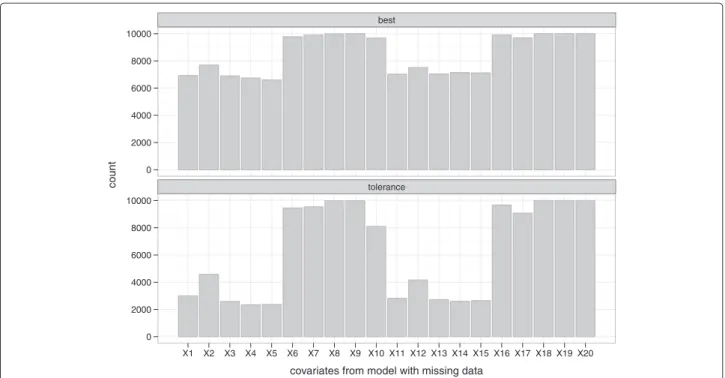
number of irrelevant covariates (X1toX5andX11toX15), with the selection frequency ranging from about 45% to 55% for the NM setting. This was higher for the WM set-ting (66% to 75%) because covariates were counted if they were included in at least one of the imputed date sets. A more desirable selection was achieved with the tolerance models; selection frequency of the irrelevant covariates in
best tolerance 0 200 400 600 800 1000 0 200 400 600 800 1000 X1 X2 X3 X4 X5 X6 X7 X8 X9 X10 X11 X12 X13 X14 X15 X16 X17 X18 X19 X20
covariates from model with no missing data
count
Figure 5Frequency of selection per covariate from the data without missing values (NM).“best” and “tolerance” correspond respectively to models with the optimal penalty (smallest MSE) and a penalty that has MSE within 3% of the optimum.
best tolerance 0 2000 4000 6000 8000 10000 0 2000 4000 6000 8000 10000 X1 X2 X3 X4 X5 X6 X7 X8 X9 X10 X11 X12 X13 X14 X15 X16 X17 X18 X19 X20
covariates from model with missing data
count
Figure 6Frequency of selection per covariate (retained at least once across the 10 imputed data sets) from the data with missing values (WM).“best” and “tolerance” correspond respectively to models with the optimal penalty (smallest MSE) and a penalty that has MSE within 3% of the optimum.
the range 11% to 20% and 25% to 47% for the NM and WM settings respectively. Similar findings were observed withn=1000, where much lower selection frequencies of the irrelevant covariates were observed for the tolerance model; ranging from 0% to 8% and 3% to 25% for the NM and WM settings respectively. Notice that the relevant covariates were selected much more frequently (selection frequency generally ranging from about 79% to 100%) than the irrelevant ones. In the NM setting, the lasso was able to find the correct model (that is with respect to selecting all the relevant predictors simultaneously) 97.1% and 76.8% of the time for the best and tolerance mod-els respectively. It was only one relevant variable off in about 2.9% and 22.2% of the time for the best and toler-ance models respectively. In the WM setting, considering the case where variables were retained in at least 50% of the imputed data sets, the correct model was selected about 97.6% and 75.7% of the time for the best and toler-ance models respectively. It was only one relevant variable off in about 2.3% and 21.5% of the time for the best and tolerance models respectively.
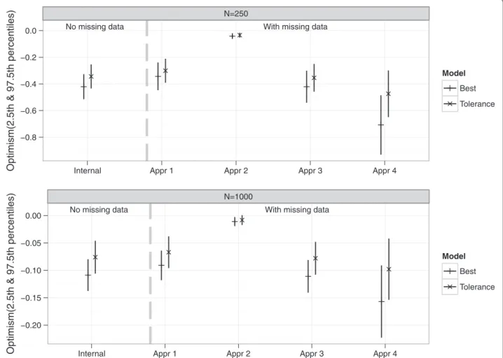
For both the NM and WM settings, the apparent MSE’s were optimistic. Estimates of optimism along with 2.5th and 97.5th percentiles are shown in Figure 7 for both NM and WM settings. In the NM setting and withn=250, the mean Optimisminternal −0.421 (best model) and−0.344
(tolerance model) were close to but significantly differ-ent from the meanOptimismexternal −0.410 and−0.324
for best and tolerance models respectively. With a larger sample size, n = 1000, the mean Optimisminternal and
Optimismexternalwere more similar and had smaller 2.5th
and 97.5th percentile values (see Additional file 2: Table S1). In the WM setting, the mean Optimisminternal
dif-fered significantly between the four approaches of han-dling imputed data in the validation procedure for both n = 250 and 1000. Histograms ofOptimisminternal from
these approaches are shown in Additional file 3: Figure S1 (n = 250). While the estimates from applying approach 1, 3 and 4 suggested that there was optimism in the apparent performance, findings from approach 2 on the other hand suggested little or no optimism. Similar to the real data example, larger values of optimism were obtained via approach 4. The meanOptimisminternalbased
on approach 3 (best = −0.421, tolerance = −0.354) was very similar to that obtained from the NM setting (best= −0.421, tolerance= −0.344), because both used just a single data set. Also, the meanOptimisminternalfrom
approach 1 (best = −0.343, tolerance = −0.301) and approach 3 were smaller than the meanOptimismexternal
(best = −0.668, tolerance = −0.467), while that from approach 4 (best = −0.708, tolerance = −0.474) was slightly larger. However with a larger samplen = 1000, apart from approach 2 which still suggested negligible optimism, the meanOptimisminternalandOptimismexternal
were much more similar for both the NM and WM set-tings (see Additional file 2: Table S1). Figure 8 summarizes
Musoroet al. BMC Medical Research Methodology2014,14:116 Page 9 of 13 http://www.biomedcentral.com/1471-2288/14/116
No missing data With missing data N=250 −0.8 −0.6 −0.4 −0.2 0.0
Internal Appr 1 Appr 2 Appr 3 Appr 4
Optimism(2.5th & 97.5th percentiles)
Model
Best Tolerance
No missing data With missing data N=1000 −0.20 −0.15 −0.10 −0.05 0.00
Internal Appr 1 Appr 2 Appr 3 Appr 4
Optimism(2.5th & 97.5th percentiles)
Model
Best Tolerance
Figure 7Estimates of optimism from the simulation study.Optimism “Internal” was the difference between the bootstrap performance (on bootstrap data) and the test performance (on original data). Optimism “Appr 1”, “Appr 2”, “Appr 3” and “Appr 4” were based on the four approaches of handling missing data.
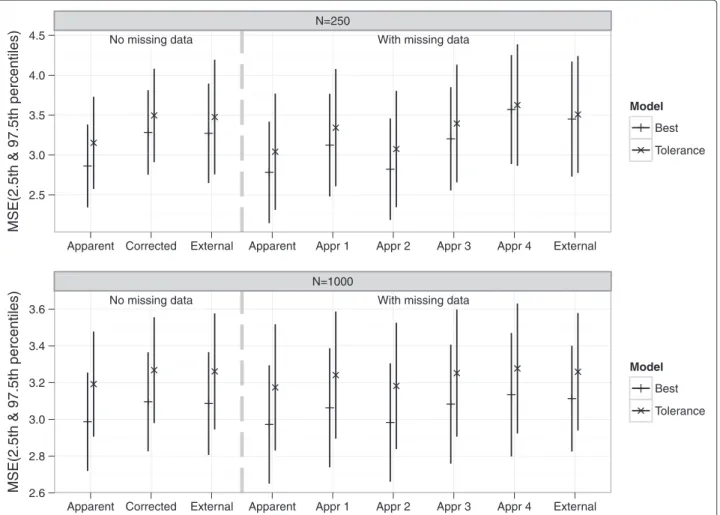
the estimated MSE values. Compared to the NM setting, theMSEexternal was larger for the WM setting (probably
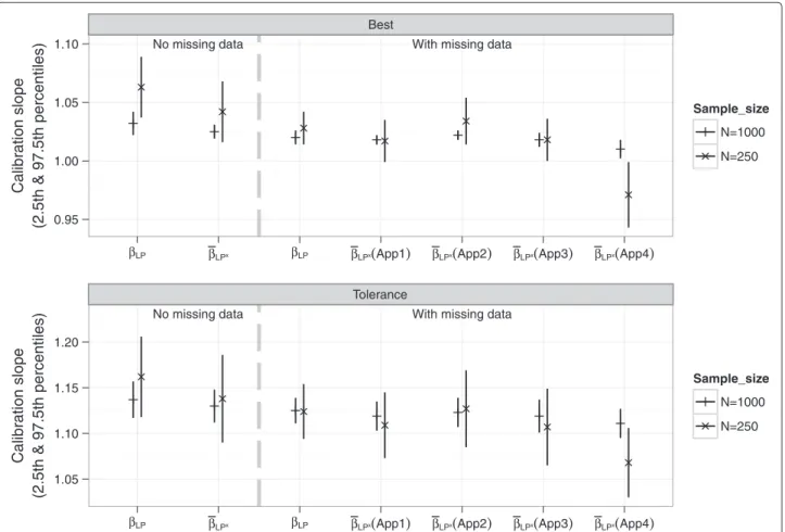
because more irrelevant covariates were retained). There was suboptimal calibration due to over-shrinkage, apparent from the meanβLP’s which were>1
in both the NM and WM settings with bothn=250 and 1000. As expected there was more shrinkage with the tol-erance (tol) model since it applied a stronger penalty. The means ofβ¯LP∗ also differed between the four approaches
of handling imputed data in the resampling procedure. Estimates from all 4 approaches were more similar to each other for the larger sample sizen = 1000 (see Figure 9 and Additional file 2: Table S1).
Discussion
We constructed models to predict CRQ dyspnea 6 months ahead for a cohort of COPD patients by using the lasso technique. This approach combines shrinkage and vari-able selection, and is promising when prediction and parsimony are goals of predictive modelling. It can also be
applied to generalized linear models such as the logistic or Cox model [1,2]. Multiple imputation (MI) was imple-mented to cater for incomplete data, and the optimal lasso penalty for each imputed data set was determined via bootstrapping.
Nineteen predictors were retained by the best model (with the optimal penalty), which may be an unreasonable large number of predictors to use in practice. A stronger penalty can be applied to pick a smaller subset of covari-ates without sacrificing too much performance. Here for instance we chose a stronger penalty that had the MSE within 3% of the optimum, resulting to a reduced sub-set of 10 covariates. Another approach would be to apply a “majority method” that selects only variables that were retained in all imputed data sets. However, though par-simony is desired for practice, it is often at the expense of a lower predictive performance. On the other hand the lasso prevents overfitting. But the large variability in the set of selected predictors as demonstrated in our simulation study and earlier by Van Houwelingen [29]
No missing data With missing data N=250 2.5 3.0 3.5 4.0 4.5
Apparent Corrected External Apparent Appr 1 Appr 2 Appr 3 Appr 4 External
MSE(2.5th & 97.5th percentiles)
Model
Best Tolerance
No missing data With missing data N=1000 2.6 2.8 3.0 3.2 3.4 3.6
Apparent Corrected External Apparent Appr 1 Appr 2 Appr 3 Appr 4 External
MSE(2.5th & 97.5th percentiles)
Model
Best Tolerance
Figure 8Means of estimated MSE values from the simulation study.MSE “Apparent” was the performance on the original data. MSE
“Corrected”=MSEapparent−OptimisminternalMSE “External” was the performance on an independent new data with no missing values MSE “Appr 1”,
“Appr 2”, “Appr 3” and “Appr 4” were based on subtracting the value of optimism estimated via the four approaches of handling missing data from MSEapparent(with missing data).
is unappealing. It was observed in our simulation study that the final best models often retained all the rele-vant covariates but were also commonly contaminated with irrelevant covariates, especially in the WM set-tings. There was less contamination with the tolerance models.
The calibration plots showed that there was over-shrinkage of coefficients. Also, applying the lasso resulted in optimistic estimates of model performance. This implies that the lasso penalty chosen via bootstrapping was optimal only for the data at hand. The same was observed in the simulation study for both the setting with (NM) and without (WM) missing data. Thus, as most model building procedures, the model constructed via the lasso still requires validation. Moreover, it has the ten-dency of retaining redundant covariates. This was more frequent for WM settings since different variables could be selected for different imputed data sets. Some ways to handle variable selection over multiply imputed data
sets have been addressed in the literature [30-33]. The multiple imputation lasso (MI-LASSO), which applies a group lasso penalty, has been proposed to select the same variables across multiply-imputed data sets [31]. A com-parable level of parsimony and model performance was observed between the MI-LASSO model and our toler-ance model with both the real data and the simulated data sets. In the simulation study, we observed that the frequency of selection of the relevant (X6 to X10 and
X16 to X20) and irrelevant (X1 to X5 and X11 to X15) covariates using the MI-LASSO technique was very sim-ilar to that obtained using our tolerance model. The selection frequency of the irrelevant covariates was in the range of 25% to 47% for our tolerance model and 25% to 65% for the MI-LASSO. The mean MSEcorrected
(MSEexternalwithin parentheses) over the 1000 simulated
data set (n= 250, approach= 4) was 3.559 (3.440) and 3.626 (3.508) for the MI-LASSO and our tolerance model respectively.
Musoroet al. BMC Medical Research Methodology2014,14:116 Page 11 of 13 http://www.biomedcentral.com/1471-2288/14/116
No missing data With missing data Best
0.95 1.00 1.05 1.10
βLP βLPx βLP βLPx(App1) βLPx(App2) βLPx(App3) βLPx(App4)
Calibration slope
(2.5th & 97.5th percentiles)
Sample_size
N=1000 N=250
No missing data With missing data Tolerance
1.05 1.10 1.15 1.20
βLP βLPx βLP βLPx(App1) βLPx(App2) βLPx(App3) βLPx(App4)
Calibration slop e (2.5th & 97.5th percentiles) Sample_size N=1000 N=250
Figure 9Means of estimated of calibration slope parameters from the simulation study.βLPwas the slope of the the linear predictor (LP)
estimated from regressing the observed outcome on LP from the original data.β¯LP∗(shrinkage factor) was the slope ofLP∗estimated by regressing
the outcome in the original sample on theLP∗from the bootstrap sample.
The estimate of optimism was sensitive to the choice of handling the imputed data sets in the bootstrap resam-pling procedure. This was observed with both the study and simulated data sets. The results based on approach 1, 3 and 4 suggested that the lasso models were optimistic.
Approach 1, 2 and 3 were performed by resampling data sets that had been completed via MI, and an important question was how to sample subjects over the imputed data sets. Approach 1 ensured that for a bootstrap draw, the samples from each imputed data set differed only by the imputed values as in the original data sets. In approach 2, bootstrap samples over the imputed data could differ by the imputed values as well as the selected subjects. This led to an underestimation of optimism (discussed in the next paragraph). Approach 3 performed the vali-dation procedure using only one imputed data set. This was easier to perform as it mimicked the procedure where there was no missing data, and required less bookkeeping. Approach 4 on the other hand resampled the incomplete data set and then applied MI, thus incorporating the MI procedure in the validation. In the simulation study, the meanOptimisminternal from approach 1 was significantly
smaller than that from approach 3, and both were biased downward with respect to the meanOptimismexternal. In
the case of approach 4, the mean Optimisminternal was
more similar to Optimismexternal, though slightly biased
upward. The same was observed with the NM setting. A more upward bias was observed when approach 4 was performed such that only one imputation was derived from a bootstrap sample taken from the original data with missing values. So we advise to use multiple imputations. The biases from approach 1, 3 and 4 were smaller for n=1000, where a smaller number of irrelevant covariates were retained compared to when n=250, and were much smaller with the tolerance models.
Contrary to approach 1, 3 and 4, approach 2 clearly underestimated optimism sinceMSEcorrectedfor bothn=
250 and 1000 were lower than MSEexternal, and even
lower than the theoretical MSE (1.742 = 3.028). The explanation is that a bootstrap draw across the imputed data sets differed by both the imputed values as well as the selected subjects, introducing more heterogene-ity between the bootstrap imputed data sets than there should be. Consequently a more robust final model (that
averaged coefficients from all 10 data sets) was achieved. The performance of this model was similar in both the bootstrap and the original samples, leading to a negligi-ble estimate of optimism as observed with both the real data and in the simulation study. Approach 2 was repeated using 10 copies of the same data with no missing val-ues, mimicking a set-up with 10 multiply imputed data. This still gave very small values ofOptimisminternal, which
wrongly suggested negligible optimism.
Conclusions
We advise that prognostic models constructed via the lasso technique should also be evaluated for optimism. When data are missing and resampling techniques are used to estimate optimism, it does matter how multi-ply imputed data sets are handled. Improper handling of the multiply imputed data sets might results in substan-tially large underestimation of optimism as is the case with approach 2. We recommend approach 4 since it fully replays every step that was performed with the original data with missing values, and yields estimates of optimism that are close to theOptimismexternal.
Additional files
Additional file 1: R function to perform resampling with caret package in the presence of multiply imputed data.The “validate.train” function below estimates optimism in predictive value via the bootstrap resampling procedures described in approach 1 and 4 in the manuscript. In approach 1 the completed data sets (via MI) are resampled. The same subjects are selected across the imputed data sets so that the bootstrap imputed data sets always differ only by their imputed values. In approach 4, the incomplete data set is resampled and then MI is performed using the mice package. The function can be used to estimate optimism in the predictive value of a linear regression model constructed withincaret using thetrain()function, with method=“glmnet”. In order to be consistent with the output from caret, we assumed that the response variable is always in the last column of every data set.
Additional file 2: Table S1.Simulation study results. The table presents means of all estimates along with their corresponding 2.5th and 97.5th percentile values within parentheses. These are based on 1000 simulated data sets for both n=250 and 1000.
Additional file 3: Figure S1.Distribution of the estimated expected optimism values from the simulation study. These are based on 1000 simulated data sets (n=250) for both the setting without (NM) and with (WM) missing data.
Competing interests
The authors declare that they have no competing interests.
Authors’ contributions
Authors JM, AZ and RG devised the statistical methods. Authors MP and GtR were responsible for the design and data collection of the study. Author JM performed the statistical analysis and wrote the paper. All authors read and corrected the draft versions of the manuscript, and approved the final manuscript.
Acknowledgements
We would like to thank Lara Siebeling for participating in the planning and design of the study, and preparing the data for analysis.
Author details
1Department of Clinical Epidemiology, Biostatistics and Bioinformatics,
Academic Medical Center, University of Amsterdam, Meibergdreef 9, 1105 Amsterdam, the Netherlands.2Department of General Practice, Academic Medical Center, University of Amsterdam, Meibergdreef 9, 1105 Amsterdam, the Netherlands.3Institute for Social and Preventive Medicine, University of Zurich, Hirschengraben 84, CH-8001 Zurich, Switzerland.
Received: 13 March 2014 Accepted: 10 October 2014 Published: 16 October 2014
References
1. Tibshirani R:Regression shrinkage and selection via lasso.J Roy Stat
Soc B1996,58:267–288.
2. Tibshirani R:The lasso method for variable selection in the Cox model.Stat Med1997,16:385–395.
3. Steyerberg EW:Clinical Prediction Models: A Practical Approach to
Development, Validation, and Updating. New York: Springer; 2010.
4. Justice AC, Covinsky KE, Berlin JA:Assessing the generalizability of prognostic information.Ann Intern Med1999,130:515–524. 5. Steyerberg EW, Harrell FE, Borsboom GJ, Eijkemans MJ, Vergouwe Y,
Habbema JD:Internal validation of predictive models: efficiency of some procedures for logistic regression analysis.J Clin Epidemiol
2001,8:774–781.
6. Harrell FE, Lee KL, Mark DB:Multivariate prognostic models: issues in developing models, evaluating assumptions and accuracy, and measuring and reducing errors.Stat Med1996,15:361–387.
7. Breiman L:The little bootstrap and other methods for dimensionality selection in regression: X-fixed prediction error.J Am Stat Assoc1992,
87:738–754.
8. Efron B, Tibshirani RJ:An Introduction to the Bootstrap. New York: Chapman & Hall; 1986.
9. Harrell FE:Regression Modeling Strategies: with Applications to Linear
Models, Logistic Regression, and Survival Analysis. New York: Springer; 2001.
10. Van Houwelingen JC, Le Cessie S:Predictive value of statistical models.Stat Med1990,9:1303–1325.
11. Copas JB:Regression, prediction and shrinkage.J Roy Stat Soc B1983,
45:311–354.
12. Heymans MW, van Buuren S, Knol DL, van Mechelen W, de Vet HCW:
Variable selection under multiple imputation using the bootstrap in a prognostic study.BMC Med Res Methodol2007,7:33.
13. Rubin DB:Multiple Imputation for Nonresponse in Surveys. New York: John Wiley & Sons; 1987.
14. White IR, Royston P, Wood AM:Multiple imputation using chained equations: issues and guidance for practice.Stat Med2011,
30:377–399.
15. Vergouwe Y, Royston P, Moons KG, Altman DG:Development and validation of a prediction model with missing predictor data: a practical approach.J Clin Epidemiol2010,63:205–214.
16. Vergouw D, Heymans MW, Peat GM, Kuijpers T, Croft PR, de Vet HCW, van der Horst HE, van der Windt DAWM:The search for stable prognostic models in multiple imputed data sets.BMC Med Res Methodol2010,
10:81.
17. Siebeling L, Puhan MA, Muggensturm P, Zoller M, ter Riet G:
Characteristics of Dutch and Swiss primary care COPD patients -baseline data of the ICE COLD ERIC study.Clin Epidemiol2011,
3:273–283.
18. Siebeling L, ter Riet G, van der Wal WM, Geskus RB, Zoller M, Muggensturm P, Joleska I, Puhan MA:Ice cold eric–international collaborative effort on chronic obstructive lung disease:
exacerbation risk index cohorts–study protocol for an international copd cohort study.BMC Pulm Med2009,9:16.
19. Puhan MA, Behnke M, Frey M, Grueter T, Brandli O, Lichtenschop A, Guyatt GH, Schunemann HJ:Self-administration and interviewer-administration of the German chronic respiratory questionnaire: instrument development and assessment of validity and reliability in two randomised studies.Health Qual Life Outcomes2004,2:1. 20. Puhan MA, Behnke M, Laschke M, Lichtenschopf A, Brändli O, Guyatt GH,
Schünemann HJ:Self-administration and standardisation of the chronic respiratory questionnaire: a randomised trial in three German-speaking countries.Respir Med2004,98:342–350.
Musoroet al. BMC Medical Research Methodology2014,14:116 Page 13 of 13 http://www.biomedcentral.com/1471-2288/14/116
21. van Buuren S, Karin G:Mice: multivariate imputation by chained equations in R.J Stat Software2011,45:1–67.
22. Moons KGM, Donders RART, Stijnen T, Harrell FE:Using the outcome for imputation of missing predictor values was preferred.J Clin Epidemiol
2006,59:1092–1101.
23. vonHippel PT:Regression with missing Ys: an improved strategy for analyzing multiply imputed data.Socio Meth2007,37:83–117. 24. Cox DR:Two further applications of a model for binary regression.
Biometrika1958,45:562–565.
25. Schunemann HJ, Puhan M, Goldstein R, Jaeschke R, Guyatt GH:
Measurement properties and interpretability of the chronic respiratory disease questionnaire (crq).COPD2005,2:81–89. 26. R Core Team:R: A Language and Environment for Statistical Computing.
Vienna: R foundation for statistical computing; 2012. R foundation for statistical computing. ISBN 3-900051-07-0. [http://www.R-project.org/] 27. Friedman J, Hastie T, Tibshirani R:Regularization paths for generalized
linear models via coordinate descent.J Stat Software2010,33:1–22. 28. Kuhn M, Contributions from Wing J, Weston S, Williams A, Keefer C,
Engelhardt A:Caret: Classification and Regression Training.2012. R package version 5.15-023. [http://CRAN.R-project.org/package=caret] 29. Van Houwelingen JC, Sauerbrei W:Cross-validation, shrinkage and
variable selection in linear regression revisited.Open J Stat2013,3:79. 30. Wan Y, Datta S, Conklin DJ, Kong M:Variable selection models based
on multiple imputation with an application for predicting median effective dose and maximum effect.J Stat Comput Simulat2014:1–15 doi:10.1080/00949655.2014.907801.
31. Chen Q, Wang S:Variable selection for multiply-imputed data with application to dioxin exposure study.Stat Med2013,32:3646–3659. 32. Wood AM, White IR, Royston P:How should variable selection be
performed with multiply imputed data?Stat Med2008,27:3227–3246. 33. Yang X, Belin TR, Boscardin W:Imputation and variable selection in
linear regression models with missing covariates.Biometrics2005,
61:498–506.
doi:10.1186/1471-2288-14-116
Cite this article as:Musoroet al.:Validation of prediction models based on lasso regression with multiply imputed data.BMC Medical Research Methodology201414:116.
Submit your next manuscript to BioMed Central and take full advantage of:
• Convenient online submission • Thorough peer review
• No space constraints or color figure charges • Immediate publication on acceptance
• Inclusion in PubMed, CAS, Scopus and Google Scholar • Research which is freely available for redistribution
Submit your manuscript at www.biomedcentral.com/submit
![Figure 2 An algorithm to calculate optimism in the presence of multiply imputed data based on Harrell [6]](https://thumb-us.123doks.com/thumbv2/123dok_us/9329792.2811471/6.892.89.808.729.1047/figure-algorithm-calculate-optimism-presence-multiply-imputed-harrell.webp)