Working Paper 07-84
Statistics and Econometrics Series 18 December 2007
Departamento de Estadística Universidad Carlos III de Madrid
Calle Madrid, 126 28903 Getafe (Spain) Fax (34) 91 624-98-49
Forecasting from one day to one week ahead for the
Spanish system operator
José Ramón Cancelo1, Antoni Espasa2 and Rosmarie Grafe3
Abstract
This paper discusses the building process and models used by Red Eléctrica de España (REE), the Spanish system operator, in short-term electricity load forecasting. REE's forecasting system consists of one daily model and 24 hourly models with a common structure. There are two types of forecasts of special interest to REE, several days ahead predictions for daily data and one day ahead hourly forecasts. Accordingly, forecast accuracy is assessed in terms of their errors. For doing so we analyze historical, real time forecasting errors for daily and hourly data for the year 2006, and report forecasting performance by day of the week, time of the year and type of day. Other aspects of the prediction problem, like the influence of the errors in predicting temperature on forecasting the load several days ahead, or the need for an adequate treatment of special days, are also investigated.
Keywords: energy forecasting, hourly and daily models, time series, forecasting practice
1
José Ramón Cancelo, Universidades da Coruña, Dpto. Economía Aplicada II, Facultad de Ciencias Económicas, Campus de Elvira. 15008 A Coruña, España, phone: (34) 981167000-2512, fax: (34) 981167070, email: [email protected]
2 Antoni Espasa, Universidad Carlos III de Madrid, Statistics Department, C/Madrid, 126, 28903 Getafe (Madrid), Spain, phone: (34) 916249803, email: [email protected]
3 Rosmarie Grafe, Red Eléctrica de España, Pº del Conde de los Gaitanes, 177, 28109 Alcobendas (Madrid), Spain, phone: (34) 916502012-2314, fax: (34) 916504542, email: [email protected]
ACKNOWLEDGMENTS
We gratefully acknowledge the invaluable help and support we have always received from REE in the development of this project, with a special mention for Agustín Maure, Technical Secretary, Ventura Rodríguez, head of the Department of Statistics and Information, and Juan Moreno, Operation Director. We are also grateful to an anonymous referee and the guest editor James Taylor for their very useful comments. The second author gratefully acknowledges financial support from the Spanish Ministry of Education with the SEJ2006-03919/ECON grant.
1. INTRODUCTION
Short-term load forecasting has long been a major issue of interest for the electricity industry. Traditionally, hourly forecasts with a lead time of one hour to seven days are required for the scheduling and control of power systems. From the perspective of the system operators and regulatory agencies, they are a primary input for the safe and reliable operation of the system. For producers, they are a basic tool for determining the optimal utilization of generators and power stations, as some facilities are more efficient than others. Since the rise of free electricity markets that followed the deregulation of the power industry in the nineties, more agents became interested in load forecasting. Nowadays there is a huge variety of market participants, bidding strategies are more and more complex, and a number of financial derivatives have been developed. Commercial success depends on the ability to submit competitive bids, and even marginal improvements in forecasting the load can lead to substantial increases in trading profits. Nevertheless, the fact that a widespread demand for load forecasts exists does not entail that all agents are concerned with the same issues, as each organization seeks particular aims, and making explicit the actual needs of information of the organization is a prerequisite to set up fully adequate forecasting devices.
This paper describes the forecasting experience at Red Eléctrica de España (REE), based on different modelling projects developed by the authors since 1988. Load forecasting is a central activity within REE, and the search for a forecasting system able to encompass all short-term load forecasting tasks has long been a priority. Forecasting success is important and a necessary condition for validating any model. But the models are also internal tools that have to adapt to the operational features of REE and play a leading role in the acquisition, sharing, and use of knowledge within the organization
(Schultz 1992, Nevis et al 1995, Cancelo and Espasa 2001). As such, they are at the end of a sequence that begins by identifying the needs of REE, the kind of information forecasts are asked to provide, critical origins and lead times, and how to implement forecasting tools to promote organizational learning, i.e., the capacity to improve performance based on experience. In this sense, models are not aimed to produce tentative estimates that should be further elaborated by the control operator in duty to derive the final predictions of the load. On the contrary, the forecasting procedures seek to capture the knowledge of the qualified staff of the organization, and hence their implication in developing and monitoring the models is a major necessary condition for their success.
The paper is organized as follows. Section 2 summarizes the stylized features of the load data for mainland Spain to give a general view of the forecasting problem. Section 3 reviews the foundations of the models that integrate REE's forecasting system. After a general introduction, we sketch their main characteristics, report some estimated effects, and compare REE's approach to other procedures that have been suggested in the literature. Section 4 evaluates forecasting performance. Section 5 concludes.
2. LOAD DATA IN MAINLAND SPAIN: STYLIZED FACTS
The main features of load series have been extensively reported in the literature: trend, superimposed levels of seasonality, short-term dynamics, special days, nonlinear effects of meteorological variables, possible nonlinear time dependence, etc., see for instance Espasa et al (1996) in a general context of daily series of economic activity. Such features are not independent, observed series displaying a great variety of profiles according to the relative importance of each underlying component and the way they interact.
Centring on the particular traits of mainland Spain, it covers an area of almost 500,000 square kilometres with more than 42 million people. Average daily electricity consumption in 2005 was 677 GWh. The winter peak was 851 GWh and the summer peak 786 GWh. Figures 1 to 5 highlight some of the major characteristics of the load series. Figure 1 plots the monthly series to obtain a clearer picture of the trend. It shows the original series and the trend computed with a Hodrick-Prescott filter with λ=14,400, the default value for monthly data.
INSERT FIGURE 1 HERE
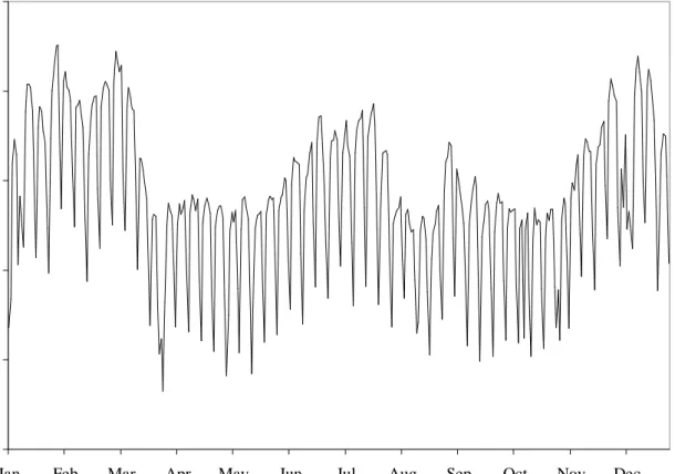
Figure 2 depicts daily consumption during 2005. Several intra-annual components can be observed: the weekly seasonal cycle, the weather-sensitive part of the load related to temperature effects in winter and in summer, and the influence of the vacation period in August. Annual seasonality is closely related to meteorological variables and vacation periods. Weekly and annual seasonalities are not independent, as, for instance, weekly seasonality is less pronounced in August than in any other month.
INSERT FIGURE 2 HERE
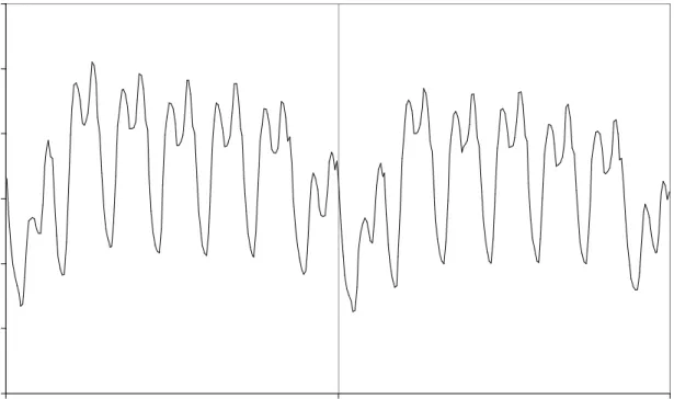
Figure 3 focus on intraday patterns. A fortnight of hourly data is displayed in each panel, and the figure shows that daily periodic behaviour varies both with the day of the week and the time of the year.
INSERT FIGURE 3 HERE
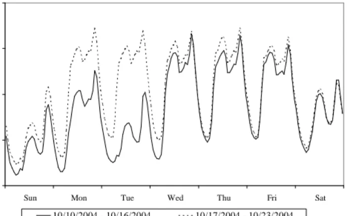
Figure 4 reports the alterations in the load when a special day occurs. The four panels refer to the same public holiday, October 12, on two consecutive years; panels A and B are for the holiday falling on a Tuesday, and panels C and D for the holiday on a Wednesday. It can be seen that the effects of special days are not independent of the weekly seasonal factor, and they can also be shown to be related to the annual seasonality.
INSERT FIGURE 4 HERE
Forecasting special days is a key issue for system operators, especially in Spain due to the idiosyncratic characteristics of the Spanish calendar. Most public holidays are observed on the same calendar date each year, but whenever a holiday falls on Sunday regional authorities can remove it to any other date of the year. The maximum number of public holidays is 14: 4 nationwide holidays, 2 local holidays, and the regional governments set the rest. Each region's authorities decide the number of holidays as long as the total does not exceed 14, and the dates that replace national holidays falling on Sunday. Regional governments tend to observe traditional Spanish holidays and in practice the resulting calendar is rather homogeneous across regions, yet there are some holidays that are region-specific and the total number of holidays within a given year may not be the same in all regions, or can vary in the same region from one year to the next. In 2006 there were 29 national or regional holidays, with very different effects on mainland Spain consumption of electricity. Local holidays in some big cities, notably Madrid (3.1 million people) and Barcelona (1.6 million), must be taken into account too, as they have perceptible effects on the total load. Special days also comprise long weekends arising from holidays that fall on Tuesday or Thursday / Friday and three vacation periods (August, Easter and Christmas). To sum up, special days and weekends represent from 33% to 45% of the days within a given year, depending on how strict the definition of a special day one considers.
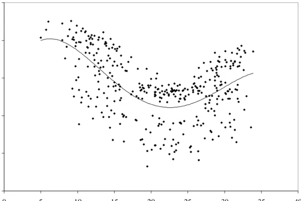
Figure 5 focuses on the relation between consumption and maximum temperature for daily data during 2005; a fourth-order polynomial was fitted to give a tentative indication of its shape. The relation is U-shaped and (could be) asymmetric, as the left branch is more pronounced than the right wing. There is also some evidence of an exhaustion effect, especially for low temperatures.
INSERT FIGURE 5 HERE
3. REVIEW OF THE MODELS 3.1 The basic strategy
The forecasting system currently implemented in REE consists of one daily model to forecast the daily load up to ten days ahead, and 24 hourly models to compute hourly predictions for horizons up to three days. The daily model is aimed to produce forecasts for network outage planning, while the hourly models are used to derive forecasts for next-day hourly dispatch.
This combination of 1+24 models has proven to be the best approach according to REE's needs. Daily forecasts up to ten days ahead for outage planning could be obtained from the hourly models, by computing 24 hourly forecasts for each day and adding them up to get the daily total. This procedure, however, renders forecasts with too much uncertainty for lead times up to ten days ahead, while a direct prediction of the daily aggregate provides a more adequate anchor. In a second step, and in order to derive the hourly forecasts that are required to complete the final outage plan, hourly models are used to compute the shape of the load curve for each day, and the daily forecasts are interpolated according to the predicted load curves.
For horizons up to three days, in contrast, direct hourly forecasts are more accurate than interpolated daily figures. Although there is some controversy as to whether it is better to treat each hour as a different series (Ramanathan et al 1997, Cottet and Smith 2003) or to build a single model to derive the load profile (Smith 2000, Taylor et al 2006), most authors prefer the first approach. REE's experience since 1988 supports that view, as separate models can be easily specified in a very flexible
way to capture short-term dynamics and the effects of special days and meteorological variables at different times of day.
All the models share a common basic structure, related to the traditional decomposition of the observed load into four components: normal load, the weather sensitive part, special events and a random component (Schneider et al 1985, Hyde and Hodnett 1997, Chen et al 2001). They are given a common type of response functions with parameters that are allowed to vary across series. The full search for specification was carried out in building the daily model, as the stylized features of the load in the aggregated daily data are also present in the daily series corresponding to each hour. Let Ct denote electricity consumption at day t and assume that the model is additive in logarithms: ) 1 ( u CWEA CSD s p C ln t = t + t + t + t + t
pt+st is the normal load, where pt denotes the trend and st (part of) the seasonal; CSDt is the contribution of special days; CWEAt is the contribution of meteorological variables; ut is a stationary disturbance that may display some short-term, transitory dynamics. In practice it is not easy to separate annual seasonality from the effect of weather variables, so in the daily model st consists basically of weekly seasonals. In fact, most annual seasonality can be explained by weather variables and by dummy variables that take account of vacation periods.
In the rest of Section 3.1 we give a rough, general sketch of the way each component is modelled. Next, some alternative approaches are reviewed in Section 3.2, where we also explain why we opted for the specification that follows, and report some estimated effects to give some insight on the dependence of the electricity consumption on special days and temperature.
) 2 ( u s p CWEA CSD C ln BC ln t = t − t − t = t + t + t
It represents the load that would be observed if there were no further effects from special days or weather variables. Since these additional effects are the major disturbances that alter the observed load, BCt is rather smooth and can be assumed to follow, at least as an approximation, an ARIMA model:
) 3 ( a ) L ( BC ln ) L ( ) L ( ∆ t = θ t φ
where φ(L) and θ(L) are polynomials in the lag operator L with all their roots outside the unit circle, ∆(L) is a polynomial with unit roots and at is a white noise process. Figures 1 and 2 suggest that a reasonable specification for ∆(L) is ∆∆7=(1-L)(1-L7), as the series display a local linear trend and a strong weekly seasonal pattern which is nondeterministic and is not explained by exogenous variables. If the stationary AR and MA polynomials are specified in a multiplicative form with three factors, a regular one on the operator L, a weekly seasonal on L7 and an annual seasonal on L365, the final expression of the ARIMA model for the basic consumption follows:
) 4 ( a ) L ( ) L ( ) L ( BC ln ) L ( ) L ( ) L ( t 365 365 7 7 t 7 365 365 7 7 Φ ∆∆ = θ Θ Θ Φ φ
Once the basic load is defined, special days and weather effects are introduced by extending the model to include dummy and weather variables. Their effects on the load are dynamic and may depend on the day of the week and the time of the year. In the case of the dummies for special days, adding leads and lags is a parsimonious way of representing the effect on adjacent days, while the dynamic weather effects reflect that individuals adjust to changing weather conditions with some delay. The nonlinear relation between consumption and temperature is modelled by computing several degree-days transformations of the observed temperatures, which will be explained in detail in Section 3.2. The model includes other meteorological variables like cloudiness
load, but are not considered because no reliable forecasts are produced and therefore they provide no relevant information for load forecasting.
The joint contribution of special days and weather variables can be expressed as:
) 5 ( WEA ) L ( SD ) L ( CWEA CSD n 1 j t , j i m 1 i t , i i t t
∑
∑
= = β + α = +where SD1,t, SD2,t, ..., SDm,t are m dummy variables that define the different classes of special days, WEA1,t, WEA2,t, ..., WEAn,t represent n transformations of the observed meteorological variables, and αi(L), βj(L), i=1,..,m, j=1,...,n, are lag polynomials.
To derive the final expression for the observed load, from (4) and (5) it follows that ) 6 ( a ) L ( ) L ( ) L ( ) L ( ) L ( ) L ( WEA ) L ( SD ) L ( C ln t 7 365 365 7 7 365 365 7 7 n 1 j t , j i m 1 i t , i i t ∆ ∆ Φ Φ φ Θ Θ θ + β + α =
∑
∑
= =The final specification of model (6) was derived by starting from an ARIMA model with dummy variables to capture the influence of special days; at this first stage, no effects of weather variables were considered. Next, the model was extended to include a basic response to temperature, and in subsequent versions this response was allowed to be more and more complex to capture the variety of effects that are reviewed in Section 3.2. Finally, other meteorological variables were tested to assess whether they actually improve the forecasting performance of the model, and the final response to weather conditions was derived. Search for specification centred on the daily series; once a final, satisfactory daily model was achieved, its parameters were reestimated for each hourly series to get the final hourly models. As a general result, it was found that the hourly models are not as complex as the daily model, because many meteorological effects are not significant for specific hours within the day.
3.2 Description of the models Basic load
Several procedures have been proposed to take account of the trend. Some studies get rid of it by taking short samples where the mean level of the load can be assumed to be constant (Smith, 2000). Others consider a variety of deterministic functions of time: linear (Pardo et al 2002), linear and reciprocal (Ramanathan et al,
1997), quadratic (Cottet and Smith, 2003), etc. Deterministic seasonal components include dummy variables (Ramanathan et al 1997, Soares and Souza 2006) and
time-varying periodic splines (Harvey and Koopman, 1993). Methods for explaining short-term time dependence comprise linear autoregressions (Pardo et al 2002, Cottet and
Smith 2003), fractionally integrated processes (Soares and Souza, 2006), artificial neural networks (Lamedica et al 1996, Darbellay and Slama 2000, Chen et al 2001,
Hippert et al 2005), double seasonal Holt-Winters exponential smoothing adjusted for
error correlation (Taylor, 2003), etc.
Our proposal for the basic load is simple and yet highly effective. The two real, positive unit roots embedded in the ∆∆7 operator generate a local linear trend that is flexible enough to approximate a wide variety of situations, and a large sample can be used for estimating the model without needing to concern about the shape of the trend. Furthermore, it does not impose any constraint on the forecasts, so any changes in the underlying level are automatically accommodated in a natural way.
Weekly unit roots allow for the type of evolving weekly seasonality that is displayed in Figures 2 and 3. The Figures show that the weekly seasonal depends on the time of the year, and the seasonal unit roots within the ∆7 operator act like an adaptative mechanism that adjusts this week's pattern to accommodate the yearly variation that is already incorporated in the previous week observations. Besides, this approach does not
impose that the intraannual evolution of the weekly seasonality is the same year after year, as it would be the case if such interaction between seasonals were modelled by parametric functions of time.
Short-term time dependence is assumed to be generated by an ARMA process because it is more general than the residual autocorrelation adjustments used in Ramanathan et al (1997), Pardo et al (2002) or Taylor (2003), and can handle a wider
variety of dynamic effects with less parameters. It is also preferred to artificial neural networks because there is no sound empirical evidence that the load data display the type of nonlinear behaviour driven by ANNs (Darbellay and Slama 2000, Hippert et al
2001 and 2005, Taylor et al 2006). Special days
Most applied studies separate normal and special days and build different models for each category (Ramanathan et al 1997, Darbellay and Slama 2000). This
strategy is easy to implement for typical working days and weekends, but it is not so straightforward for public holidays, long weekends, vacation periods, etc. Public holidays may be smoothed (Taylor et al, 2006), treated as Sundays (Smith, 2000), or
replaced by the load observed in a similar day in the week before (Hippert et al, 2005).
The number and types of special days are usually specified on a priori grounds, although some authors have used pattern recognition analysis to classify day types empirically (Lamedica et al, 1996).
Within the single model approach the common practice is to use dummy variables to estimate the changes in the load due to special days. The number of total parameters varies across studies: one in Soares and Souza (2006), three in Pardo et al
(2002), and six in Cottet and Smith (2003). REE's experience indicates that the required number is much higher, at least for mainland Spain.
Some authors view this approach as if special days were treated as missing observations, and conclude that there is nothing to gain by introducing them explicitly in the model. That would be the case if a specific parameter were used for each non-normal observation, but is no longer true if special days are grouped so that each estimated parameter refers to a category of special day and not to a single observation. Even in the extreme case that there is only one observation to estimate the impact of a given category of special day, this approach is useful as long as the estimated response is different enough from other estimates and the category is well defined, so the estimated impact can be used to forecasting any future event of the same characteristics.
Although a detailed presentation of REE's procedure to model special days goes well beyond the scope of this paper, we briefly review the case of public holidays to sketch the basic ideas. There are two classes of holidays, common holidays and special holidays. Common holidays include some national holidays and all regional and local holidays. Besides, there are three special holidays, all of them nationwide: January 6, May 1 and August 15. It was found that each special holiday has a specific and separate influence on the load, which is statistically different from the influence of any other special day.
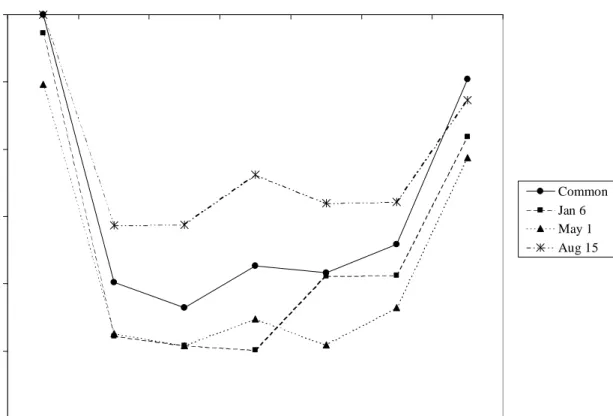
To highlight the importance of allowing for different effects for each class of public holiday, Figure 6 displays the estimated decrease of the load on the day of the holiday. Although some particular coefficients could be restricted to take the same value, as a whole the response varies in magnitude and shape. The estimated standard deviation for each estimator is about 0.5%, and broadly speaking all the differences between estimated responses above 1% are statistically significant.
Temperature effects
Meteorological variables play a leading role in the model, especially temperature. In this brief review we focus on the response to the daily maximum temperature and assume for simplicity that the other weather variables induce no additional effects on the load. The daily maximum temperature for mainland Spain is computed as a weighted average of the maximum temperatures recorded between 6 A.M. and 6 P.M. at ten observatories that represent different climatic regions; within a typical year it varies from a low of 8°C to a high of 34°C.
The estimated relation between load and temperature is highly complex for a number of reasons. On a priori grounds, the literature suggests that it is non-linear, U-shaped as long as there is enough variation of temperatures in the sample (Engle et al,
1986). The response is asymmetric, in the sense that a one-degree increase when the temperature is high and a one-degree decrease when the temperature is low need not have the same impact on the load (Valor et al, 2001). The relation differs for working
and nonworking days, as heating and cooling systems equipment and operation are very different in workplaces and private residences (Smith, 2000); it also changes with the time of the year (Hyde and Hodnett, 1997). There is a dynamic effect, as the load at t does not depend solely on the temperature at t but also on the temperatures at the previous days (Lecomte and Warren, 1981). Exhaustion effects may appear because of the limited capacity of existing electricity appliances, so there is no further increase in electricity consumption when the temperature exceeds some saturation level (Henley and Peirson, 1997).
The particular shape of the response is specific for each set of data and issues like the degree of nonlinearity, the order of the dynamics, or the presence and location of the saturation levels, for instance, must be empirically determined. In what follows
we focus on the main characteristics of the estimated relation as it is currently used to forecasting the load. Further details on the modelling strategy can be found in Cancelo and Espasa (1996).
The response to the maximum temperature has two branches, one for temperatures below 20°C and one for temperatures higher than 24°C. The interval from 20°C to 24°C is a comfort zone of moderate temperatures with no effect on electricity consumption. The general expression of the response to low temperatures is given by:
) 7 ( 20 HDDS 14 HDDS 11 HDDS 9 HDDS 5 0 i i t i t 0 t 0 t 0
∑
= − π + γ + β + α with ) 8 ( 9 max T if 9 x x max T 9 if max T x x max T if 0 HDDSx t t t t t < − < < − > =where Tmaxt denotes the observed maximum temperature and HDDSxt is a heating degree-days variable with reference temperature x and saturation level 9°C.
Expression (7) captures the basic shape of the relation for temperatures below 20°C, but it was found that its magnitude depends on the time of the year and, in some seasons, on the day of the week. Two seasons are distinguished, which will be referred to as summer and non-summer or rest of the year. In the non-summer season the response is different for normal weekdays and for weekends / special weekdays. In the summer season the impact does not depend on the day of the week and the response is much simpler: temperatures below 16°C are seldom observed and the dynamics go from t to t-2, so the only non-zero coefficients in (7) are π0, π1 and π2.
At the other branch of the curve, the response to high temperatures is given by ) 9 ( 24 CDDS 2 0 i i t i
∑
= − ωwhere CDDS24t is a cooling degree-days variable with threshold 24°C and saturation level 33°C: ) 10 ( 33 max T if 9 33 max T 24 if 24 max T 24 max T if 0 24 CDDS t t t t t > < < − < =
Temperatures above 24°C only affect the load in the summer season, and there are no differences between normal weekdays and weekends / special days. The response increases linearly from 24°C up to 33°C and remains constant above that level. The load at t depends on the observed temperatures at t, t-1 and t-2.
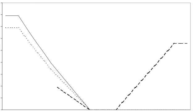
To summarize the estimated effects, Figure 7 displays the long-run gain for each temperature value. The long-run gain for Tmax=Tmax* is defined as the percent increase of the daily load at day t assuming that the temperature keeps constant at Tmax* for all the relevant lags in equations (7) and (9), with respect to the consumption that would have been registered if the temperature had been within the interval 20°C to 24°C. As an example, the gain for Tmax=26°C is equal to 2.48%: it means that if the observed maximum temperature in days t-2, t-1 and t is 26°C, the daily consumption at t will be 2.48% higher than if the temperature had been within the interval 20°C to 24°C during that period.
INSERT FIGURE 7 HERE
4. FORECAST PERFORMANCE DURING 2006
In Section 3 it was stated that there are two types of forecasts of special interest to REE, several days ahead predictions for daily data, and one day ahead hourly forecasts. Accordingly, forecast accuracy should be assessed in terms of their errors, so in this section we discuss the performance of the models with regard to both activities throughout 2006.
4.1 Prediction up to ten days ahead using the daily model
Daily forecasts are used to set up the weekly network outage plan. They are computed by the middle of the week, usually on Wednesday morning with information up to Tuesday, for the seven-day period beginning the following Saturday. The relevant lead times go from 4 to 10 days ahead, although there are some minor modifications as the origin of the forecast changes when a public holiday falls on Wednesday (four times in 2006). We ignore that for simplicity and act as if there were a one-to-one relation between the day of the week and the lead time. The forecasts are based on model parameters that were estimated using daily data from January 1, 1993 to March 31, 2005 (4473 observations); no reestimation was performed during 2006.
Two types of errors are computed, historical errors and model errors. By historical errors we mean real time errors, i.e., the errors that were actually observed. They arise either because of model misspecification or as a consequence of the errors made in forecasting meteorological variables; temperature forecasts are highly accurate for horizons up to three or four days, but they deteriorate as the lead time goes further. Hence, and in order to assess the influence of meteorological predictions, the load forecasts were recalculated by inserting the true values of the meteorological variables in the model, and the resulting errors are referred to as strict model errors.
Box-plots of the observed absolute percentage errors (APE) for historical errors are displayed in Figure 8. Table 1 reports mean absolute percentage errors (MAPE) for historical errors and model errors. It is well known that each set of data deserves particular consideration, and no general indications on how effective a forecasting procedure is can be given unless an explicit comparative evaluation is carried out on the same time series. In spite of that, the real time performance of the model looks satisfactory, in the sense that the errors are within the bounds that secure the electricity
supply security and quality. In the full year the MAPEs of the historical errors are always below 2.9% even for lead times of ten days ahead. They increase with the lead time, as expected, although there is some evidence that the forecasts are slightly worse on Sundays.
INSERT FIGURE 8 HERE INSERT TABLE 1 HERE
Using temperature predictions instead of true values has no perceptible effect on Saturday's forecasts. From Sunday on part of the actual error in forecasting the daily load is due to unsatisfactory temperature predictions, and that part increases with the lead time. The MAPEs of the model errors increase with the lead time too, but do not exceed 2% in any case. Model errors confirm that the forecasting performance is less satisfactory on Sunday than on weekdays.
To assess the performance by time of the year the database of errors was split in two parts, summer and rest-of-the-year. Table 1 indicates that the forecasts deteriorate during the summer months, especially in weekdays. Errors in forecasting temperature have to do with this deterioration for the longest horizons, but it basically reflects a weakness of the model and not of any of its inputs. The most important errors concentrate on August, a major period of vacation in mainland Spain: according to official estimates, the industrial production index fell by more than 30% in August 2005 due to seasonal effects. The model includes some dummy variables to capture the effects of the vacation on the load, but for the moment the results have not been as satisfactory as for the rest of the year.
As for the type of day, it is not straightforward to compare the forecasting performance for weekdays that are normal days, weekdays that are special days and weekends, because of the changing lead time. In order to give some indication on this
issue, we concentrated on weekdays and separated normal days (214 observations in the forecasting period) from special days (46 observations). For historical errors the MAPE is 2.34% for normal weekdays and 2.63% for special weekdays, while for model errors it is equal to 1.65% and 2.06%, respectively.
Decision makers are especially concerned about large errors, as they entail major rises in costs due either to unnecessary start-ups and energy purchases, or to very marginal scheduling that increases the likelihood of failures or equipment damage. There is not a general agreement about what a large error is, as each organization determines its own acceptable limit given its activities and aims. From the point of view of a utility, for instance, that limit heavily depends on its characteristics and operational features, but it also varies according to the day of the week and the hour of the day, the type of load (hourly, daily or peak), etc.
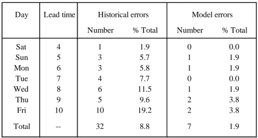
For simplicity, in this paper we assume a constant limit equal to 5%, so any error above that level in absolute value is termed a large error. This is a rough estimate that is often used at REE and has also been suggested as an adequate benchmark in the literature; see for instance Ranaweera et al (1997). Table 2 shows that in 2006 there
were 32 large historical errors (out of 365, or 8.8%). The number of large errors increases with the lead time, as expected. Interestingly, most of them are caused by errors in predicting the weather variables: when model errors are considered there are only 7 large errors, less than 2% of the total.
INSERT TABLE 2 HERE
4.2 Forecasting the hourly load for the next-day dispatch schedule
The hourly forecasts that determine the final dispatch schedule for the next day constitute the second set of critical forecasts for REE. Such forecasts are computed every day and the lead time is always one day. Contrary to the previous exercise, now
the lead time is constant and the origin changes along the week. The models are reestimated daily, so the forecast for day t is based on parameters that were estimated using data from January 1, 2001 to the last available observation.
Figure 9 displays box-plots of the historical hourly absolute percentage errors of the forecasts for the next day that were made public at REE's web page during 2006. They refer to 365 consecutive days with no exceptions, no corrections for public holidays, vacation periods, cold snaps, unexpected events, etc., other than those implemented in the models, and no supplementary subjective adjustments by the control operator or any other expert. Table 3 reports the related hourly mean absolute percentage errors. When no differences are made by day of the week the MAPE remains below 2% for all 24 hours. It takes its lowest values at late night hours and early in the morning, up to 8 A.M.; within this period it lies between 1.3% and 1.5%. Next it increases to about 1.6% in the first half of the business hours, from 10 A.M. to 3 P.M., and further to more than 1.7% from 4 P.M. to 8 P.M. A closer inspection of Table 3 reveals that this pattern of intraday evolution is not stable as it changes according to the type of day. In the beginning of the week, from Sunday to Tuesday, the maximum MAPE is attained by 9 A.M.-10 A.M., while on Saturdays it is not observed until 7 P.M.
INSERT FIGURE 9 HERE INSERT TABLE 3 HERE
When the database of errors is split by day of the week it is found that the most difficult period to predict is Saturday afternoon (from 5 P.M. to 8 P.M.), followed by Sunday morning (from 9 A.M. to 11 A.M.) and Monday morning (from 10 A.M. to 12 P.M.). Saturday afternoon behaves like a Sunday in some aspects and like a weekday in regard to commercial activities, especially retail trading, and that duality increases
forecast uncertainty to its maximum. In any case there are only 13 values of the MAPE higher than 2% (out of 168, or 7.7%), and none above 2.5%.
Table 4 reports MAPEs computed separately by time of the year and by type of day. Contrary to what was found in daily forecasting, the hourly models perform better in the summer season for almost all hours, although the difference is higher early in the morning. With regard to the types of day, there are differences in the magnitude of the errors among normal weekdays, weekends and special weekdays. For normal weekdays MAPEs vary from 1.14% at 7 A.M. to 1.64% at 6 P.M. The intraday evolution is rather similar in weekends, but now the MAPEs range from a low of 1.40% at 7 A.M. to a high of 2.15% at 7 P.M. Finally, for weekdays that are special days the MAPES go from 1.39% at 4 A.M. to 2.90% at 5 P.M.
INSERT TABLE 4 HERE
Table 5 details the number of large errors (above 5% in absolute value) by day of the week. The total number is 218 out of 8760, or 2.5%. Large errors are more likely to occur from 5 P.M. to 8 P.M. and on weekends: almost one third is within that four-hour interval, and 44% are either on Sunday or Saturday. It should be noted, however, that the differences among the MAPEs reported in Table 3 are not due solely to these large observations, as the pattern of unpredictability remains roughly the same when the means are recalculated without considering the errors above 5%.
INSERT TABLE 5 HERE
To conclude this review of the forecasting performance of the hourly models, we assess its relative performance with respect to two benchmarks. Some years ago REE contacted two external organizations to develop alternative forecasting procedures; both of them are proprietary and we do not have permission to describe their details in this paper. The first alternative (benchmark 1) combines seasonal decomposition,
exponential smoothing and neural networks; it includes temperature as an explanatory variable, but does not make any allowance for special days. The second procedure (benchmark 2) combines seasonal ARIMA models and artificial neural networks, includes temperature variables, and models special days in an explicit way.
It was found that the existing models were more accurate than both benchmarks, so the latter were discarded for on-line operation. But it was also decided that the two benchmarks would be used off-line to help in monitoring the performance of the preferred models. For doing so, hourly forecasts are computed from the three methods at the same time and based on the same information, so that they are fully comparable. They are not comparable, however, to the true historical errors reported in previous tables for a variety of reasons: they are usually computed on normal weekdays at 10 A.M. for the entire next day, so in practice they are closer to a two-day ahead forecast; on Friday the full weekend plus Monday are forecasted; when there is a public holiday, the forecasts are computed at the previous day up to the next working day; on vacation periods there are some missing data (39 full days in 2006); etc.
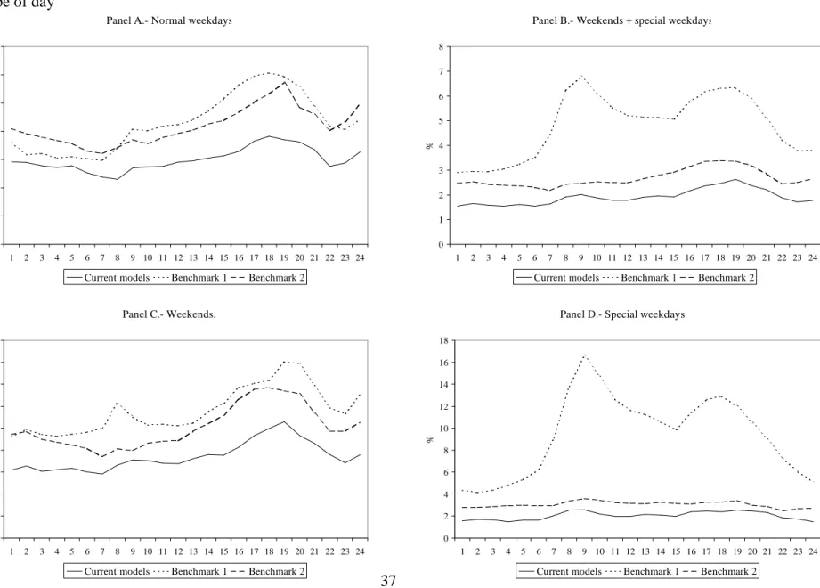
The results are summarized in Table 6 and Figure 10. Table 6 sketches the main features by focusing on daily figures. The forecasting performance of each method is measured by the daily MAPE and the number of daily errors above 5%. The daily MAPE is the average of the 24 hourly MAPEs; the number of large errors is the number of days with a daily absolute percentage error (APE) above 5%, daily APE being computed as the average of the 24 hourly APEs. The results are reported for the whole set of data and separately by type of day. In addition, Figure 10 compares the 24 hourly MAPEs for each type of day and gives a more detailed picture of the relative performance of the methods.
INSERT FIGURE 10 HERE
Table 6 and Figure 10 show that the current models outperform the benchmarks in all possible comparisons. They confirm that modelling special days is a major need in forecasting the load, compare the performance of benchmark 1 with respect to the two other procedures. With regard to the comparison between the current models and benchmark 2, it can be seen in Table 6 that the daily MAPEs are from 0.6% to 1% lower in the current models. Besides, in Figure 10 the four curves of the current models are always below the related curves of the second benchmark. Finally, it was noted in Table 4 that the forecasting performance of the current models is not as satisfactory for special days as it is for normal weekdays. The differences, however, are smaller for the current models than for benchmark 2, so it seems that the former are more successful in detecting the pattern of systematic variation of special days and in using it to improve the forecasts.
5. SUMMARY AND CONCLUSIONS
In this paper we have presented the experience of Red Eléctrica de España
(REE), the Spanish transmission system operator, in forecasting the electricity load. Adopting the point of view of a specific agent within the power system is one of the distinguishing features of the paper. It leads to making explicit the actual needs of the organization and the kind of information forecasts are asked to provide, and they both determine the way the forecasting activity should be approached and how it should be evaluated.
Even though there is a wide, systematic production of forecasts at specific moments of the day or the week at REE, there are two particular types of special interest: the daily forecasts that are calculated on Wednesday morning for the seven-day
period beginning on the following Saturday, which are used for outage planning; and every day's hourly forecasts to set up the final hourly dispatch schedule for the next day. Both categories are critical inputs for REE's activities, to the extent that forecasting success should be mainly assessed in terms of their errors. A point that has been stressed throughout the paper is that in applied forecasting we need to identify the needs of the particular agent, set up adequate devices specifically designed to meet such needs, and monitor performance by focusing on the errors that have significant economic impacts according to the activities of the organization.
The current forecasting system implemented at REE consists of one daily model to forecast the daily load up to ten days ahead, and 24 hourly models to compute hourly predictions for horizons up to three days. All the models share a common basic structure, although their parameters are allowed to adapt to the particular features of each time series.
The forecasting performance was evaluated by analyzing different types of errors for the year 2006. Mean absolute percentage errors for historical, real time daily forecasts ranged from 1.3% to 2.8% even for lead times of ten days ahead, and a significant part of the error was caused by errors in predicting the weather variables. There were 32 historical errors above 5% in absolute value, and only 7 were strict model errors. The forecasting performance in special weekdays is worse than in normal weekdays, although the difference between the MAPEs is small and indicates that the model has been quite successful in explaining most of the distortions induced by the occurrence of a special day.
In regard to the hourly forecasts for the next-day dispatch schedule, the MAPEs for historical errors were between 1.3% and 1.9% and there were 218 errors higher than
5%, 2.5% of the total. It was found that the most difficult period to predict is Saturday afternoon, as it behaves like a Sunday in some aspects and like a weekday in others.
The performance of the hourly models was compared to two different benchmarks. A distinguishing feature of this paper is that the benchmarks are competing methods acquired to external organizations to challenge the existing procedure and even to become the main forecasting devices. Nevertheless, the current models outperformed the benchmarks in all comparisons. In particular, the exercise showed that the major improvement in error reduction comes from understanding how the load reacts to special days, and integrating their influence together with weather variables' effects in a comprehensive model that captures the main determinants of the electricity load.
REFERENCES
Cancelo, J. R. & Espasa, A. (1996). Modelling and forecasting daily series of electricity demand. Investigaciones Económicas, XX, 359-376.
Cancelo, J. R. & Espasa, A. (2001). Using high-frequency data and time series models to improve yield management. International Journal of Services Technology and Management, 2, 59-70.
Chen, H., Cañizares, C. A. & Singh, A. (2001). ANN-based short-term load forecasting in electricity markets. Power Engineering Society Winter Meeting, IEEE, 2, 411-415.
Cottet, R. & Smith, M. (2003). Bayesian modeling and forecasting of intraday electricity load. Journal of the American Statistical Association, 98, 839-849.
Darbellay, G. A. & Slama, M. (2000). Forecasting the short-term demand for electricity. Do neural networks stand a better chance? International Journal of Forecasting, 16, 71-83.
Engle, R. F., Granger, C. W. J., Rice, J. & Weiss, A. (1986). Semiparametric estimates of the relation between weather and electricity sales. Journal of the American Statistical Association, 81, 310-320.
Espasa, A., Revuelta, J. M. & Cancelo, J. R. (1996). Automatic modelling of daily series of economic activity. In: A. Prat (Ed.), Proceedings in computational statistics COMPSTAT 1996. Heidelberg: Physica-Verlag, pp. 51-63.
Harvey, A. & Koopman, S. J. (1993). Forecasting hourly electricity demand using time-varying splines. Journal of the American Statistical Association, 88, 1228-1236.
Henley, A. & Peirson, J. (1997). Non-linearities in electricity demand and temperature: parametric versus non-parametric methods. Oxford Bulletin of Economics and Statistics, 59, 149-162.
Hippert, H. S., Pedreira, C. E. & Souza, R. C. (2001). Neural networks for short-term load forecasting: a review and evaluation. IEEE Transactions on Power Systems, 16, 44-55.
Hippert, H. S., Bunn, D. W. & Souza, R. C. (2005). Large neural networks for electricity load forecasting: are they overfitted? International Journal of Forecasting, 21, 425-434.
Hyde, O. & Hodnett, P. F. (1997). An adaptable automated procedure for short-term electricity load forecasting. IEEE Transactions on Power Systems, 12, 84-94.
Lamedica, R., Prudenzi, A., Sforna, M., Caciotta, M. & Orsolini Cencelli, V. (1996). A neural network based technique for short-term forecasting of anomalous load periods. IEEE Transactions on Power Systems, 11, 1749-1756.
Le Comte, D. M. & Warren, H. E. (1981). Modeling the impact of summer temperatures on national electricity consumption. Journal of Applied Meteorology, 20, 1415-1419.
Nevis, E. C., DiBella, A. J. & Gould, J. M. (1995). Understanding organizations as learning systems. Sloan Management Review, 36, 73-85.
Pardo, A., Meneu, V. & Valor, E. (2002). Temperature and seasonality influences on Spanish electricity load. Energy Economics, 24, 55-70.
Ramanathan, R., Engle, R., Granger, C. W. J., Vahid-Araghi, F. & Brace, C. (1997). Short-run forecasts of electricity loads and peaks. International Journal of Forecasting, 13, 161-174.
Ranaweera, D. K., Karady, G. G. & Farmer, R. G. (1997). Economic impact analysis of load forecasting. IEEE Transactions on Power Systems, 12, 1388-1392.
Schneider, A. M., Takenawa, T. & Schiffman, D. A. (1985). 24-Hour electric utility load forecasting. In: D. W. Bunn & E. D. Farmer (Eds.), Comparative models for electric load forecasting. New York: John Wiley & Sons, pp. 87-108.
Schultz. R. L. (1992). Fundamental aspects of forecasting in organizations. International Journal of Forecasting, 7, 409-411.
Smith, M. (2000). Modeling and short-term forecasting of New South Wales electricity system load. Journal of Business & Economic Statistics, 18, 465-478.
Soares, L. J. & Souza, L. R. (2006). Forecasting electricity demand using generalized long memory. International Journal of Forecasting, 22, 17-28.
Taylor, J. W. (2003). Short-term electricity demand forecasting using double seasonal exponential smoothing. Journal of the Operational Research Society, 54, 799-805.
Taylor, J. W., de Menezes, L. M. & McSharry, P. E. (2006). A comparison of univariate methods for forecasting electricity demand up to a day ahead. International Journal of Forecasting, 22, 1-16.
Valor, E., Meneu., V. & Caselles, V. (2001). Daily air temperature and electricity load in Spain. Journal of Applied Meteorology, 40, 1413-1421.
Figure 1.- Monthly electricity consumption in mainland Spain: original series and trend computed with a Hodrick-Prescott filter with λ=14,400
10000 14000 18000 22000 26000 1993 1994 1995 1996 1997 1998 1999 2000 2001 2002 2003 2004 2005 2006 G W h
Figure 2.- Daily electricity load in 2005 400 500 600 700 800 900
Jan Feb Mar Apr May Jun Jul Aug Sep Oct Nov Dec
G
W
Figure 3.- Intraday electricity load patterns
Panel A.- Winter season 1/30/2005 - 2/12/2005 .
15 20 25 30 35 40 45 S M T W T F S S M T W T F S G W h
Panel B.- Summer season 7/10/2005 - 7/23/2005 .
15 20 25 30 35 40 45 S M T W T F S S M T W T F S G W h
Figure 4.- Effect of a public holiday on load
Panel A.- Daily load 10/3/2004 - 10/23/2004 .
400 450 500 550 600 650 700 S M T W T F S S M T W T F S S M T W T F S G W h Oct 12
Panel B.- Hourly load 10/10/2004 - 10/23/2004 .
15 20 25 30 35
Sun Mon Tue Wed Thu Fri Sat
G
W
h
10/10/2004 - 10/16/2004 10/17/2004 - 10/23/2004
Panel D.- Hourly load 10/9/2005 - 10/22/2005 .
15 20 25 30 35
Sun Mon Tue Wed Thu Fri Sat
G
W
h
10/9/2005 - 10/15/2005 10/16/2005 - 10/22/2005 Panel C.- Daily load 10/2/2005 - 10/22/2005 .
400 450 500 550 600 650 700 S M T W T F S S M T W T F S S M T W T F S G W h Oct 12
Figure 5.- Daily load and maximum temperature in 2005 400 500 600 700 800 900 0 5 10 15 20 25 30 35 40 Degrees Celsius G W h
Figure 6.- Estimated decrease of the daily load on a public holiday -30 -25 -20 -15 -10 -5 0
Sun Mon Tue Wed Thu Fri Sat
%
Common Jan 6 May 1 Aug 15
Figure 7.- Long-run gain of the maximum temperature: percent increase of the daily load with respect to the load for temperatures within the interval 20°C to 24°C
0 2 4 6 8 10 12 14 16 18 7 8 9 10 11 12 13 14 15 16 17 18 19 20 21 22 23 24 25 26 27 28 29 30 31 32 33 34 35 Degrees Celsius %
Figure 8.- Box-plots of the historical, real time Absolute Percentage Errors (APE) in daily forecasting for the network outage plan
Figure 9.- Box-plots of the historical, real time Absolute Percentage Errors (APE) in hourly forecasting for the next-day dispatch schedule
Sat Sun Mon Tue Wed Thu Fri 0 2 4 6 8 10 12 14 16 1 2 3 4 5 6 7 8 9 10 11 12 13 14 15 16 17 18 19 20 21 22 23 24 0 2 4 6 8 10 12 14
Figure 10.- Forecasting comparison among the current hourly models and two third-party benchmarks: hourly mean absolute percentage errors by type of day
Panel A.- Normal weekdays.
0.0 0.5 1.0 1.5 2.0 2.5 3.0 3.5 1 2 3 4 5 6 7 8 9 10 11 12 13 14 15 16 17 18 19 20 21 22 23 24 %
Current models Benchmark 1 Benchmark 2
Panel B.- Weekends + special weekdays.
0 1 2 3 4 5 6 7 8 1 2 3 4 5 6 7 8 9 10 11 12 13 14 15 16 17 18 19 20 21 22 23 24 %
Current models Benchmark 1 Benchmark 2
Panel C.- Weekends. 0.5 1.0 1.5 2.0 2.5 3.0 3.5 4.0 4.5 %
Panel D.- Special weekdays.
2 4 6 8 10 12 14 16 18 %
Table 1.- Mean absolute percentage errors (MAPE) in daily forecasting
Table 2.- Absolute percentage errors higher than 5% in daily forecasting
Day Lead time
All Non-summer Summer Difference All Non-summer Summer Difference
Sat 4 1.34 1.33 1.35 0.02 1.35 1.32 1.40 0.08 Sun 5 1.97 2.03 1.86 -0.17 1.74 1.80 1.62 -0.18 Mon 6 2.13 2.16 2.07 -0.09 1.53 1.53 1.52 -0.01 Tue 7 2.06 1.79 2.63 0.84 1.53 1.18 2.26 1.08 Wed 8 2.36 1.95 3.19 1.24 1.72 1.32 2.54 1.22 Thu 9 2.59 2.08 3.61 1.53 1.81 1.45 2.58 1.13 Fri 10 2.82 2.23 3.95 1.72 2.01 1.74 2.53 0.79
Historical errors Model errors
Day Lead time
Number % Total Number % Total
Sat 4 1 1.9 0 0.0 Sun 5 3 5.7 1 1.9 Mon 6 3 5.8 1 1.9 Tue 7 4 7.7 0 0.0 Wed 8 6 11.5 1 1.9 Thu 9 5 9.6 2 3.8 Fri 10 10 19.2 2 3.8 Total -- 32 8.8 7 1.9 Model errors Historical errors
Table 3.- Mean absolute percentage errors in hourly forecasting: all days and details by day of the week
Hours All days
Sun Mon Tue Wed Thu Fri Sat
1 A.M. 1.34 1.55 1.28 1.47 1.36 1.47 1.04 1.23 2 A.M. 1.37 1.70 1.05 1.52 1.33 1.45 1.17 1.37 3 A.M. 1.35 1.78 1.08 1.66 1.33 1.33 1.06 1.23 4 A.M. 1.35 1.80 1.19 1.61 1.23 1.28 1.02 1.32 5 A.M. 1.39 1.80 1.22 1.69 1.41 1.26 0.99 1.34 6 A.M. 1.31 1.61 1.17 1.51 1.34 1.30 0.99 1.25 7 A.M. 1.33 1.47 1.24 1.53 1.33 1.22 1.18 1.33 8 A.M. 1.45 1.64 1.56 1.52 1.39 1.30 1.28 1.46 9 A.M. 1.66 2.03 1.87 1.78 1.66 1.42 1.31 1.52 10 A.M. 1.63 2.08 2.14 1.57 1.60 1.43 1.32 1.26 11 A.M. 1.60 2.06 2.01 1.46 1.55 1.45 1.40 1.24 12 P.M. 1.60 1.89 2.02 1.52 1.53 1.45 1.52 1.26 1 P.M. 1.61 1.79 1.86 1.52 1.59 1.49 1.58 1.41 2 P.M. 1.62 1.77 1.78 1.57 1.58 1.52 1.60 1.50 3 P.M. 1.63 1.79 1.75 1.54 1.57 1.65 1.55 1.53 4 P.M. 1.77 1.91 1.95 1.60 1.63 1.76 1.74 1.77 5 P.M. 1.91 1.97 1.97 1.68 1.88 1.72 2.05 2.09 6 P.M. 1.90 1.82 1.81 1.71 2.03 1.65 1.95 2.32 7 P.M. 1.85 1.91 1.66 1.66 2.08 1.56 1.69 2.39 8 P.M. 1.74 1.84 1.67 1.68 1.89 1.55 1.53 2.03 9 P.M. 1.63 1.93 1.70 1.49 1.81 1.36 1.39 1.72 10 P.M. 1.40 1.66 1.57 1.22 1.47 1.09 1.16 1.60 11 P.M. 1.39 1.40 1.59 1.21 1.62 1.21 1.15 1.57 12 A.M. 1.55 1.80 1.61 1.44 1.67 1.24 1.35 1.73 All hours 1.56 1.79 1.62 1.55 1.58 1.42 1.38 1.56
Table 4.- Mean absolute percentage errors in hourly forecasting: details by time of the year and types of day Hours
Non-summer Summer Weekdays, normal Weekends + Weekends Weekdays, special
Weekdays, special 1 A.M. 1.39 1.25 1.28 1.44 1.40 1.54 2 A.M. 1.44 1.23 1.25 1.54 1.54 1.55 3 A.M. 1.48 1.10 1.23 1.53 1.51 1.56 4 A.M. 1.47 1.11 1.24 1.51 1.56 1.39 5 A.M. 1.55 1.07 1.28 1.54 1.57 1.49 6 A.M. 1.47 0.99 1.17 1.52 1.43 1.70 7 A.M. 1.47 1.05 1.14 1.59 1.40 2.03 8 A.M. 1.56 1.24 1.20 1.80 1.55 2.39 9 A.M. 1.81 1.35 1.38 2.06 1.78 2.71 10 A.M. 1.76 1.37 1.40 1.95 1.67 2.59 11 A.M. 1.67 1.46 1.40 1.88 1.65 2.39 12 P.M. 1.66 1.47 1.41 1.86 1.58 2.51 1 P.M. 1.66 1.51 1.42 1.87 1.61 2.48 2 P.M. 1.70 1.46 1.42 1.90 1.64 2.49 3 P.M. 1.70 1.48 1.43 1.90 1.66 2.44 4 P.M. 1.88 1.55 1.49 2.16 1.84 2.88 5 P.M. 2.02 1.67 1.64 2.29 2.03 2.90 6 P.M. 1.98 1.73 1.64 2.26 2.07 2.71 7 P.M. 1.94 1.67 1.53 2.31 2.15 2.67 8 P.M. 1.82 1.58 1.49 2.10 1.94 2.47 9 P.M. 1.69 1.50 1.37 1.99 1.82 2.37 10 P.M. 1.46 1.27 1.17 1.72 1.63 1.94 11 P.M. 1.38 1.41 1.26 1.59 1.48 1.82 12 A.M. 1.55 1.55 1.41 1.74 1.76 1.69 All hours 1.65 1.38 1.36 1.84 1.68 2.20
Table 5.- Number of absolute percentage errors higher than 5% in hourly forecasting
Hours All days
Sun Mon Tue Wed Thu Fri Sat
1 A.M. 4 1 0 0 1 1 0 1 2 A.M. 4 2 0 0 0 1 0 1 3 A.M. 5 3 0 1 0 1 0 0 4 A.M. 5 4 0 0 0 1 0 0 5 A.M. 7 4 0 0 1 1 0 1 6 A.M. 3 1 0 0 0 1 0 1 7 A.M. 5 1 0 1 1 1 0 1 8 A.M. 9 2 0 1 1 2 1 2 9 A.M. 13 2 1 2 2 2 1 3 10 A.M. 11 4 0 2 2 2 0 1 11 A.M. 8 5 0 0 1 1 0 1 12 A.M. 9 4 2 1 1 0 1 0 1 P.M. 10 3 2 1 1 1 1 1 2 P.M. 12 3 1 3 1 1 2 1 3 P.M. 9 3 2 2 1 0 1 0 4 P.M. 10 2 2 2 1 0 3 0 5 P.M. 20 3 6 3 1 1 4 2 6 P.M. 16 1 4 2 1 1 3 4 7 P.M. 18 1 2 2 2 1 3 7 8 P.M. 17 2 2 3 2 1 1 6 9 P.M. 5 0 0 1 0 0 1 3 10 P.M. 5 0 0 1 0 0 1 3 11 P.M. 7 1 0 1 1 0 1 3 12 P.M. 6 1 0 1 1 0 1 2 All hours 218 53 24 30 22 20 25 44
Table 6.- Forecasting comparison among the current hourly models and two third-party benchmarks: daily mean absolute percentage errors and number of errors above 5% by type of day
Note: The daily MAPE is computed as the average of the 24 hourly MAPEs; the number of errors above 5% is based on the daily average percentage error, which is computed as the average of the 24 hourly APEs for that day.
Types of day Number of observations
Current models Benchmark 1 Benchmark 2 Current models Benchmark 1 Benchmark 2
All days 326 1.66 3.21 2.32 2 39 26
Weekdays, normal 196 1.50 2.15 2.09 0 8 10
Weekends + weekdays, special 130 1.91 4.81 2.68 2 31 16
Weekends 92 1.86 2.91 2.52 2 10 9
Weekdays, special 38 2.04 9.42 3.06 0 21 7
Number of errors above 5% Mean Absolute Percentage Errors (MAPE)