206
STEADY STATE VORTEX STRUCTURE OF LID DRIVEN FLOW INSIDE SHALLOW SEMI ELLIPSE CAVITY
M. S. Idris1 , M. A. M. Irwan2 and N. M. M. Ammar1 1
Computational Analysis Group, Faculty of Mechanical Engineering,
Universiti Malaysia Pahang (UMP), 26600 Pekan, Pahang, Malaysia Email: [email protected]
2
Faculty of Mechanical Engineering,
Universiti Teknikal Malaysia Melaka (UTeM), 76100, Durian Tunggal, Melaka, Malaysia
ABSTRACT
In this paper, the lid driven cavity flow inside semi-ellipse shallow cavity was simulated using stream function vorticity approach emphasizing non-uniform grid method. Three aspect ratio of 1/4, 1/3 and 3/8 were simulated using laminar flow conditions (range of Reynolds numbers of 100-2000). Primary and secondary vortexes were extensively monitored through centre vortex location, streamlines pattern and peak stream function value. Secondary vortex developed at Re 1500 for the aspect ratio of 1/4 while the secondary vortex formed at earlier Reynolds number of 1000 for the aspect ratio of 1/3 and 3/8. The size of secondary vortex increases as Reynolds number increases. The similar trends can be observed the differences between primary vortex separation angle and reattachment angle. For the entire streamline pattern, many primary vortex centre locations situated at the right side of the cavity.
Keywords: Semi-ellipse, lid driven cavity flow, DNS, non-uniform.
INTRODUCTION
The lid driven cavity flow is one of the well-known fluid problems which is solved numerically and many considered this problem attractive and seductive. The latter consideration is quite because of the lid driven cavity flow not depleting over the years. There are many usage of lid driven cavity flow solution in the powder technology, mixing, segregating and formation of eddies (Kosinski et al., 2009). This is due to the mathematical part and fluids physics contained by the problem itself. Nonetheless, the lid driven cavity flow was prepared by Ghia et al. (1982). Other papers such as (Barragy and Carey, 1997, Botella and Peyret, 1998) have embarked a new paradigm for lid driven cavity flow solution. Despite that, many researchers focus on the numerical solution of top driven lid square cavity which reflects the mathematical part. For instance the lid driven cavity flow of square cavity with top lid moving is solved using finite different method (Weinan and Liu, 1996), finite volume method (Peri et al., 1988), Lattice Boltzmann method (Azwadi and Idris, 2010, Zin and Sidik, 2010), Chebyshev projection method (Botella, 1997) and spectral method. There are other types such as two driven side (Albensoeder et al., 2001) and even four sided driven boundary (Wahba, 2009) while others study the effect of shallow cavity (Zdanski et al., 2003), deep cavity (Cheng and Hung, 2006) and vorticity boundary condition (Weinan
207
and Liu, 1996). Even so, these research studies only focused on the rectangular cavity. Several scientists unbound themselves from adhering to rectangular cavity such as triangular cavity (Li and Tang, 1996, Ribbens, 1994, Jyotsna and Vanka, 1995, Erturk and Gokcol, 2007), trapezoidal cavity (McQuain et al., 1994, Zhang et al., 2010) and semicircular cavity (Mercan and Atalik, 2009, Chang and Cheng, 1999, Cheng and Chen, 2005). There are also real experiments on lid driven cavity flow (Koseff and Street, 1984a; Koseff and Street, 1984b; Prasad and Koseff, 1989). According to the authors’ extent of literature, there is a little information regarding lid driven cavity flow inside semi-elliptical boundary due to complexity of boundary. Therefore, this research will be conducted to provide the physical fluid behaviour and numerical result of lid driven cavity flow inside shallow semi ellipse cavity. The aspect ratio is chosen rather than eccentricity due to inability of eccentricity to distinguish between shallow or deep semi ellipses. There are three aspect ratio used for the simulation, which are 1/4, 1/3 and 3/8. Aspect ratio of 1/2 is not considered because of this value is equivalent to a semicircular cavity. For each aspect ratio, five Reynolds numbers (Re ) of 100, 500, 1000, 1500 and 2000 are simulated to monitor the behaviour of vortexes, vortex centre location value and stream function peak value as well as separation angles.
GOVERNING EQUATIONS AND NUMERICAL FORMULATION
Basically, this study was conducted with the emphasis of stream function vorticity approach. For this research, there are main equations with few auxiliary equations. These main equations are vorticity transport equation (1) and vorticity equation in term of stream function (2). These equations are in dimensionless form and all parameters are independent.
+ + = 1 ²+ ² (1)
² + ² (2)
As for the discretization method, explicit first order upwind scheme for temporal derivative and central finite difference for spatial derivative of non-uniform grid were utilized to obtain the numerical simulation. Special formulation for spatial derivative is implemented to mimic the curvilinear shape of the elliptical boundary. The special formulation was introduced and the formulation of first and second order derivative of non-uniform spatial grid approximation was proven more effective than previous non uniform grid equations, those were implemented and represent by Eq. (3-4) (Veldman and Rinzema, 1992) and for the physical formulation, the collocated nodes of non-uniform grid size are presented in Figure 1.
( ( ) (3) ² ² 2 ( ) ) 2 ( ) + 2 (( ) ) (4)
208
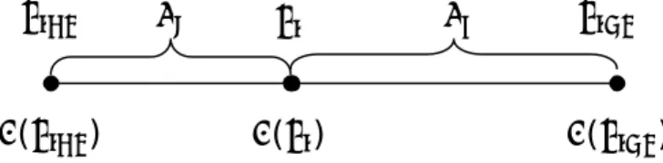
Figure 1. One dimensional non-uniform grid.
BOUNDARY DISCRETIZATION
The boundary of semi-ellipse cavity is very crucial especially at the bottom part with grid 14 × 7 as shown in Figure 2. When the grid spacing of actual 128 ×128 is to be presented as cavity model, the special spacing arrangement is difficult to make viewable. For the model of the semi-elliptic cavity, the mesh is unique whereas the grid spacing is different from each other. These spacing needs to be implemented to facilitate the curvature shape of the bottom cavity, which adopts the curvature of an isosceles triangle cavity. According to the Figure 2, the length of the lid, L (top boundary) is maintained at unity while the cavity height (H) change for various shallow aspect ratio (H/L or AR) of 1/4, 1/3 and 3/8. Hence, the irregular spacing of grid should be compensating the non-uniform equation for the derivatives terms.
Figure 2. Semi-ellipse cavity model.
RESULTS AND DISCUSSION
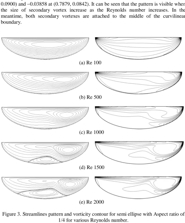
The grid independent tests were performed for 30 × 30, 60 × 60, 100 × 100 and 128 × 128. The obtained results indicate that the satisfactory result of streamlines pattern, location of primary and secondary vortex centre together with the value of peak stream function at grid value of 60 × 60. However, the 128 × 128 is considered to use although at the expense of time for better accuracy. Figure 3 shows the streamline pattern at the left and the vorticity contour on the right. This aspect ratio resembled the depth of semi ellipse cavity ratio to length of lid. For Re < 1500, the secondary vortex is absent which leave the primary vortex alone. Nevertheless, the centre of primary vortex changes from the centre cavity to the left of cavity as the Reynolds number increase. Table 1 is filled with the location of centre vortex and stream function value, both for primary and secondary vortex for aspect ratio of 1/4. The changes of vortex centre are significant in horizontal direction whereas the values are 0.5490, 0.7357 and 0.7464. On the counterpart, small changes of primary vortex centre in the vertical direction as the three values are 0.8420, 0.8420 and 0.9000. Meanwhile for Re 1500 and 2000, the secondary
209
vortex was developed whereas the location for the secondary vortexes are (0.5123, 0.1933) and (0.5123, 0.1723). The peak value of stream function are and 0.00096 and 0.00213. On the other hand, the stream function value of the primary vortex together with each location for Re 1500 and 2000 are 0.03983 at (0.7674, 0.0900) and 0.03858 at (0.7879, 0.0842). It can be seen that the pattern is visible when the size of secondary vortex increase as the Reynolds number increases. In the meantime, both secondary vortexes are attached to the middle of the curvilinear boundary. (a) Re 100 (b) Re 500 (c) Re 1000 (d) Re 1500 (e) Re 2000
Figure 3. Streamlines pattern and vorticity contour for semi ellipse with Aspect ratio of 1/4 for various Reynolds number.
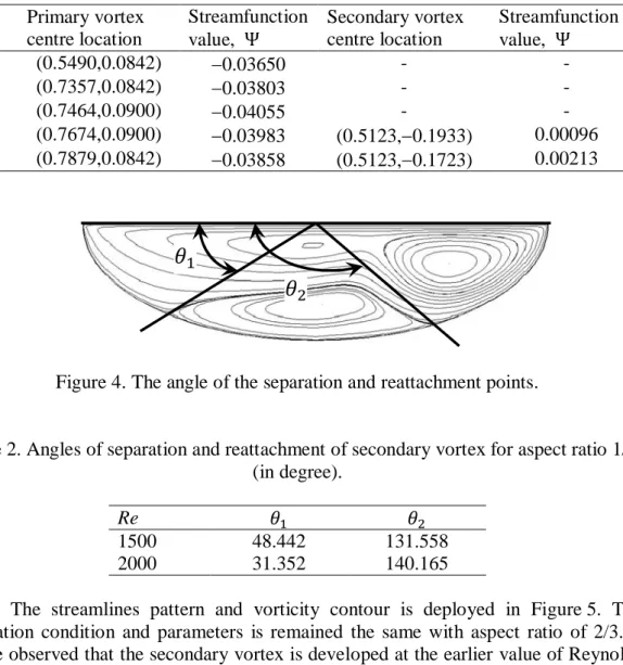
The condition of secondary vortex attachment and separation towards the curvilinear body is extracted from simulation results. The sketch for the angles is shown in Figure 4. The angles are calculated counter clockwise from the left side of cavity to the right side of cavity where represents the attachment angle of the secondary vortex toward the curvilinear boundary and represents the angle of separation for secondary vortex from the curvilinear boundary. These angles of attachment and separation are then compiled inside Table 2. It can be seen that the secondary vortex attached at the
210
angle of 48.442º and detached from the curvilinear boundary at the angle of 131.55º for Re of 1500. Meanwhile, for Re of 2000, the secondary vortex attached at the earlier angle of 31.352º and separates from the curvilinear boundary at angle of 140.165º. These angles are influenced by the size of the secondary vortex itself. It can be observed that the attachment angle decreases while the separation angle increases as the Reynolds number increase for the secondary vortex. For the vorticity contour, significant changes can be observed at the right side of the cavity as the centre of primary vortex located around this area.
Table 1. The primary and secondary vortex centre location and stream function values for aspect ratio of 1/4 with various Reynolds number.
Re Primary vortex centre location Streamfunction value, Secondary vortex centre location Streamfunction value, 100 (0.5490,0.0842) 0.03650 - - 500 (0.7357,0.0842) 0.03803 - - 1000 (0.7464,0.0900) 0.04055 - - 1500 (0.7674,0.0900) 0.03983 (0.5123, 0.1933) 0.00096 2000 (0.7879,0.0842) 0.03858 (0.5123, 0.1723) 0.00213
Figure 4. The angle of the separation and reattachment points.
Table 2. Angles of separation and reattachment of secondary vortex for aspect ratio 1/4 (in degree).
Re
1500 48.442 131.558
2000 31.352 140.165
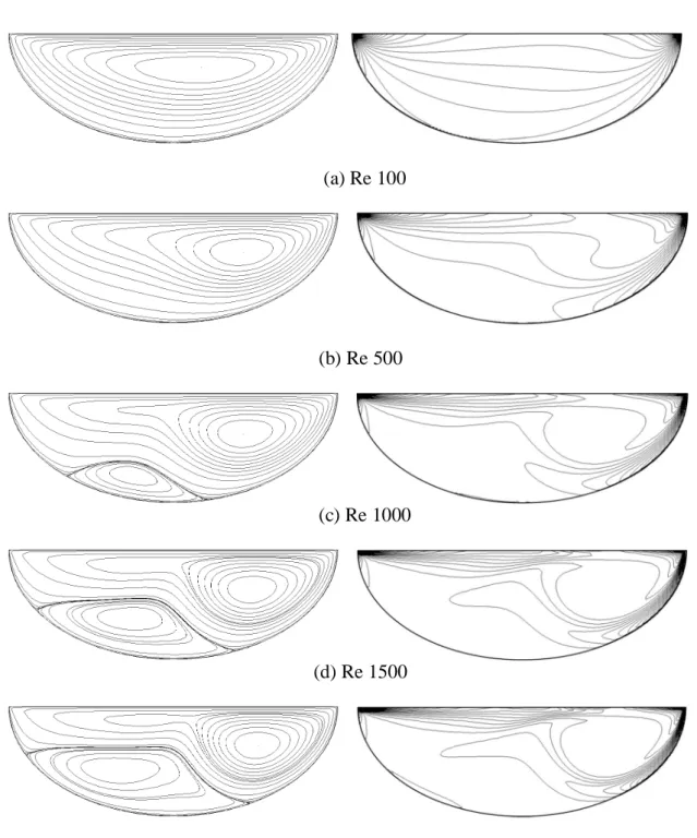
The streamlines pattern and vorticity contour is deployed in Figure 5. The simulation condition and parameters is remained the same with aspect ratio of 2/3. It can be observed that the secondary vortex is developed at the earlier value of Reynolds number 1000, the secondary vortex appear only for Reynolds number 1500. It can be noted that as the Reynolds number increase, the size of secondary vortex also increase. This condition is obvious for Reynolds number 1000 till 2000. The primary and secondary vortex centre location and stream function values for aspect ratio 1/3 with various Reynolds number are listed in Table 3. Primary vortex centre location shows obvious changes as the horizontal value move to left of cavity as the Reynolds number increase while for vertical value, most of the value settled at 0.1200 below the moving boundary. For the stream function, for Reynolds number 100 and 500, the value seems
211
to be increasing. However, for Reynolds number 1000, 1500 and 2000, the stream function magnitude decreases from 0.05291 to 0.05005 due to the appearance and the size of the secondary vortex which counter the primary vortex. On the other hand, the stream function value at the peak increased from 0.00082 to 0.00505 for the secondary vortex when the Reynolds number increased from 1000 to 2000. As for the location of the secondary vortex centre, it steadily moves downward the cavity when the Reynolds number increases. (a) Re 100 (b) Re 500 (c) Re 1000 (d) Re 1500 (e) Re 2000
Figure 5. Streamlines pattern and vorticity contour for semi ellipse with aspect ratio of 1/3 for various Reynolds number.
212
Table 3. The primary and secondary vortex centre location and stream function values for aspect ratio 1/3 with various Reynolds number.
Re Primary vortex centre location Streamfunction value, Secondary vortex centre location Streamfunction value, 100 (0.5855, 0.2288) 0.04811 - - 500 (0.7138, 0.1200) 0.05257 - - 1000 (0.7138, 0.1276) 0.05291 (0.3786, 0.0864) 0.00082 1500 (0.7357, 0.1200) 0.05133 (0.3666, 0.2051) 0.00301 2000 (0.7571, 0.1200) 0.05005 (0.3201, 0.1919) 0.00505
Table 4 shows the angle of separation and attachment for the secondary vortex with aspect ratio 1/3. The presence of secondary vortex is greater than previous part of simulation. It is obvious that attachment angles for the secondary vortex is decrease from 37.699º to 18.550º and the separation angles are increased from 108.615º to 128.721º when the Reynolds number increase from 1000 to 2000. This result is similar with the streamlines pattern result which shows the size secondary vortex increase as the Reynolds number increase. The differences between and at Reynolds number 1000 is 70.916º, at Reynolds number 1500, the value is 97.843 and finally for Re 2000, the value is 110.171º. It is obvious that increasing differences of cause the secondary vortex to become larger.
Table 4. Angles of separation and reattachment of secondary vortex (in degree) for aspect ratio of 1/3.
Re
1000 37.699 108.615
1500 24.011 121.854
2000 18.550 128.721
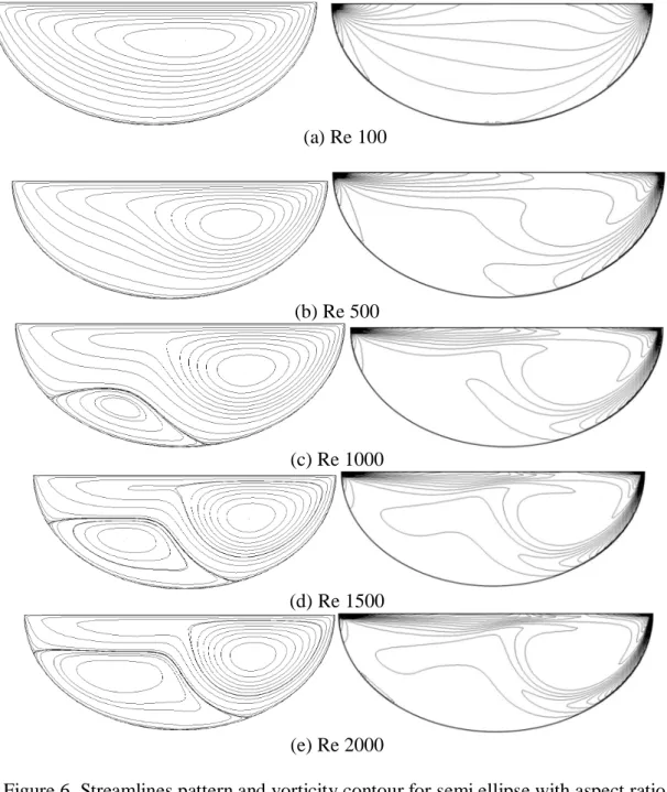
Meanwhile, for aspect ratio 3/8, the streamlines pattern and vorticity contour are presented in Figure 6. It can be observed that there are no secondary vortex developed inside the cavity at Reynolds number 100 and 500. Secondary vortex only appeared when Reynolds number increases from 1000 until 2000. Regarding the value of stream function, the magnitudes increase from 0.05376 to 0.05888 when the Reynolds number increases from 100 to 500. Even so, the magnitudes of the stream function decrease from 0.05874 to 0.05538 when the Reynolds number increases from 1000 to 2000. This phenomenon is mostly due to the occurrence of secondary vortex rotation which counter rotates the primary vortex rotating direction. Therefore, the secondary vortex acts as an obstacle to the primary vortex, thus reducing the value of the peak streamfunction even though the Reynolds number is rising. For the vorticity contour, the significant changes can be observed at the right sight of the cavity where the centre of primary vortex is located. The stream function peak value and its location for both secondary and primary vortex are provided in Table 5.
213 (a) Re 100 (b) Re 500 (c) Re 1000 (d) Re 1500 (e) Re 2000
Figure 6. Streamlines pattern and vorticity contour for semi ellipse with aspect ratio, AR of 3/8 for Re 100, 500, 1000, 1500 and 2000.
Table 5. The primary and secondary vortex centre location and streamfunction values for aspect ratio of 3/8 with various Reynolds number.
Re Primary vortex centre location Streamfunction value, Secondary vortex centre location Streamfunction value, 100 (0.5975, 0.1176) 0.05376 - - 500 (0.6913, 0.1350) 0.05888 - - 1000 (0.6913, 0.1435) 0.05874 (0.3201, 0.2518) 0.00126 1500 (0.7138, 0.1435) 0.05716 (0.3087, 0.2083) 0.00379 2000 (0.7357, 0.1350) 0.05538 (0.2862, 0.1928) 0.00505
214
The angle of separation and reattachment of the secondary vortex for aspect ratio 3/8 or 3/4 of half ellipse are presented in Table 6. Similar for aspect ratio 3/4, the secondary vortex starts to appear inside the cavity at Re number 1000. Initially, the primary vortex separates from the boundary at the angle of 30.341º and then reattached to the curvilinear boundary when the angle reach 103.264º. The primary vortex separates earlier at the angle of 19.531º and reattached at later angle of 115.505º for Reynolds number of 1500. While, the primary vortex separate at half separation angle is 15.022º for Reynolds number of 2000. Meanwhile, for the reattachment angle, the value is 123.867º which is greater than for Reynolds number 1500. The differences between the separation angle and reattachment angle increases as the Reynolds number increases.
Table 6. Angles of separation and reattachment of secondary vortex (in degree).
Re
1000 30.341 103.264
1500 19.531 115.505
2000 15.022 123.867
CONCLUSIONS
The lid driven cavity flow inside shallow semi-ellipse lid driven cavity was simulated for different aspect ratios and Reynolds number. The primary and secondary vortex behaviour was observed together with the vortex centre location and peak stream function magnitude value. The angle of separation and reattachment for primary and secondary vortex were obtained when the secondary vortex value developed. It can be seen that as Reynolds number increase to an average of 1000 for every aspect ratios, secondary vortex developed in the cavity. As the Reynolds number increase, the size of secondary vortex also increase. The increment depth of the cavity also played an important element in the relationship between Reynolds number and secondary vortex. Non uniform finite difference method has been demonstrated to be successful for simulating non-square finite different problem.
ACKNOWLEDGMENTS
The authors would like to thank Universiti Malaysia Pahang for provides laboratory facilities and financial support under project no. RDU110382.
REFERENCES
Albensoeder, S., Kuhlmann, H.C. and Rath, H.J. 2001. Multiplicity of steady two-dimensional flows in two-sided lid-driven cavities. Theoretical and Computational Fluid Dynamics, 14: 223-241.
Azwadi, C.S.N. and Idris, M.S. 2010. Finite different and lattice boltzmann modelling for simulation of natural convection in a square cavity. International Journal of Mechanical and Materials Engineering, 5: 80-86.
Barragy, E. and Carey, G.F. 1997. Stream function-vorticity driven cavity solution using P finite elements. Computers and Fluids, 26: 453-468.
215
Botella, O. 1997. On The solution of the Navier-stokes equations using Chebyshev projection schemes with third-order accuracy in time. Computers and Fluids, 26: 107-116.
Botella, O. and Peyret, R. 1998. Benchmark spectral results on the lid-driven cavity flow. Computers and Fluids, 27: 421-433.
Chang, M.H. and Cheng, C.H. 1999. Predictions of lid-driven flow and heat convection in an arc-shape cavity. International Communications in Heat and Mass Transfer, 26: 829-838.
Cheng, C.H. and Chen, C.L. 2005. Buoyancy-induced periodic flow and heat transfer in lid-driven cavities with different cross-sectional shapes. International Communications in Heat and Mass Transfer, 32: 483-490.
Cheng, M. and Hung, K.C. 2006. Vortex structure of steady flow in a rectangular cavity. Computers and Fluids, 35: 1046-1062.
Erturk, E. and Gokcol, O. 2007. Fine grid numerical solutions of triangular cavity flow. Epj Applied Physics, 38: 97-105.
Ghia, U., Ghia, K.N. and Shin, C.T. 1982. High-Re Solutions for incompressible flow using the Navier-stokes equations and a multigrid method. Journal of Computational Physics, 48: 387-411.
Jyotsna, R. and Vanka, S.P. 1995. Multigrid calculation of steady, viscous flow in a triangular cavity. Journal of Computational Physics, 122: 107-117.
Koseff, J.R. and Street, R.L. 1984a. On end wall effects in a lid-driven cavity flow. Journal of Fluids Engineering, Transactions of The ASME, 106: 385-389.
Koseff, J. R. and Street, R.L. 1984b. Visualization studies of a shear driven three-dimensional recirculating flow. Journal of Fluids Engineering, Transactions of The ASME, 106: 21-29.
Kosinski, P., Kosinska, A. and Hoffmann, A.C. 2009. Simulation of solid particles behaviour in a driven cavity flow. Powder Technology, 191: 327-339.
Li, M. and Tang, T. 1996. Steady viscous flow in a triangular cavity by efficient numerical techniques. Computers and Mathematics with Applications, 31: 55-65.
McQuain, W.D., Ribbens, C.J., Wang, C.Y. and Watson, L.T. 1994. Steady viscous flow in a trapezoidal cavity. Computers and Fluids, 23: 613-626.
Mercan, H. and Atalik, K. 2009. Vortex Formation in lid-driven arc-shape cavity flows at high reynolds numbers. European Journal of Mechanics, B/Fluids, 28: 61-71. Peri , M., Kessler, R. and Scheuerer, G. 1988. Comparison of finite-volume numerical
methods with staggered and colocated grids. Computers and Fluids, 16: 389-403.
Prasad, A.K. and Koseff, J.R. 1989. Reynolds number and end-wall effects on a lid-driven cavity flow. Physics of Fluids A, 1: 208-218.
Ribbens, C.J. 1994. Steady viscous flow in a triangular cavity. Journal of Computational Physics, 112: 173-181.
Veldman, A.E.P. and Rinzema, K. 1992. Playing with nonuniform grids. Journal of Engineering Mathematics, 26: 119-130.
Wahba, E.M. 2009. Multiplicity of states for two-sided and four-sided lid driven cavity flows. Computers and Fluids, 38: 247-253.
Weinan, E. and Liu, J.G. 1996. Vorticity boundary condition and related issues for finite difference schemes. Journal of Computational Physics, 124: 368-382.
Zdanski, P.S.B., Ortega, M.A. and Fico Jr, N.G.C.R. 2003. Numerical study of the flow over shallow cavities. Computers and Fluids, 32: 953-974.
216
Zhang, T., Shi, B. and Chai, Z. 2010. Lattice Boltzmann simulation of lid-driven flow in trapezoidal cavities. Computers and Fluids, 39: 1977-1989.
Zin, M.R.M. and Sidik, N.A.C. 2010. An accurate numerical method to predict fluid flow in a shear driven cavity. International Review of Mechanical Engineering, 4: 719-725.