Distributed Computation and Optimization over Networks

(1)

UNIVERSITY OF OKLAHOMA GRADUATE COLLEGE

DISTRIBUTED COMPUTATION AND OPTIMIZATION OVER NETWORKS

A DISSERTATION

SUBMITTED TO THE GRADUATE FACULTY in partial fulfillment of the requirements for the

Degree of DOCTOR OF PHILOSOPHY By JIE LU Norman, Oklahoma 2011

(2)

A DISSERTATION APPROVED FOR THE

SCHOOL OF ELECTRICAL AND COMPUTER ENGINEERING

BY

Dr. Choon Yik Tang, Chair

Dr. Nikola Petrov

Dr. J.R. Cruz

Dr. Joseph P. Havlicek

(3)

c

(4)

(5)

Acknowledgements

I would like to express deep gratitude to my advisor, Dr. Choon Yik Tang, for providing tremendous mentoring, help, and support throughout my Ph.D. program. I want to thank him for leading me into the world of research and consistently providing invaluable guidance in every stage of my research.

I am grateful to Dr. J.R. Cruz, Dr. Joseph P. Havlicek, Dr. Nikola Petrov, and Dr. Thordur Runolfsson for their interests in my research and for serving on my dissertation committee. I have greatly benefited from their insightful suggestions on my work.

I also wish to thank my parents, Zhiping Lu and Peifang Zhang, for their endless love, care, and support. Special thanks to my mother who came to Norman and stayed with me for the last six months.

Finally, financial support from the National Science Foundation is grate-fully acknowledged.

(6)

Appendix B. Proofs for Chapter 3 195 B.1 Proof of Lemma 3.1 . . . 195 B.2 Proof of Proposition 3.1 . . . 196 B.3 Proof of Theorem 3.1 . . . 196 B.4 Proof of Corollary 3.1 . . . 197 B.5 Proof of Lemma 3.2 . . . 197 B.6 Proof of Theorem 3.2 . . . 202 B.7 Proof of Corollary 3.2 . . . 202 B.8 Proof of Theorem 3.3 . . . 203 B.9 Proof of Corollary 3.3 . . . 203

(9)

Appendix C. Proofs for Chapter 4 204 C.1 Proof of Theorem 4.1 . . . 204 C.2 Proof of Theorem 4.2 . . . 205 C.3 Proof of Theorem 4.3 . . . 205 C.4 Proof of Theorem 4.4 . . . 205 C.5 Proof of Theorem 4.5 . . . 206 C.6 Proof of Theorem 4.6 . . . 209

Appendix D. Proofs for Chapter 5 210 D.1 Proof of Theorem 5.1 . . . 210

D.2 Proof of Theorem 5.2 . . . 213

D.3 Proof of Theorem 5.3 . . . 214

Appendix E. Proofs for Chapter 6 215 E.1 Proof of Theorem 6.1 . . . 215

(10)

List of Tables

(11)

List of Figures

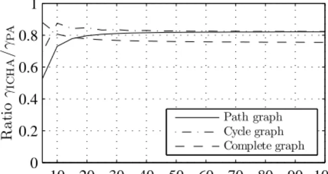
2.1 Comparison between the stochastic convergence rate 1− 1 γPA of

PA and the deterministic bound 1₋ 1

γICHA on convergence rate

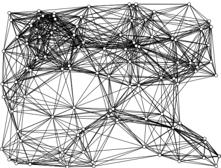
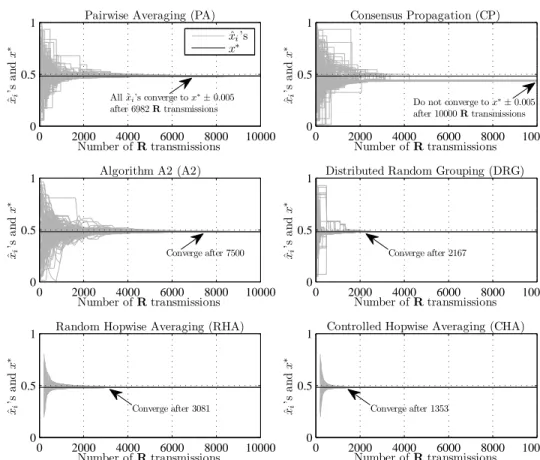
of ICHA for path, cycle, and complete graphs. . . 37 2.2 A 100-node, 1000-link multi-hop wireless network. . . 46 2.3 Convergence of the estimates ˆxi(k)’s to the unknown average x∗

under PA, CP, A2, DRG, RHA, and CHA for the network in Figure 2.2. . . 47 2.4 Bandwidth/energy efficiency of flooding, PA, CP, A2, DRG,

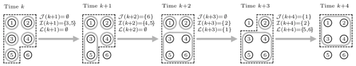
RHA, and CHA on random geometric networks with varying number of nodes N and average number of neighbors 2L_N. . . 50 3.1 An example showing that an agent network is connected at time

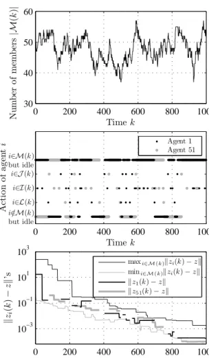
k. . . 64 3.2 Simulation result illustrating the use of SE to perform

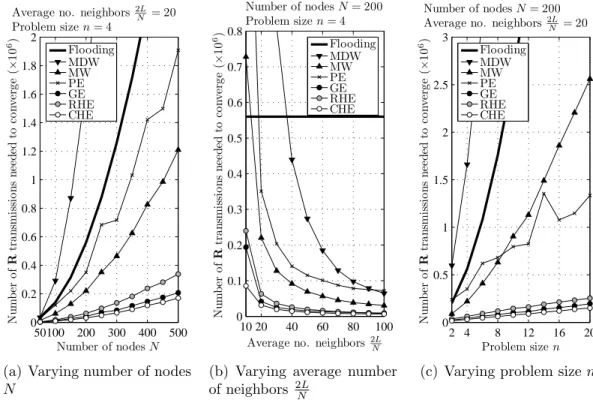
uncon-strained quadratic optimization over a volatile multi-agent system. 73 4.1 Performance comparison on multi-hop wireless networks with

varying number of nodesN, varying average number of neighbors

2L

N, and varying problem size n. . . 95

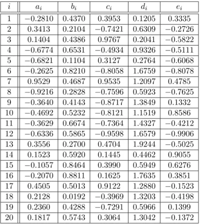
5.1 A 20-node, 30-link network with each nodeiobserving a function fi. . . 118

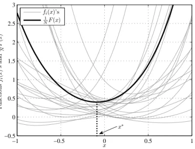
5.2 Graphs of the functions fi’s and _N1F, along with the unknown

optimizer x∗_{. . . 119}

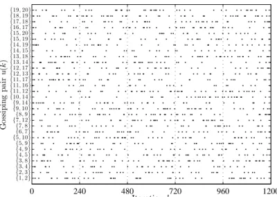
5.3 A realization of the random sequence (u(k))1200

k=1 of gossiping pairs.120

5.4 Convergence of the valueV(x(k)) of the common Lyapunov func-tion to zero. . . 121 5.5 Convergence of the estimates ˆxi(k)’s to the unknown optimizer

x∗. . . 121 6.1 Performance comparison on random geometric wireless networks

with varying number of nodes N and average number of neigh-bors 2L_N. . . 151

(12)

Abstract

Jie Lu, Ph.D.

The University of Oklahoma, 2011 Supervisor: Choon Yik Tang

This dissertation is devoted to the development of efficient, robust, and scal-able distributed algorithms, which enscal-able agents in a large-scale, multi-hop network to cooperatively compute a global quantity, or solve an optimization problem, with only local interactions and without any centralized coordination. Algorithms of this nature are attracting growing interest from a number of sci-entific communities due to their broad application, for example, to autonomous agent coordination and control in mobile ad hoc networks, distributed signal processing and data fusion in wireless sensor networks, and studies of opinion dynamics in social networks.

In this dissertation, we address three fundamental problems in the area, namely: averaging, solving of positive definite linear equations, and uncon-strained separable convex optimization. Based on a blend of tools and ideas from system, optimization, and graph theories, we construct a novel set of distributed algorithms—including continuous- and discrete-time, gossip and asynchronous—which solve these problems over undirected networks with ar-bitrary (and, in some cases, time-varying) topologies and agent memberships. We also analyze the properties of these algorithms, including their convergence

(13)

rates and complexity characteristics, and compare them with existing schemes, showing analytically and numerically that our algorithms possess several ap-pealing features.

The major contributions of this dissertation are as follows: first, we show that Lyapunov stability theory may be used to shape the behavior of asynchronous distributed algorithms. This finding allows us to introduce the notion of greedy, decentralized, feedback iteration control, leading to a class ofControlled Hopwisealgorithms, which are highly bandwidth/energy efficient in wireless networks. The finding also creates a new paradigm in the design of asynchronous distributed algorithms, where iterations are opportunistically controlled, as opposed to being randomized.

Second, we show that the Bregman divergence of the Lagrangian of a separable convex optimization problem may be used to form a common Lya-punov function. This result enables us to derive a family ofZero-Gradient-Sum algorithms, which yield nonlinear networked dynamical systems on an invariant manifold, and which differ fundamentally from, and have pros and cons over, the existing subgradient algorithms. The derivation also shows that a gossip variant within the family generalizes the classic Pairwise Averaging, and the family itself is a natural generalization of several well-known algorithms for distributed consensus, to distributed convex optimization.

Finally, we provide a series of analysis of the properties of our algorithms (e.g., boundedness, asymptotic and exponential convergence, lower and upper bounds on convergence rates, scalability) on various networks (e.g., path, cycle, regular, complete, and general graphs), describing explicitly the dependency of such properties on network topologies, problem characteristics, and algorithm

(14)

parameters, including the algebraic connectivity, Laplacian spectral radius, and function curvatures.

(15)

Chapter 1 Introduction

1.1 Motivation

Emerging technologies on intelligent devices have triggered the vision of many applications of large-scale networks, including target tracking by a mobile ad hoc network [15, 71], estimation of a physical phenomenon by a wireless sensor network [1,18], demonstration of flocking/swarming by a team of mobile robots [7, 49], resource allocation in a computer network [14, 29], and study of social interactions and opinion dynamics in a social network [12,33]. To realize these applications, nodes in such networks may have to operate autonomously in dynamic and infrastructure-less environments with severe bandwidth and energy constraints, communicate in multi-hop fashion over unreliable links, and accomplish tasks that require extensive processing of information, rapid decentralized decision making, and precise coordination of actions. Therefore, it is highly desirable that such networks possess the ability to perform in-network computation and optimization: efficiently compute a quantity or solve an optimization problem, where the data that determine the quantity or the problem are distributed across network and observed by nodes.

In principle, in-network computation and optimization may be accom-plished via flooding, whereby every node floods the network with its observa-tion, as well as acentralizedscheme, whereby a central node uses an overlay tree to collect all the node observations, calculate the solution, and send it back to

(16)

every node. These two methods, unfortunately, have serious limitations: flood-ing is extremely bandwidth and energy inefficient because it propagates redun-dant information across the network, ignoring the fact that the ultimate goal is to simply determine the desirable quantity or an optimizer. The centralized scheme, on the other hand, is vulnerable to node mobility, node membership changes, and single-point failures, making it necessary to frequently maintain the overlay tree and occasionally start over with a new central node, both of which are rather costly to implement.

The limitations of flooding as well as the centralized scheme have mo-tivated the search for distributed algorithms where each node in a network communicates and shares information with its neighbors only. Clearly, such algorithms require neither flooding of node observations, nor construction of overlay trees and routing tables, to execute. Moreover, the decentralized nature of distributed algorithms makes them more robust to dynamic environments and unreliable links. Thus, the goal of this research is to develop robust, scal-able, and efficient distributed algorithms for computation and optimization over networks.

1.2 Literature Review

The current literature provides a growing collection of distributed al-gorithms for in-network computation and optimization, which may be simply referred to as distributed computationand distributed optimization.

For distributed computation, one line of research is distributed aver-aging, i.e., computing the network-wide average of node observations. This problem arises in many applications. For example, by averaging their

(17)

indi-vidual throughputs, an ad hoc network of computers can assess how well the network, as a whole, is performing, and by averaging their humidity mea-surements, a wireless network of sensing agents can cooperatively detect the occurrence of local, deviation-from-average anomalies. To date, a collection of distributed averaging schemes with continuous-time [16, 52, 69], discrete-time synchronous [20, 30, 31, 52, 53, 55, 56, 64, 69, 74, 75, 78], and discrete-time asyn-chronous [8, 11, 13, 20, 26, 36, 38, 39, 72] settings have been developed.

Another distributed computation problem is to determine the solution for a system of linear equations where each parameter is the sum of a set of node observations. Examples of its applications include finding the least-squares solution of a distributed sensor fusion problem [76, 77] and solving unconstrained quadratic programming problems over networks. The current literature offers several distributed algorithms for solving this problem, includ-ing the continuous-time algorithm in [66], as well as the discrete-time algorithms in [76, 77] which find the solution by computing the average of each parameter of the linear equations.

In addition, distributed algorithms for finding the maximum of node observations have been introduced in [13, 17, 39, 41, 68]. In [26, 30, 39, 41], the problem of decentralizedly computing the sum of node observations has been explored. Distributed algorithms for computing the power mean of node ob-servations have also been reported in [2, 17, 39]. Furthermore, distributed con-sensus, a topic closely related to distributed computation, where nodes seek to achieve an arbitrary network-wide consensus on their individual opinions, has also been extensively studied; see [4, 34] for early treatments, [20, 21, 24, 25, 40, 52, 54, 63, 67, 70] for more recent work, and [50] for a survey.

(18)

Distributed optimization problems are generally more complicated com-pared to distributed computation, among which the most common problem may bedistributed convex optimization, where the objective and constraint functions are all convex. A special case of distributed convex optimization is that the objective function is the sum of the convex functions observed by nodes, which has found diverse applications. For example, least-squares estimation [65], ro-bust estimation [65], energy-based source localization [57], and clustering and density estimation [57] are all in the form of this special case. As another example, consider a social network, where each individual’s level of dissatisfac-tion if the network takes a decision may be represented by a convex funcdissatisfac-tion, so that finding an optimal decision means minimizing the total dissatisfac-tion across the network, where everyone’s voice is heard. To date, a family of discrete-time subgradient algorithms [27,28,32,42–47,57–62,65] for solving this problem have been reported in the literature. These algorithms may be clas-sified into two groups. The first group is incremental [28, 42–44, 57–59, 61, 65], relying on the passing of an estimate on an optimizer of the convex optimiza-tion problem. Incremental subgradient algorithms can be further categorized into cyclic ones [42–44, 57–59, 61, 65], which require the estimate to be passed along a Hamiltonian cycle that visits every node exactly once, and non-cyclic ones [28,42–44], which allow the estimate to be passed around the network ran-domly. The second group is non-incremental [27, 32, 45–47, 60, 62], which relies instead on combining subgradient updates with linear consensus iterations. All these subgradient algorithms need appropriate choices of stepsizes to let the estimate(s) move along the gradient of the observed functions and approach an optimizer of the problem.

(19)

1.3 Original Contributions

In this dissertation, a collection of distributed algorithms that solve three fundamental in-network computation and optimization problems, namely, averaging, solving of positive definite linear equations, and unconstrained sep-arable convex optimization, are designed and analyzed.

The dissertation starts with addressing the problem of averaging num-bers across a wireless network from an important, but largely neglected, view-point: bandwidth/energy efficiency. We show that existing distributed averag-ing schemes have several drawbacks and are inefficient, producaverag-ing networked dynamical systems that evolve with wasteful communications. Motivated by this, we develop Controlled Hopwise Averaging (CHA), a distributed asyn-chronous algorithm that attempts to “make the most” out of each iteration by fully exploiting the broadcast nature of wireless medium and enabling control of when to initiate an iteration. We show that CHA admits a common quadratic Lyapunov function for analysis, derive bounds on its exponential convergence rate, and show that they outperform the convergence rate of Pairwise Averag-ing for some common graphs. We also introduce a new way to apply Lyapunov stability theory, using the Lyapunov function to perform greedy, decentralized, feedback iteration control. Through extensive simulation on random geometric graphs, we show that CHA is substantially more efficient than several existing schemes, requiring far fewer transmissions to complete an averaging task.

Next, a family of distributed asynchronous algorithms for solving sym-metric positive definite systems of linear equations over agent and wireless networks are constructed. In particular, we develop Subset Equalizing (SE), a Lyapunov-based algorithm for solving the problem over agent networks with

(20)

arbitrary asynchronous interactions and spontaneous membership dynamics, both of which may be exogenously driven and completely unpredictable. To analyze the behavior of SE, we introduce several notions of network connec-tivity, capable of handling such interactions and membership dynamics, and a time-varying quadratic Lyapunov-like function, defined on a state space with changing dimension. Based on them, we derive sufficient conditions for ensur-ing the boundedness, asymptotic convergence, and exponential convergence of SE, and show that these conditions are mild. Moreover, we study the inter-play among wireless communications, distributed algorithms, and control in solving such quadratic optimization problems over multi-hop wireless networks with fixed topologies. Building on the results from SE, we develop and analyze Pairwise, Groupwise, Random Hopwise, and Controlled Hopwise Equalizing (PE, GE, RHE, and CHE), showing along the way how the broadcast nature of wireless transmissions may be fully utilized, how undesirable overlapping iterations may be avoided, and how iterations may be feedback controlled in a greedy, decentralized, Lyapunov-based fashion, leading to CHE, which yields provable exponential convergence and a quantifiable bound on the convergence rate. Through extensive simulation, we show that GE, RHE, and CHE are dramatically more efficient and scalable than two existing, average-consensus-based schemes, with CHE having the best performance.

Finally, we address the problem of distributed convex optimization from both discrete- and continuous-time standpoints. More specifically, with a few additional mild assumptions, we develop two gossip-style, non-gradient-based algorithms, referred to as Pairwise Equalizing(PE) and Pairwise Bisectioning (PB), for achieving unconstrained, separable, convex optimization over undi-rected networks with time-varying topologies, which are fundamentally

(21)

differ-ent from the existing subgradidiffer-ent algorithms. We show that PE and PB are easy to implement, bypass limitations of the subgradient algorithms, and pro-duce switched, nonlinear, networked dynamical systems that admit a common Lyapunov function based on the Bregman divergence [10] and asymptotically converge. Moreover, PE generalizes the well-known Pairwise Averaging and Randomized Gossip Algorithm and extends naturally to networks with both time-varying topologies and node memberships, while PB relaxes a require-ment of PE, allowing nodes to never share their local functions. Furthermore, we introduce a new approach to the problem: control of distributed convex op-timization, which extends the ideas of PE and the notion of greedy, decentral-ized, feedback iteration control for CHA using the Bregman-divergence-based Lyapunov function for PE and PB. The resulting distributed asynchronous al-gorithm, referred to as Controlled Hopwise Equalizing(CHE), is shown via ex-tensive simulation to be significantly more bandwidth/energy efficient than sev-eral existing subgradient algorithms over wireless networks with fixed topolo-gies, requiring far less communications to solve a convex optimization problem. In addition to the above discrete-time distributed algorithms, we derive a set of continuous-time distributed algorithms that solve the problem over undi-rected networks with fixed topologies. The algorithms are developed using a Lyapunov function candidate that exploits convexity, and are called Zero-Gradient-Sum (ZGS) algorithms as they yield nonlinear networked dynamical systems that evolve invariantly on a zero-gradient-sum manifold and converge asymptotically to the unknown optimizer. We also describe a systematic way to construct ZGS algorithms, show that a subset of them actually converge exponentially, and obtain lower and upper bounds on their convergence rates in terms of the network topologies, problem characteristics, and algorithm

(22)

pa-rameters, including the algebraic connectivity, Laplacian spectral radius, and function curvatures. The findings may be regarded as a natural generaliza-tion of several well-known algorithms and results for distributed consensus, to distributed convex optimization.

1.4 Dissertation Outline

The outline of this dissertation is as follows: Chapter 2 studies dis-tributed averaging over networks, in which CHA is developed. Chapters 3–4 present distributed algorithms for solving positive definite linear equations over networks. In particular, Chapter 3 proposes SE for agent networks and Chap-ter 4 constructs a few distributed algorithms for wireless networks. ChapChap-ters 5– 7 address the problem of distributed convex optimization over networks, where PE and PB are developed in Chapter 5, CHE is introduced in Chapter 6, and ZGS algorithms are constructed in Chapter 7. Finally, Chapter 8 concludes the dissertation and provides several possible future research directions. The proofs for Chapters 2–6 are included in Appendices A–E, respectively.

(23)

Chapter 2 Controlled Hopwise Averaging

2.1 Introduction

Distributed averaging is a fundamental problem in distributed compu-tation that finds many applications in multi-agent systems, ad hoc networks, sensor networks and the likes. Due to its significance, the problem has been widely studied (see, e.g., [8, 11, 13, 16, 20, 26, 30, 31, 36, 38, 39, 52, 53, 55, 56, 64, 69, 72, 74, 75, 78]) for different network models (e.g., wired or wireless; undirected or directed links; fixed or time-varying topologies), with different communica-tion assumpcommunica-tions (e.g., without delays, errors, and quantizacommunica-tion or with), and in different time domains (e.g., continuous- or discrete-time; synchronous or asynchronous). The research efforts have led to a growing list of algorithms, including Pairwise Averaging [72], Randomized Gossip Algorithm [8], Accel-erated Gossip Algorithm [11], Distributed Random Grouping [13], and Linear Prediction-Based Accelerated Averaging [56], to name just a few.

Although the current literature offers a rich collection of distributed av-eraging schemes along with in-depth analysis of their behaviors, their efficacy from a bandwidth/energy efficiency standpoint has not been examined. This chapter is devoted to studying the distributed averaging problem from this standpoint. Its contributions are as follows: we first show that the existing schemes—regardless of whether they are developed in continuous- or discrete-time, for synchronous or asynchronous models—have a few deficiencies and are

(24)

inefficient, producing networked dynamical systems that evolve with wasteful communications. To address these issues, we develop Random Hopwise Av-eraging (RHA), an asynchronous distributed averaging algorithm with several positive features, including a novel one among the asynchronous schemes: an ability to fully exploit the broadcast nature of wireless medium, so that no overheard information is ever wastefully discarded. We show that RHA ad-mits a common quadratic Lyapunov function, is almost surely asymptotically convergent, and eliminates all but one of the deficiencies facing the existing schemes.

To tackle the remaining deficiency, on lack of control, we introduce the concept of feedback iteration control, whereby individual nodes use feedback to control when to initiate an iteration. Although simple and intuitive, this concept, somewhat surprisingly, has not been explored in the literature on dis-tributed averaging [8, 11, 13, 16, 20, 26, 30, 31, 36, 38, 39, 52, 53, 55, 56, 64, 69, 72, 74, 75, 78] and distributed consensus [4, 20, 21, 24, 25, 34, 40, 50, 52, 54, 63, 67, 70]. We show that RHA, along with the common quadratic Lyapunov function, exhibits features that enable a greedy, decentralized approach to feedback iter-ation control, which leads to bandwidth/energy-efficient iteriter-ations at zero feed-back cost. Based on this approach, we present two modified versions of RHA: an ideal version referred to asIdeal Controlled Hopwise Averaging(ICHA), and a practical one referred to simply asControlled Hopwise Averaging(CHA). We show that ICHA yields a networked dynamical system with state-dependent switching, derive deterministic bounds on its exponential convergence rate for general and specific graphs, and show that the bounds are better than the stochastic convergence rate of Pairwise Averaging [20, 72] for path, cycle, and complete graphs. We also show that CHA is able to closely mimic the

(25)

be-havior of ICHA, achieving the same bounds on its convergence rate. Finally, via extensive simulation on random geometric graphs, we demonstrate that CHA is substantially more bandwidth/energy efficient than Pairwise Averag-ing [72], Consensus Propagation [38], Algorithm A2 of [36], and Distributed Random Grouping [13], requiring far fewer transmissions to complete an aver-aging task. In particular, CHA is twice more efficient than the most efficient existing scheme when the network is sparsely connected.

The outline of this chapter is as follows: Section 2.2 formulates the distributed averaging problem. Section 2.3 describes the deficiencies of the existing schemes. Sections 2.4 and 2.5 develop RHA and CHA and characterize their convergence properties. In Section 2.6, their comparison with several existing schemes is carried out. Finally, Section 2.7 concludes the chapter. The proofs of the main results are included in Appendix A.

2.2 Problem Formulation

Consider a multi-hop wireless network consisting of N _≥ 2 nodes, con-nected by Lbidirectional links in a fixed topology. The network is modeled as a connected, undirected graph G = (V,E), whereV ={1,2, . . . , N} represents the set of N nodes (vertices) and E ⊂ {{i, j} : i, j ∈ V, i 6= j} represents the set of L links (edges). Any two nodes i, j ∈ V are one-hop neighbors and can communicate if and only if _{i, j_{} ∈ E}. The set of one-hop neighbors of each node i _{∈ V} is denoted as _Ni = {j ∈ V : {i, j} ∈ E}, and the

communica-tions are assumed to be delay- and error-free, with no quantization. Each node i _{∈ V} observes a scalar yi ∈ R, and all the N nodes wish to determine the

(26)

network-wide average x∗ _∈_R _{of their individual observations, given by} x∗ = 1 N X i∈V yi. (2.1)

Given the above model, the problem addressed in this chapter is how to construct a distributed averaging algorithm—continuous- or discrete-time, synchronous or otherwise—with which each node i ∈ V repeatedly communi-cates with its one-hop neighbors, iteratively updates its estimate ˆxi ∈ R of

the unknown averagex∗ _{in (2.1), and asymptotically drives ˆ}_x

i tox∗—all while

consuming bandwidth and energy efficiently.

The bandwidth/energy efficiency of an algorithm is measured by the number of real-number transmissions it needs to drive all the xˆi’s to a

suf-ficiently small neighborhood of x∗_{, essentially completing the averaging task.}

This quantity is a natural measure of efficiency because the smaller it is, the lesser bandwidth is occupied, the lesser energy is expended for communica-tions, and the faster an averaging task may be completed. These, in turn, imply more bandwidth and time for other tasks, smaller probability of colli-sion, longer lifetime for battery-powered nodes, and possible earlier return to sleep mode, all of which are desirable. The quantity also allows algorithms with different numbers of real-number transmissions per iteration to be fairly com-pared. Although, in networking, every message inevitably contains overhead (e.g., transmitter/receiver IDs and message type), we exclude such overhead when measuring efficiency since it is not inherent to an algorithm, may be re-duced by piggybacking messages, and becomes negligible when averaging long vectors.

(27)

2.3 Deficiencies of Existing Schemes

As was pointed out in Section 2.1, the current literature offers a va-riety of distributed averaging schemes for solving the problem formulated in Section 2.2. Unfortunately, as is explained below, they suffer from a number of deficiencies, especially a lack of bandwidth/energy efficiency, by producing networked dynamical systems that evolve with wasteful real-number transmis-sions.

The continuous-time algorithms in [16, 52, 69] have the following defi-ciency:

D1. Costly discretization: As immensely inefficient as flooding is, the continuous-time algorithms in [16, 52, 69] may be more so: flooding only requiresN2

real-number transmissions for all the N nodes to exactly determine the average x∗ _{(since it takes} _N _{real-number transmissions for each node}

i ∈ V to flood the network with its yi), whereas these algorithms may

need far more than that to essentially complete an averaging task. For instance, the algorithm in [52] updates the estimates ˆxi’s of x∗ according

to the differential equation dˆxi(t)

dt = X

j∈Ni

(ˆxj(t)−xˆi(t)), ∀i∈ V. (2.2)

To realize (2.2), each node i _{∈ V} has to continuously monitor the ˆxj(t)

of every one-hop neighbor j _{∈ N}i. If this can be done without wireless

communications (e.g., by direct sensing), then the bandwidth/energy effi-ciency issue is moot. If wireless communications must be employed, then (2.2) has to be discretized, either exactly via a zero-order hold, i.e.,

ˆ

xi((k+ 1)T) =

X

j∈V

(28)

or approximately via numerical techniques such as the Euler forward difference method, i.e.,

ˆ xi((k+ 1)T)−xˆi(kT) T = X j∈Ni (ˆxj(kT)−xˆi(kT)), ∀i∈ V, (2.4)

where each hij ∈ R is the ij-entry of e−LT, L ∈ RN×N is the Laplacian

matrix of the graph _G that governs the dynamics (2.2), and T > 0 is the sampling period. Regardless of (2.3) or (2.4), they may be far more costly to realize than flooding: with (2.3),N2 _{real-number transmissions}

are already needed per iteration (since, in general, hij 6= 0 ∀i, j ∈ V, so

that each node i∈ V has to flood the network with its ˆxi(kT), for every

k). In contrast, with (2.4), onlyN real-number transmissions are needed per iteration (since each node i ∈ V only has to wirelessly transmit its ˆ

xi(kT) once, to every one-hop neighbor j ∈ Ni, for every k). However,

the number of iterations, needed for all the ˆxi(kT)’s to converge to an

acceptable neighborhood of x∗_{, may be very large, since the sampling}

period T must be sufficiently small for (2.4) to be stable. If the number of iterations needed exceeds N—which is possible and likely so with a conservatively small T—then (2.4) would be worse than flooding1_.

The discrete-time synchronousalgorithms in [20, 30, 31, 52, 53, 55, 56, 64, 69, 74, 75, 78] have the following deficiencies:

D2. Clock synchronization: The discrete-time synchronous algorithms in [20, 30,31,52,53,55,56,64,69,74,75,78] require all theN nodes to always have the same clock to operate. Although techniques for reducing clock syn-1_{Flooding is, of course, more storage and bookkeeping intensive.}

(29)

chronization errors are available, it is still desirable that this requirement can be removed.

D3. Forced transmissions: The algorithms in [20,31,52,53,55,56,64,69,74,75] update the estimates ˆxi’s of x∗ according to the difference equation

ˆ

xi(k+ 1) =wii(k)ˆxi(k) +

X

j∈Ni

wij(k)ˆxj(k), ∀i∈ V, (2.5)

where each wij(k) ∈ R is a weighting factor that is typically constant.

The wij(k)’s may be specified in several ways, including choosing them

to maximize the convergence rate [74] or minimize the mean-square de-viation [75]. However, no matter how thewij(k)’s are chosen, these

algo-rithms are bandwidth/energy inefficient because the underlying update rule (2.5) simply forces every node i∈ V at each iterationk to transmit its ˆxi(k) to its one-hop neighbors, irrespective of whether such

transmis-sions are worthy. It is possible, for example, that the ˆxi(k)’s of a cluster

of nearby nodes are almost equal, so that their ˆxi(k+ 1)’s, being convex

combinations of their ˆxi(k)’s, are also almost equal, causing their

trans-missions to be unworthy. The fact that N real-number transmissions are needed per iteration also implies that (2.5) must drive all the ˆxi(k)’s to

an acceptable neighborhood of x∗ within at most N iterations, in order to just outperform flooding.

D4. Computing intermediate quantities: The scheme in [53] uses two parallel runs of a consensus algorithm to obtain two consensus values and defines each ˆxi(k) as the ratio of these two values. While possible, this scheme is

likely inefficient because it attempts to compute two intermediate quan-tities, as opposed to computing x∗ directly.

(30)

72] have the following deficiencies:

D5. Wasted receptions: Each iteration of Pairwise Averaging [72], Anti-Entropy Aggregation [26, 39], Randomized Gossip Algorithm [8], and Accelerated Gossip Algorithm [11] involves a pair of nodes transmitting to each other their state variables. Due to the broadcast nature of wireless medium, their transmissions are overheard by unintended nearby nodes, who would immediately discard this “free” information, instead of using it to possi-bly speed up convergence, enhancing bandwidth/energy efficiency. Hence, these algorithms result in wasted receptions. The same can be said about Consensus Propagation [38] and Algorithm A2 of [36], although they do not assume pairwise exchanges. It can also be said about Distributed Random Grouping [13], which only slightly exploits such broadcast na-ture: the leader of a group does, but the members, who contribute the majority of the transmissions, do not.

D6. Overlapping iterations: Pairwise Averaging [72], Anti-Entropy Aggrega-tion [26, 39], Randomized Gossip Algorithm [8], Accelerated Gossip Al-gorithm [11], and Distributed Random Grouping [13] require sequential transmissions from multiple nodes to execute an iteration. This suggests that before an iteration completes, the nodes involved may be asked to participate in other iterations initiated by those unaware of the ongo-ing iteration. Thus, these algorithms are prone to overlappongo-ing iterations and, therefore, to deadlock situations [36]. It is noted that this practical issue is naturally avoided by Consensus Propagation [38] and explicitly handled by Algorithms A1 and A2 of [36].

D7. Uncontrolled iterations: The discrete-time asynchronous algorithms in [8, 11, 13, 26, 36, 38, 39, 72] do not let individual nodes use information

(31)

available to them during runtime (e.g., history of the state variables they locally maintain) to control when to initiate an iteration and who to include in the iteration. Indeed, Pairwise Averaging [72], Anti-Entropy Aggregation [26,39], Accelerated Gossip Algorithm [11], Consensus Prop-agation [38], and Algorithm A2 of [36] focus mostly on how nodes would update their state variables during an iteration, saying little about how they could use such information to control the iterations. Randomized Gossip Algorithm [8] and Distributed Random Grouping [13], on the other hand, let nodes randomly initiate an iteration according to some probabilities. Although these probabilities may be optimized [8, 13], the optimization is carried out a priori, dependent only on the graph G and independent of the nodes’ state variables during runtime. Consequently, wasteful iterations may occur, despite the optimality. For instance, sup-pose Randomized Gossip Algorithm [8] is utilized, and a pair of adjacent nodesi, j _{∈ V} have just finished gossiping with each other, so that ˆxi and

ˆ

xj are equal. Since the optimal probabilities are generally nonzero, nodes

iandj may gossip with each other again before any of them gossips with someone else, causing ˆxi and ˆxj to remain unchanged, wasting that

par-ticular gossip. Similarly, suppose Distributed Random Grouping [13] is employed, and a nodei∈ V has just finished leading an iteration, so that ˆ

xi and ˆxj ∀j ∈ Ni are equal. Due again to nonzero probabilities, node

i may lead another iteration before any of its one- or two-hop neighbors leads an iteration, causing ˆxi and ˆxj ∀j ∈ Ni to stay the same, wasting

that particular iteration. These examples suggest that not letting nodes control the iterations is detrimental to bandwidth/energy efficiency and, conceivably, letting them do so may cut down on wasteful iterations,

(32)

improving efficiency.

D8. Steady-state errors: Consensus Propagation [38] ensures that all the ˆxi’s

asymptotically converge to the same steady-state value. However, this value is, in general, not equal to x∗ (see Figure 2.3 of Section 2.6 for an illustration). Although the error can be made arbitrarily small, it comes at the expense of increasingly slow convergence [38], which is undesirable. D9. Lack of convergence guarantees: Accelerated Gossip Algorithm [11], de-veloped based on the power method in numerical analysis, is shown by simulation to have the potential of speeding up the convergence of Ran-domized Gossip Algorithm [8] by a factor of 10. Furthermore, whenever all the ˆxi’s converge, they must converge to x∗. However, it was not

established in [11] that they would always converge.

2.4 Random Hopwise Averaging

Deficiencies D1–D9 facing the existing distributed averaging schemes raise a question: is it possible to develop an algorithm, which does not at all suffer from these deficiencies? In this section, we construct an algorithm that simultaneously eliminates all but issue D7 with uncontrolled iterations. In the next section, we will modify the algorithm to address this issue.

To circumvent the costly discretization issue D1 facing the existing continuous-time algorithms and the clock synchronization and forced trans-missions issues D2 and D3 facing the existing discrete-time synchronous algo-rithms, the algorithm we construct must beasynchronous, regardless of whether the nodes have access to the same global clock. To avoid issue D6 with over-lapping iterations, each iteration of this algorithm must involve only a single

(33)

node sending a single message to its one-hop neighbors, without needing them to reply. To tackle issue D5 with wasted receptions, all the neighbors, upon hearing the same message, have to “meaningfully” incorporate it into updating their state variables, rather than simply discarding it. To overcome issues D8 and D9 with steady-state errors and convergence guarantees, the algorithm must be asymptotically convergent to the correct average. Finally, to elimi-nate D4, it has to avoid computing intermediate quantities.

To develop an algorithm having the aforementioned properties, consider a networked dynamical system, defined on the graph G = (V,E) as follows: associated with each link _{i, j_{} ∈ E} are a parameter c_{i,j} > 0 and a state

variable x_{i,j} ∈Rof the system. In addition, associated with each node i∈ V

is an output variable ˆxi ∈ R, which represents its estimate of the unknown

average x∗ _{in (2.1). Since the graph} _G _has _L _{links and} _N _{nodes, the system}

has Lparametersc_{i,j}’s,Lstate variablesx{i,j}’s, andN output variables ˆxi’s.

To describe the system dynamics, let x_{i,j}(0) and ˆxi(0) represent the initial

values of x_{i,j} and ˆxi, and x{i,j}(k) and ˆxi(k) their values upon completing

each iteration k ∈P, where P denotes the set of positive integers. With these notations, the state and output equations governing the system dynamics may be stated as x_{i,j}(k) =      P

ℓ∈Nu(k)c{u(k),ℓ}x{u(k),ℓ}(k−1)

P ℓ∈Nu(k)c{u(k),ℓ} , if u(k)_{∈ {}i, j_}, x_{i,j}(k−1), otherwise, ∀k ∈P, ∀{i, j} ∈ E, (2.6) ˆ xi(k) = P

j∈Nic{i,j}x{i,j}(k)

P

j∈Nic{i,j}

, _∀k _∈N, _∀i_{∈ V}, (2.7) whereu(k)_{∈ V} is a variable to be interpreted shortly and Ndenotes the set of nonnegative integers. Equation (2.7) says that the output variable associated

(34)

with each node is a convex combination of the state variables associated with links incident to the node. Equation (2.6) says that at each iterationk_∈P, the state variables associated with links incident to nodeu(k) are set equal to the same convex combination of their previous values. Equation (2.6) also implies that the system is a linear switched system, since (2.6) may be written as

x(k) = Au(k)x(k−1), ∀k ∈P, (2.8)

where x(k) _∈ RL is the state vector obtained by stacking the L x_{i,j}(k)’s, Au(k) ∈ RL×L is a time-varying matrix taking one of N possible values A1,A2, . . . ,AN depending on u(k), and each Ai ∈ RL×L is a row stochastic

matrix whose entries depend on thec_{i,j}’s. Hence, the sequence (u(k))∞k=1fully

dictates how the asynchronous iteration (2.6) takes place, or equivalently, how the system (2.8) switches. Throughout this section, we assume that (u(k))∞

k=1

is an independent and identically distributed random sequence with a uniform distribution, i.e.,

P{u(k) = i}= 1

N, ∀k ∈P, ∀i∈ V. (2.9) Remark 2.1. Clearly, alternatives to letting (u(k))∞

k=1 be random and

equiprob-able are possible, and perhaps beneficial. We will explore such alternatives in

Section 2.5, when we discuss control.

For the system (2.6), (2.7), (2.9) to solve the distributed averaging prob-lem, the ˆxi(k)’s must asymptotically approach x∗ of (2.1), i.e.,

lim

k→∞xˆi(k) = x

∗_, _∀_i_{∈ V}_. _(2.10)

Due to (2.7), condition (2.10) is met if the x_{i,j}(k)’s satisfy

lim

k→∞x{i,j}(k) =x

(35)

To ensure (2.11), the parametersc_{i,j}’s and initial statesx{i,j}(0)’s must satisfy

a condition. To derive the condition, observe from (2.6) that no matter what u(k) is, the expression P_{_i,j_}∈Ec_{i,j}x{i,j}(k) is conserved after every iteration

k ∈P, i.e., X {i,j}∈E c_{i,j}x{i,j}(k) = X {i,j}∈E c_{i,j}x{i,j}(k−1), ∀k∈P. (2.12)

Therefore, as it follows from (2.12) and (2.1), (2.11) holds only if the c_{i,j}’s

and x_{i,j}(0)’s satisfy

P

{i,j}∈Ec{i,j}x{i,j}(0)

P

{i,j}∈Ec{i,j}

= P

i∈Vyi

N . (2.13)

To achieve (2.13), notice that the expressions P_{_i,j_}∈Ec_{i,j} and

P

{i,j}∈Ec{i,j}x{i,j}(0) each hasLterms, of which |Ni|terms are associated with

links incident to nodei, for every i∈ V, where | · | denotes the cardinality of a set. Hence, by letting each node i ∈ V evenly distribute the number 1 to the |Ni| terms in P_{i,j}∈Ec{i,j}, i.e.,

c_{i,j} = 1 |Ni| + 1 |Nj| , _∀{i, j_{} ∈ E}, (2.14) we get P_{_i,j_}∈Ec_{i,j} = N. Similarly, by letting each node i ∈ V evenly

dis-tribute its observation yi to the|Ni| terms in P_{_i,j_}∈Ec{i,j}x{i,j}(0), i.e.,

x_{i,j}(0) = yi |Ni|+ yj |Nj| c_{i,j} , ∀{i, j} ∈ E, (2.15) we getP_{_i,j_}∈Ec_{i,j}x{i,j}(0) =Pi∈Vyi. Thus, (2.14) and (2.15) together ensure

(2.13), which is necessary for achieving (2.11).

Remark 2.2. Obviously, (2.14) and (2.15) are not the only way to select the c_{i,j}’s and x{i,j}(0)’s. In fact, their selection may be posed as an optimization

(36)

(2.14) and (2.15) have the virtue of being simple and inexpensive to imple-ment: for every link {i, j} ∈ E, both c{i,j} and x{i,j}(0) depend only on local

information |Ni|, |Nj|, yi, and yj that nodes i and j know, as opposed to on

global information derived from the graph G, which is typically difficult and costly to gather, but often the outcome of optimization.

The system (2.6), (2.7), (2.9) with parameters (2.14) and initial states (2.15) can be realized over the wireless network by having the nodes take the following actions: for every link _{i, j_{} ∈ E}, nodes i and j each maintains a local copy of x_{i,j}(k), denoted as xij(k) and xji(k), respectively, where they

are meant to be always equal, so that the order of the subscripts is only used to indicate where they physically reside. Each node i _{∈ V}, in addition to xij(k) ∀j ∈ Ni, also maintains c{i,j} ∀j ∈ Ni and ˆxi(k). To initialize the

system, every node i _{∈ V} transmits _|Ni| and yi each once, to every one-hop

neighbor j _{∈ N}i, so that upon completion, each node i∈ V can calculate c{i,j}

∀j _{∈ N}ifrom (2.14),xij(0)∀j ∈ Ni from (2.15), and ˆxi(0) from (2.7). To evolve

the system, at each iteration k _∈ P, a node u(k) _{∈ V} is selected randomly and equiprobably based on (2.9) to initiate the iteration. To describe the subsequent actions, note that (2.6) and (2.7) imply: (i) ˆxu(k)(k) = ˆxu(k)(k−1);

(ii) xu(k)j(k) = ˆxu(k)(k) ∀j ∈ Nu(k); (iii) xju(k)(k) = ˆxu(k)(k) ∀j ∈ Nu(k); (iv)

xjℓ(k) = xjℓ(k−1) ∀ℓ ∈ Nj − {u(k)} ∀j ∈ Nu(k); (v) ˆxj(k) =

P

ℓ_P∈Njc{j,ℓ}xjℓ(k)

ℓ∈Njc{j,ℓ}

∀j ∈ Nu(k); (vi) xℓm(k) = xℓm(k −1) ∀m ∈ Nℓ ∀ℓ ∈ V − ({u(k)} ∪ Nu(k));

and (vii) ˆxℓ(k) = ˆxℓ(k−1) ∀ℓ∈ V −({u(k)} ∪ Nu(k)). To execute (i) and (ii),

nodeu(k), upon being selected to initiate iterationk, sets ˆxu(k)(k) andxu(k)j(k)

∀j ∈ Nu(k)all to ˆxu(k)(k−1). To execute (iii), nodeu(k) then transmits ˆxu(k)(k)

once, to every one-hop neighborj ∈ Nu(k), so that upon reception, each of them

(37)

j _{∈ N}u(k) experiences no change in the rest of its local copies and, hence, can

compute ˆxj(k) from (v) upon finishing (iii). Finally, (vi) and (vii) say that

the rest of the N nodes, i.e., excluding node u(k) and its one-hop neighbors, experience no change in the variables they maintain.

The above node actions define a distributed averaging algorithm that runs iteratively and asynchronously on the wireless network. We refer to this algorithm as Random Hopwise Averaging (RHA), since every iteration is ran-domly initiated and involves state variables associated with links within one hop of each other. RHA may be expressed in a compact algorithmic form as follows:

Algorithm 2.1 (Random Hopwise Averaging).

Initialization:

1. Each node i∈ V transmits |Ni| and yi to every node j ∈ Ni.

2. Each node i ∈ V creates variables xij ∈ R ∀j ∈ Ni and ˆxi ∈ R and

initializes them sequentially: xij ← yi |N_i|+ yj |N_j| c{i,j} , ∀j ∈ Ni, ˆ xi ← P j∈N_ic{i,j}xij P j∈Nic{i,j} . Operation: At each iteration:

3. A node, say, node i, is selected randomly and equiprobably out of the set V of N nodes.

4. Node i updates xij ∀j ∈ Ni:

xij ←xˆi, ∀j ∈ Ni.

5. Node i transmits ˆxi to every node j ∈ Ni.

6. Each node j _{∈ N}i updates xji and ˆxj sequentially:

(38)

ˆ xj ← P ℓ∈Njc{j,ℓ}xjℓ P ℓ∈Njc{j,ℓ} .

Observe from Algorithm 2.1 that RHA requires an initialization over-head of 2N real-number transmissions to perform Step 1 (the_|Ni|’s are counted

as real numbers, for simplicity). However, each iteration of RHA requires only transmission of asingle message, consisting of exactlyone real number, by the initiating node, in Step 5. Also notice that RHA fully exploits the broadcast nature of wireless medium, allowing everyone that hears the message to use it for revising their local variables, in Step 6. Therefore, RHA avoids issues D6 and D5 with overlapping iterations and wasted receptions. Furthermore, as RHA operates asynchronously and calculates the average directly, it circum-vents issues D1–D4 with costly discretization, clock synchronization, forced transmissions, and computing intermediate quantities. To show that it over-comes issues D8 and D9 with steady-state errors and convergence guarantees, consider a quadratic Lyapunov function candidate V :RL _→R, defined as

V(x(k)) = X

{i,j}∈E

c_{i,j}(x{i,j}(k)−x∗)2. (2.16)

Clearly, V in (2.16) is positive definite with respect to (x∗_{, x}∗_{, . . . , x}∗₎ _∈ _RL_,

and the condition

lim

k→∞V(x(k)) = 0 (2.17)

implies (2.11) and thus (2.10). The following lemma shows that V(x(k)) is always non-increasing and quantifies its changes:

Lemma 2.1. Consider the wireless network modeled in Section 2.2 and the

(39)

sequence (V(x(k)))∞

k=0 is non-increasing and satisfies

V(x(k))−V(x(k−1)) =− X

j∈Nu(k)

c{u(k),j}(x{u(k),j}(k−1)−xˆu(k)(k−1))2,

∀k _∈P. (2.18) Proof. From (2.16) and the bottom of (2.6),

V(x(k))₋V(x(k₋1)) =₋ X

j∈Nu(k)

c_{u(k),j}(−x{2u(k),j}(k) + 2x{u(k),j}(k)x∗

+x2_{_u(k),j_}(k₋1)₋2x_{u(k),j}(k−1)x∗), ∀k ∈P.

Due to the top of (2.6), the second term₋P_j_∈Nu(k)2c_{u(k),j}x{u(k),j}(k)x∗

can-cels the fourth term P_j_∈Nu(k)2c_{u(k),j}x{u(k),j}(k −1)x∗. Moreover, note from

(2.6) and (2.7) that x{u(k),j}(k) = ˆxu(k)(k−1) ∀j ∈ Nu(k). Hence, V(x(k))−

V(x(k − 1)) = −Pj∈Nu(k)c{u(k),j}(ˆx2u(k)(k − 1)− 2ˆxu(k)(k − 1)x{u(k),j}(k) +

x2

{u(k),j}(k−1)) ∀k∈P. Due again to the top of (2.6), the second term

X

j∈Nu(k)

2c_{u(k),j}xˆu(k)(k−1)x{u(k),j}(k) =

X

j∈Nu(k)

2c_{u(k),j}xˆu(k)(k−1)x{u(k),j}(k−1).

Thus, (2.18) holds. Since the right-hand side of (2.18) is nonpositive, (V(x(k)))∞

k=0 is non-increasing.

Lemma 2.1 says thatV(x(k))≤V(x(k−1))∀k ∈P. SinceV(x(k))≥0 ∀x(k) ∈RL_{, this implies that lim}

k→∞V(x(k)) exists and is nonnegative. The

following theorem asserts that this limit is almost surely zero, so that RHA is almost surely asymptotically convergent tox∗_:

Theorem 2.1. Consider the wireless network modeled in Section 2.2 and the

use of RHA described in Algorithm 2.1. Then, with probability1, (2.17),(2.11), and (2.10) hold.

(40)

Proof. By associating the line graph of _G with the graph in [20], RHA may be viewed as a special case of the algorithm (1) in [20]. Note from (2.6) and (2.14) that the diagonal entries of Ai ∀i ∈ V are positive, from (2.9) that

P{Au(k) = Ai} = _N1 ∀k ∈ P ∀i ∈ V, and from the connectedness of G that

its line graph is connected. Thus, by Corollary 3.2 of [20], with probability 1, ∃x˜ ∈ R such that limk→∞x{i,j}(k) = ˜x ∀{i, j} ∈ E. Due to (2.1), (2.12), and

(2.13), ˜x=x∗_{, i.e., (2.11) holds almost surely. Because of (2.16) and (2.7), so}

do (2.17) and (2.10).

As it follows from Theorem 2.1 and the above, RHA solves the dis-tributed averaging problem, while eliminating deficiencies D1–D9 facing the existing schemes except for D7, on lack of control. Lemma 2.1 above also says that V in (2.16) is a common quadratic Lyapunov function for the lin-ear switched system (2.8). This V will be used next to introduce control and remove D7.

2.5 Controlled Hopwise Averaging

2.5.1 Motivation for Feedback Iteration Control

RHA operates by executing (2.6) or (2.8) according to (u(k))∞

k=1.

Al-though, by Theorem 2.1, almost any (u(k))∞_k=1 can drive all the ˆxi(k)’s in (2.7)

to any neighborhood of x∗, certain sequences require fewer iterations (and, hence, fewer real-number transmissions) to do so than others, yielding better bandwidth/energy efficiency. To see this, consider the following proposition:

Proposition 2.1. The matrices A₁,A₂, . . . ,A_N in (2.8) are idempotent, i.e.,

A2_i =Ai ∀i ∈ V. Moreover, Ai and Aj are commutative whenever {i, j} ∈ E/ ,

(41)

Proof. Notice from (2.6) and (2.8) that for anyi_{∈ V}, ifx(k) =A_ix(k₋1), then x_{i,j}(k)∀j ∈ Ni are set equal to the same convex combination of x{i,j}(k−1)

∀j ∈ Ni, and x{p,q}(k) = x{p,q}(k −1) ∀{p, q} ∈ E − ∪j∈Ni{{i, j}}. Thus, Aix(k) =x(k), so that A2i = Ai. Moreover, for any i, j ∈ V with {i, j} ∈ E/ ,

because _{{i, ℓ_}:ℓ_{∈ N}i} ∩ {{j, ℓ}:ℓ ∈ Nj}=∅, AiAj =AjAi.

The idempotence and partial commutativity of A1,A2, . . . ,AN from

Proposition 2.1, together with the fact that the switched system (2.8) may be stated as x(k) = A_u(k)A_u(k₋₁₎_{· · ·}A_u(1)x(0) _∀k _∈ P, imply that for a given (u(k))∞

k=1, the eventx(k) = x(k−1) can occur for quite a fewk’s, each of which

signifies a wasted iteration. Furthermore, if the eventx(k) = x(k₋1) does occur for at least one k, then by deleting from (u(k))∞_k=1 some of its elements that correspond to the wasted iterations, we obtain a new sequence (u′(k))∞_k=1 that is more efficient. To illustrate these two points, consider, for instance, a 5-node cycle graph withV ={1,2,3,4,5}andE ={{1,2},{2,3},{3,4},{4,5},{5,1}}. Notice that if (u(k))∞

k=1 = (1,1,3,4,1,2,4,5,2,5, . . .), then as many as 5 out

of the first 10 iterations—namely, those underlined elements—are wasted. By deleting these underlined elements and keeping the rest intact, we obtain a new sequence (u′_(k))∞

k=1 = (1,3,4,2,5, . . .) that is 5 real-number transmissions

more efficient than (u(k))∞_k=1.

The preceding analysis shows that RHA is prone to wasteful iterations, which is a primary reason why certain sequences are more efficient than others. RHA, however, makes no attempt to distinguish the sequences, as it lets every possible (u(k))∞

k=1 be equiprobable, via (2.9). In other words, it does not try

tocontrol how the asynchronous iterations occur and, thus, suffers from D7. Remark 2.3. Wasteful iterations incurred by idempotent and partially

(42)

commu-tative operations are not an attribute unique to RHA, but one that is shared by Pairwise Averaging [72], Anti-Entropy Aggregation [26, 39], Randomized Gossip Algorithm [8], and Distributed Random Grouping [13] (indeed, the ex-amples provided in D7 against the latter two algorithms were created from this attribute). What is different is that in this chapter, we view the attribute as a limitation and find ways to overcome it, whereas in [8, 13, 26, 39, 72], the

attribute was not viewed as such.

One way to control the iterations, alluded to in Remark 2.1, is to replace (2.9) with a general distribution P_{u(k) = i_} = pi ∀k ∈ P ∀i ∈ V and then

choose the pi’s to maximize efficiency, before any averaging task begins. This

approach, however, has an inherent shortcoming: because thepi’s are optimized

once-and-for-all, they are constant and do not adapt to x(k) during runtime. Hence, optimal or not, thepi’s almost surely would produce inefficient, wasteful

(u(k))∞

k=1. The fact that the nodes do not adjust the pi’s based on information

they pick up during runtime also suggests that this way of controlling the iterations may be considered open loop.

The aforementioned shortcoming of open-loop iteration control raises the question of whether it is possible to introduce some form of closed-loop iteration control as a means to generate efficient, non-wasteful (u(k))∞_k=1. Ob-viously, to carry out closed-loop iteration control, feedback is needed. Due to the distributed nature of the network, however, feedback may be expensive to acquire: if an algorithm demands that the feedback used by a node be a function of state variables maintained by other nodes, then additional communications are necessary to implement the feedback. Such communications can produce plenty of real-number transmissions, which must all count toward the total real-number transmissions, when evaluating the algorithm’s bandwidth/energy

(43)

efficiency. Thus, in the design of feedback algorithms, the cost of “closing the loop” cannot be overlooked.

In this section, we first describe an approach to closed-loop iteration control, which leads to highly efficient and surely non-wasteful (u(k))∞

k=1 at

zero feedback cost. Based on this approach, we then present and analyze two modified versions of RHA: an ideal version and a practical one.

2.5.2 Approach to Feedback Iteration Control

Note that with RHA, (u(k))∞

k=1is undefined at the moment an averaging

task begins and is gradually defined, one element per iteration, as time elapses, i.e., when a node i_{∈ V} initiates an iteration k _∈P, the element u(k) becomes defined and is given by u(k) = i. Thus, by controlling when to initiate an iteration, the nodes may jointly shape the value of (u(k))∞

k=1. With RHA, this

opportunity to shape (u(k))∞_k=1 is not utilized, as the nodes simply randomly and equiprobably decide when to initiate an iteration. To exploit the oppor-tunity, suppose henceforth that the nodes wish to control when to initiate an iteration using some form of feedback. The questions are:

Q1. What feedback to use, so that the corresponding feedback cost is minimal? Q2. How to control, so that the resulting (u(k))∞_k=1 is highly efficient?

Q3. How to control, so that the resulting (u(k))∞_k=1 is surely non-wasteful? To answer questions Q1–Q3, we first show that RHA, along with the common quadratic Lyapunov function V of (2.16), exhibits the following fea-tures:

(44)

time knows by how much the value would drop if it suddenly initiates an iteration.

F2. The faster (u(k))∞_k=1makes the value ofV drop to zero, the more efficient it is.

F3. If the value of V does not drop after an iteration, then the iteration is wasted, causing (u(k))∞_k=1 to be wasteful. The converse is also true.

The first part of feature F1 can be seen by noting thatV(x(k)) in (2.16) depends on c_{i,j} ∀{i, j} ∈ E, x{i,j}(k) ∀{i, j} ∈ E, and x∗, whereas each node

i∈ V only knows c_{i,j} ∀j ∈ Ni and x{i,j}(k) ∀j ∈ Ni. To see the second part,

suppose a node i ∈ V initiates an iteration k ∈ P at some time instant t, so that u(k) =i by definition. Observe from Lemma 2.1 that whoever node u(k) is, upon completing this iteration, the value ofV would drop fromV(x(k−1)) toV(x(k)) by an amount equal to the right-hand side of (2.18). To compactly represent this drop, for each i_{∈ V} let ∆Vi :RL→R be a positive semidefinite

quadratic function, defined as ∆Vi(x(k)) =

X

j∈Ni

c_{i,j}(x{i,j}(k)−xˆi(k))2, ∀k∈N, (2.19)

where ˆxi(k) is as in (2.7). Then, with (2.19), (2.18) may be written as

V(x(k))−V(x(k−1)) =−∆Vu(k)(x(k−1)), ∀k ∈P, (2.20)

where ∆Vu(k)(x(k−1)) in (2.20) represents the amount of drop, i.e.,

∆Vu(k)(x(k−1)) =

X

j∈Nu(k)

c_{u(k),j}(x{u(k),j}(k−1)−xˆu(k)(k−1))2, ∀k ∈P.

(2.21) Notice that ∆Vu(k)(x(k−1)) in (2.21) depends on parameters and variables

(45)

k at time t. Therefore, before initiating this iteration at time t, node u(k) already knows that the value of V would drop by ∆Vu(k)(x(k −1)). Since

t, k, and u(k) are arbitrary, this means that every node i ∈ V at any time knows by how much the value of V would drop if it suddenly initiates an iteration (i.e., by ∆Vi(x(·))). This establishes feature F1. To show feature F2,

recall that: (i)V(x(k)) in (2.16) is a measure of the deviation of the x_{i,j}(k)’s

from x∗_{; (ii) the ˆ}_x

i(k)’s in (2.7) are convex combinations of the x{i,j}(k)’s;

(iii) bandwidth/energy efficiency is measured by the number of real-number transmissions needed for all the ˆxi(k)’s to converge to a given neighborhood of

x∗; and (iv) RHA in Algorithm 2.1 has a fixed, one real-number transmission per iteration. Hence, the faster (u(k))∞_k=1 drives V(x(k)) to zero, the faster it drives the x_{i,j}(k)’s and ˆxi(k)’s to x∗ (due to (i) and (ii)), and the more

efficient it is (due to (iii) and (iv)). Finally, to show feature F3, suppose V(x(k)) = V(x(k₋1)) after an iteration k _∈P. Then, it follows from (2.20) that ∆Vu(k)(x(k−1)) = 0, from (2.21) thatx{u(k),j}(k−1)∀j ∈ Nu(k) are equal,

and from (2.6) that x(k) =x(k₋1). Thus, iteration kis wasted. The converse is also true, asx(k) =x(k₋1) implies V(x(k)) = V(x(k₋1)).

Having demonstrated features F1–F3, we now use them to answer ques-tions Q1–Q3. Feature F1 suggests that every node i _{∈ V} may use ∆Vi(x(·)),

which it always knows, as feedback to control, on its own, when to initiate an iteration. As the feedbacks ∆Vi(x(·))’s are locally available and the

con-trol decisions are made locally, the resulting feedback concon-trol architecture is fully decentralized, requiring zero communication cost to realize. Therefore, an answer to question Q1 is:

(46)

an iteration.

Feature F2 suggests that, to produce highly efficient (u(k))∞

k=1, the nodes may

focus on making the value ofV drop significantly after each iteration, especially initially. In other words, they may focus on letting every iteration be initiated by a nodeiwith a relatively large ∆Vi(x(·)). With architecture A1, this may be

accomplished if nodes with larger ∆Vi(x(·))’s would rush to initiate, while nodes

with smaller ∆Vi(x(·))’s would wait longer. Hence, an answer to question Q2

is:

A2. The larger ∆Vi(x(·)) is, the sooner node i initiates an iteration (i.e., the

smaller ∆Vi(x(·)) is, the longer nodei waits).

Finally, feature F3 suggests that, to generate surely non-wasteful (u(k))∞ k=1, the

value of V must strictly decrease after each iteration. With architecture A1, this can be achieved if nodes with zero ∆Vi(x(·))’s would refrain from initiating

an iteration. Thus, an answer to question Q3 is:

A3. Whenever ∆Vi(x(·)) = 0, node i refrains from initiating an iteration.

Answers A1–A3 describe a greedy, decentralized approach to feedback iteration control, where potential drops ∆Vi(x(·))’s in the value ofV are used to

drive the asynchronous iterations. This approach may be viewed as a greedy approach because the nodes seek to make the value of V drop as much as possible at each iteration, without considering the future. Because the nodes also seek to fully exploit the broadcast nature of every wireless transmission (a feature inherited from Steps 5 and 6 of RHA), this approach strives to “make the most” out of each iteration. Note that although Lyapunov functions have

(47)

been used to analyze distributed averaging and consensus algorithms (e.g., in the form of a disagreement function [52] or a set-valued convex hull [40]), their use forcontrolling such algorithms has not been reported. Therefore, this approach represents a new way to apply Lyapunov stability theory.

2.5.3 Ideal Version

In this subsection, we use the aforementioned approach to create an ideal, modified version of RHA, which possesses strong convergence properties that motivate a practical version.

The above approach wants the nodes to try to be greedy. Thus, it is of interest to analyze an ideal scenario where, instead of just trying, the nodes actually succeed at being greedy, ensuring that every iterationk _∈Pis initiated by a nodei_{∈ V} with the maximum ∆Vi(x(k−1)), i.e.,

u(k)_∈arg max

i∈V

∆Vi(x(k−1)), ∀k ∈P, (2.22)

so that V(x(k−1)) drops maximally to V(x(k)) for every k ∈P. Notice that (2.22) does not always uniquely determineu(k): when multiple nodes have the same maximum, u(k) may be any of these nodes. Although u(k) can be made unique (e.g., by letting u(k) be the minimum of arg max_i_∈V∆Vi(x(k−1))), in

the analysis below we will allow for arbitrary u(k) satisfying (2.22). Also note that in the rare case where ∆Vi(x(k∗−1)) = 0 ∀i ∈ V for some k∗ ∈ P, due

to (2.1), (2.12), (2.13), (2.19), and the connectedness of the graph _G, we have x_{i,j}(k∗−1) =x∗ ∀{i, j} ∈ E and ˆxi(k∗−1) =x∗ ∀i∈ V, thereby solving the

problem in finite time. Furthermore, due to A3, all the nodes would refrain from initiating iteration k∗ (and beyond), thereby terminating the algorithm in finite time and causingx_{i,j}(k)∀{i, j} ∈ E, ˆxi(k)∀i∈ V,u(k), and V(x(k))

(48)

to be undefined _∀k _≥ k∗_{. In the analysis below, however, we will allow the}

algorithm to keep executing according to (2.22), so that x_{i,j}(k) ∀{i, j} ∈ E,

ˆ

xi(k)∀i∈ V,u(k), and V(x(k)) are defined ∀k.

Equation (2.22), together with (2.6), (2.7), (2.14), (2.15), and (2.19), defines a networked dynamical system that switches among N different dy-namics, depending on where the state is in the state space, i.e., if x(k−1) is such that ∆Vi(x(k−1))>∆Vj(x(k−1))∀j ∈ V −{i}, thenx(k) = Aix(k−1).

This system may be expressed in the form of an algorithm—which we refer to as Ideal Controlled Hopwise Averaging(ICHA)—as follows:

Algorithm 2.2 (Ideal Controlled Hopwise Averaging).

Initialization:

1. Each node i∈ V transmits |Ni| and yi to every node j ∈ Ni.

2. Each node i ∈ V creates variables xij ∈ R ∀j ∈ Ni, ˆxi ∈ R, and ∆Vi ∈

[0,∞) and initializes them sequentially: xij ← yi |N_i|+ yj |N_j| c{i,j} , ∀j ∈ Ni, ˆ xi ← P j∈N_ic{i,j}xij P j∈N_ic{i,j} , ∆Vi ←P_j_∈N_ic{i,j}(xij −xˆi)2.

Operation: At each iteration: 3. Let i_∈arg max_j_∈V∆Vj.

4. Node i updates xij ∀j ∈ Ni and ∆Vi sequentially:

xij ←xˆi, ∀j ∈ Ni,

∆Vi ←0.

5. Node i transmits ˆxi to every node j ∈ Ni.

6. Each node j _{∈ N}i updates xji, ˆxj, and ∆Vj sequentially:

(49)

ˆ xj ← P ℓ∈Njc{j,ℓ}xjℓ P ℓ∈Njc{j,ℓ} , ∆Vj ← P ℓ∈Njc{j,ℓ}(xjℓ−xˆj)2.

Algorithm 2.2, or ICHA, is identical to RHA in Algorithm 2.1 except that each nodeialso maintains ∆Vi, in Steps 2, 4, and 6, and that each iteration

is initiated by a node i experiencing the maximum ∆Vi, in Step 3. Note that

“∆Vi ←0” in Step 4 is equivalent to “∆Vi ←P_j_∈N_ic{i,j}(xij −xˆi)2” since xij

∀j _{∈ N}i and ˆxi are equal at that point. The fact that ∆Vi goes from being

the maximum to zero whenever nodei initiates an iteration also suggests that it may be a while before ∆Vi becomes the maximum again, causing node i to

initiate another iteration.

The convergence properties of ICHA on general networks are charac-terized in the following theorem, in which 1n ∈ Rn and ˆx(k) ∈ RN denote,

respectively, the vectors obtained by stacking n 1’s and the N xˆi(k)’s:

Theorem 2.2. Consider the wireless network modeled in Section 2.2 and the

use of ICHA described in Algorithm 2.2. Then,

V(x(k))_≤(1₋_γ1)V(x(k₋1)), _∀k _∈P, (2.23) kx(k)₋x∗1_L_{k ≤} q V(x(0)) maxi∈V|Ni| 2 (1− 1 γ) k/2_, _∀_k _∈_N_, _(2.24) kxˆ(k)₋x∗1Nk ≤ q 2V(x(0)) maxi∈V|Ni| mini∈V|Ni|+maxi∈V|Ni|(1−