1
Evaluation of the skill of North-American Multi-Model Ensemble (NMME) Global Climate Models 1
in predicting average and extreme precipitation and temperature over the continental USA 2
LOUISE SLATER,GABRIELE VILLARINI, AND ALLEN BRADLEY 3
IIHR-Hydroscience & Engineering, The University of Iowa, Iowa City, Iowa, USA
4
Corresponding author: [email protected], +1 319 383 5932
5
Key words 6
Seasonal forecasting; NMME; flood; drought; multi-model ensemble; model biases.
7
Acknowledgments 8
The authors thank the NMME program partners and acknowledge the help of NCEP, IRI and NCAR
9
personnel in creating, updating and maintaining the NMME archive, with the support of NOAA, NSF,
10
NASA and DOE. This study was supported by NOAA's Climate Program Office's Modeling, Analysis,
11
Predictions, and Projections Program, Grant #NA15OAR4310073. Gabriele Villarini also acknowledges
12
financial support from the USACE Institute for Water Resources and from Grant/Cooperative Agreement
13
Number G11 AP20079 from the United States Geological Survey. Its contents are solely the responsibility
14
of the authors and do not necessarily represent the official views of NOAA, USACE or of the USGS.
15
Conflict of Interest 16
The authors declare that they have no conflict of interest.
2 Abstract
18
This paper examines the forecasting skill of eight Global Climate Models (GCMs) from the
North-19
American Multi-Model Ensemble (NMME) project (CCSM3, CCSM4, CanCM3, CanCM4, GFDL2.1,
20
FLORb01, GEOS5, and CFSv2) over seven major regions of the continental United States. The skill of the
21
monthly forecasts is quantified using the mean square error skill score. This score is decomposed to assess
22
the accuracy of the forecast in the absence of biases (potential skill) and in the presence of conditional
23
(slope reliability) and unconditional (standardized mean error) biases. We summarize the forecasting skill
24
of each model according to the initialization month of the forecast and lead time, and test the models’ ability
25
to predict extended periods of extreme climate conducive to eight ‘billion-dollar’ historical flood and
26
drought events.
27
Results indicate that the most skillful predictions occur at the shortest lead times and decline rapidly
28
thereafter. Spatially, potential skill varies little, while actual model skill scores exhibit strong spatial and
29
seasonal patterns primarily due to the unconditional biases in the models. The conditional biases vary little
30
by model, lead time, month, or region. Overall, we find that the skill of the ensemble mean is equal to or
31
greater than that of any of the individual models. At the seasonal scale, the drought events are better
32
forecasted than the flood events, and are predicted equally well in terms of high temperature and low
33
precipitation. Overall, our findings provide a systematic diagnosis of the strengths and weaknesses of the
34
eight models over a wide range of temporal and spatial scales.
3 1. Introduction
36
The North American Multimodel Ensemble (NMME) is an experimental project which was established in
37
response to the U.S. National Academies’ recommendation to support regional climate forecasting and
38
decision-making over intraseasonal to interannual timescales (National Research Council, 2010).
39
Participating North-American agencies, which include the National Oceanic and Atmospheric
40
Administration (NOAA)’s National Centers for Environmental Prediction (NCEP) and Geophysical Fluid
41
Dynamics Laboratory (GFDL), the International Research Institute for Climate and Society (IRI), the
42
National Center for Atmospheric Research (NCAR), the National Aeronautics and Space Administration
43
(NASA)’s Global Modeling and Assimilation Office (GMAO), the Rosenstiel School of Marine &
44
Atmospheric Science from the University of Miami (RSMAS), the Center for Ocean-Land-Atmosphere
45
Studies (COLA), and Environment Canada’s Meteorological Service of Canada - Canadian Meteorological
46
Center (CMC), have been contributing model predictions from their hindcasts (dating back to the early
47
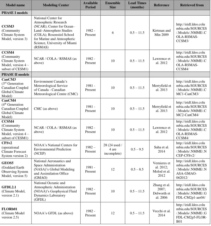
1980s) and real-time forecasts since August 2011. Each model consists of between 6 and 28 “members,”
48
and the forecasts are provided at lead times that range between 0.5 and 11.5 months ahead of the forecast
49
(Table 1). The two key advantages of the NMME, in comparison with other projects, are that the data are
50
made freely available and that the focus is not just on retrospective forecasts, but also on real-time
51
information.
52
A central component of the NMME project consists in quantifying model ensemble skill (Kirtman et al., 53
2014) to generate the most reliable climate forecasts. Model accuracy can be measured on several levels,
54
by comparing each model’s individual members, each model’s ensemble mean (of model members), or the
55
multi-model ensemble mean, against the observed climate data. Typically, multi-model means are found to
56
have greater skill than single models (Hagedorn et al., 2005). Such averaging schemes are usually computed
57
either by giving the same weight to each model’s ensemble mean, or by giving equal weight to all members
58
(thus assigning more weight to the models with more members) (e.g., Tian et al., 2014). The first
59
assessments of NMME skill consistently suggest that the multi-model ensemble mean performs as well as,
60
or better than, the best model (Becker et al., 2014, DelSole and Tippett 2014, Wood et al., 2015, Ma et al. 61
2015a, Thober et al., 2015). This increased skill of the NMME multi-model ensemble in contrast with the
62
individual models appears to be related to the addition of new signals (from new models), rather than to the
63
reduction of noise due to model averaging (DelSole et al., 2014).
64
However, because of the broad spatial and temporal scope of the NMME, most analyses of model skill are
65
limited by necessity to specific lead times, regions, or seasons. Global, 1°-by-1° resolution studies tend to
66
focus either on just one model, or on the shortest available lead time. For instance, Jia et al. (2015)
67
characterize the skill of the high-resolution GFDL model FLOR, while Saha et al. (2014) investigate the
4
skill of the NCEP Climate Forecast System (CFSv2) at the global scale. Conversely, Becker et al. (2014)
69
provide a comprehensive analysis of temperature, precipitation, and sea surface temperature forecasts for
70
multiple models at the global scale, but focus mainly on the shortest available lead time. Wang (2014)
71
examines the global skill of NMME precipitation forecasts for the summer months and only at the shortest
72
lead time. Mo and Lettenmaier (2014) interpolate the NMME forecasts bilinearly to a 0.5° grid over the
73
continental United States to evaluate runoff and soil moisture forecasts, but only up to the 3-month lead
74
time.
75
In contrast, analyses of the NMME conducted at the sub-continental scale often allow for a more
76
comprehensive examination of model skill and of the relationship between ensemble forecasts and climate
77
oscillations, and reveal regional agreement between models (Infanti and Kirtman 2015). In the southeastern
78
United States, for example, it is shown that temperature and precipitation forecasts become increasingly
79
skillful in the winter months at short lead times (Infanti and Kirtman, 2014). Studies found that the
80
predictability of precipitation (Mo and Lyon, 2015), and/or temperature (Roundy et al., 2015) and drought
81
(Ma et al., 2015b) generally improves in regions that are significantly affected by El Niño-Southern
82
Oscillation (ENSO). In North America, the highest correlations between temperature/precipitation forecasts
83
and observations are found in the south-east (SE), south-west (SW), and north-west (NW) during strong
84
Eastern Pacific El Niño events (Infanti and Kirtman 2015). Such analyses also help determine which models
85
are the most useful at the regional/seasonal scale; for instance, over continental China, the CFS models
86
performed the best, followed by GFDL and NASA, the Canadian models, with the IRI and CCSM3 models
87
in the final position (Ma et al. 2015b) (see Table 1 for an overview of models and acronyms – note that we
88
did not include IRI’s fourth-generation atmospheric GCM (ECHAM4p5) in our model selection because it
89
no longer issues real-time forecasts). In an analysis of four NMME models over the continental United
90
States and the Atlantic Warm Pool (AWP), the CFSv2 and GFDL models showed the most skill for
91
predicting seasonal rainfall anomalies in the July-October season (Misra and Li, 2014).
92
Thus, despite an increasing number of analyses focused on the quantification of NMME models’ skill, a
93
systematic investigation across different models, regions, seasons, and lead times is still lacking.
94
Additionally, very little is known regarding the skill of these models for forecasting extended periods of
95
high temperature and/or low precipitation leading to drought conditions, as well as extreme precipitation
96
leading to flooding. For instance, we know that most NMME models were not able to forecast the 2012
97
North American drought correctly, while those that correctly predicted its occurrence did so fortuitously,
98
and “for the wrong reason” (Kam et al. 2014). Therefore, a thorough evaluation of the NMME models’
99
ability to forecast the occurrence of different extremes over extended periods of time is also missing.
100
To fill these gaps, the research questions that we address in this study are the following:
5
- At the intraseasonal scale, what is the skill of the eight individual NMME model ensembles in
102
predicting precipitation and temperature patterns, for every available lead time, every month of the
103
year, and for every sub-region of the continental United States? How do their biases compare? Do
104
certain models perform better than others for certain regions, lead times, and months, and does the
105
eight-model ensemble mean outperform the individual models?
106
- At the seasonal scale, what is the ability of these eight models to forecast extended periods of high
107
temperature and low precipitation leading to drought conditions, as well as prolonged periods of
108
extreme precipitation leading to flooding?
109
To answer these questions, we conduct a systematic decomposition of the forecasting skill of the eight
110
individual model ensembles (computed as the mean of all members in each model) as well as of the
eight-111
model ensemble mean (computed by assigning the same weight to each model’s mean), using the NMME
112
forecast data and observed monthly data for verification. Section 2 presents the forecast and observed data,
113
and Section 3 provides an overview of the statistical methods used to perform forecast verification and the
114
diagnosis of each model’s ability to predict seasonal extremes. The results are presented in Section 4, while
115
Section 5 summarizes the main findings and conclusions of the study.
116
2. Data 117
2.1. NMME Temperature and Precipitation Data 118
Here we focus on eight GCMs from the NMME project, for which temperature and precipitation forecasts
119
are available from the early 1980s to the present. The GCMs we consider are: CCSM3 and CCSM4 from
120
NCAR, COLA and RSMAS; CanCM3 and CanCM4 from Environment Canada’s CMC; CM2.1 and
121
FLORb01 from NOAA’s GFDL; GEOS5 from NASA’s GMAO; CFSv2 from NOAA’s NCEP. The
122
characteristics of the different models are summarized in Table 1. Of these models, CCSM3 and CCSM4
123
are from Phase I of the NMME project, while all of the others are from Phase II.
124
The data were downloaded from the IRI/Lamont Doherty Earth Observatory (LDEO) Climate Data Library
125
(http://iridl.ldeo.columbia.edu/) in netCDF format, on a 1.0° latitude by 1.0° longitude grid. Monthly total
126
precipitation (variable name “prec”, in mm/day) and monthly reference mean temperature at 2 meters
127
(variable name “tref”, in Kelvin units) were obtained for all available lead times and ensemble members
128
over the continental United States. Temperature data were converted from Kelvin units to degrees Celsius.
129
For CanCM3, CanCM4, and CFSv2, the hindcast and forecast data were downloaded separately and
130
combined for the analysis. In the case of CFSv2 we used the pentad realtime forecasts which match the
131
pattern of the CFSv2 hindcasts.
6
Data were extracted for each model from netCDF files in R using the ncdf4 package (Pierce, 2014). The
133
files typically contain five dimensions, which are the longitude, latitude, member, lead, and forecast
134
reference time. The number of ensemble members ranges from 6 for COLA to 12 for GEOS5 and
135
FLORb01, and 28 for CFSv2 (Table 1). To limit the scope of the analysis, we consider the mean of each
136
model’s ensemble members, rather than analyze each model member individually. The focus of our analysis
137
is monthly to seasonal predictions, ranging from 0.5 to 11.5 month leads. The term “lead” indicates the
138
period between the forecast initialization time and the month that is predicted (so a “0.5-month lead
139
forecast” refers to a monthly forecast that was made about 15 days ahead of the forecast period). Model
140
forecast lead times vary from 0.5-9.5 months for GEOS5, and up to 11.5 months for all of the other models
141
(Table 1). Here, the expression “forecast reference time” refers to the date when the forecasts were issued
142
(e.g., July 2015).
143
To analyze forecast skill at the regional scale, we define seven major regions of the United States based on
144
the boundaries described in Kunkel et al. (2013), which are a modification of the regions that were originally
145
used in the 2009 National Climate Assessment Report (Karl et al., 2009) by dividing the Great Plains
146
Region into North and South (Figure 1). The NMME data are projected as stacked rasters and cropped to
147
the dimensions of these seven regions using the ‘raster’ package in R (Hijmans, 2015), to extract the mean
148
weighted forecast value of all of the grid cells falling within each region (as defined by the polygons) for
149
every month and lead time.
150
2.2. Reference Temperature and Precipitation Data 151
To verify model skill, we use temperature and precipitation data from the Parameter-elevation Regression
152
on Independent Slopes Model (PRISM) climate mapping system (Daly et al. 2002), which represents the
153
reference dataset for the continental United States. PRISM’s temporal and spatial resolutions are monthly
154
and approximately 4 km. The data are freely available from the web (http://www.prism.
155
oregonstate.edu/index.phtml) and cover the period from 1890 to the present. We divide precipitation
156
monthly totals by the number of days in each historical month to obtain daily values, and to match the units
157
of the NMME models. Extracted precipitation and temperature data time series are plotted against reference
158
PRISM data for every model, region, month, and lead time for verification purposes (see Supplementary 159
materials, pp.2-25).
160
Other studies (e.g., Becker et al., 2014, Infanti and Kirtman, 2014) have used as verification field the station
161
observation–based Global Historical Climatology Network and Climate Anomaly Monitoring System
162
(GHCN+CAMS) for temperature, and the Climate Prediction Center (CPC) global daily Unified Raingauge
163
Database (URD) gauge analysis for precipitation rate. Here we chose to use PRISM data instead because
7
they account for elevation in the interpolation scheme and have a fine spatial resolution. Moreover, they
165
are the official product for the U.S. Department of Agriculture.
166 167 3. Methodology 168 3.1. Forecast verification 169
Different approaches and methods have been developed to quantify the skill of a forecast system. Here we
170
quantify the accuracy of the forecast relative to the climatology (used as reference) using the mean square
171
error (MSE) skill score SSMSE (e.g., Hashino et al. 2007):
172 2 1 x MSE MSE SS
(1) 173where σx represents the standard deviation of the observations. A perfect forecast receives a skill score of
174
1. As the value tends to zero, the forecast skill decreases. A value of 0 indicates that the forecast accuracy
175
is the same as what we would achieve using climatology as our forecast. Negative values indicate that the
176
accuracy is worse than the climatology forecast. The value of SSMSE can be decomposed into three
177
components (Murphy and Winkler 1992):
178 2 2 2
x x f x f fx fx MSESS
(2) 179where ρfx is the correlation coefficient between observations and forecasts and quantifies the degree of linear
180
dependence between the two; µf and µx are the forecast and observation means, respectively; σf represents
181
the standard deviation of the forecasts. Based on this decomposition, the value of the correlation coefficient
182
(or its squared counterpart, the coefficient of determination) reflects the forecast accuracy only in the
183
absence of biases. For this reason, it represents the potential skill (PS), which is the skill we could achieve
184
if there were no biases. Without the quantification of the biases, the forecast skill is inflated. Thus, it is
185
commonly assumed (e.g., Boer et al., 2013, Younas and Tang, 2013) that the difference between the
186
potential and actual skill represents “room for model improvement”; however, as explained by Kumar et
187
al. (2014), there is not necessarily a relationship between the potential and the actual skill of climate models,
188
and assuming that there should be one amounts to expecting that the real-world data should behave
189
identically to the model predictions.
190
The second term in the right hand side of equation (2) quantifies the conditional biases and is referred to as
191
the slope reliability (SREL). The last term quantifies the unconditional biases and it is referred to as the
192
standardized mean error (SME).
8
Forecast verification using the skill score and its decompositions in equation (2) is a diagnostic tool that
194
produces a more realistic quantification of the forecast skill compared to taking the correlation coefficient
195
at face value. Moreover, the decomposition of the skill in different bias sources can provide model
196
developers with feedback about strengths and weaknesses of their models. In general, unconditional biases
197
(large SME) can easily be removed with bias-correction methods (Hashino et al. 2007). Conditional biases
198
(large SREL), on the other hand, may require more sophisticated calibration. However, forecasts with low
199
potential skill (PS) will have limited predictability, even if biases are eliminated.
200
To perform the skill verification of the NMME data, we tailor the PRISM and NMME data to cover the
201
same months between January 1982 and December 2014. The verification is carried out for each model
202
ensemble mean, region, and lead time following the above procedure, as also described in Bradley and
203
Schwartz (2011). A separate skill verification is conducted on the eight-model ensemble mean, which is
204
the mean forecast of all models (where one model already represents the arithmetic mean of its own
205
ensemble members), for each region and lead time.
206
3.2. Extreme event diagnosis 207
The second part of the diagnosis is the assessment of each model’s ability to predict extreme floods and
208
droughts at the seasonal scale. To do this, we investigate the models’ capacity to capture prolonged periods
209
of extreme precipitation and temperature lasting several months. Eight extreme flood and drought events
210
affecting different parts of the continental United States were selected based on their severity and duration.
211
The event had to last at least one full month, and less than a year, so that we might evaluate its predictability
212
for multiple lead times. The severity of the events was evaluated using the NOAA’s Billion Dollar Weather
213
and Climate Disasters Table of Events (https://www.ncdc.noaa.gov/billions/events). The chosen events
214
include four floods (July-August 1993, January-March 1995, June-August 2008, and March 2010) and four
215
droughts (June-August 1988, March-November 2002, March-August 2011, and May-August 2012). For
216
the flood events, we focus on positive precipitation anomalies (high rainfall), and for the droughts, we
217
observe positive temperature anomalies and negative precipitation anomalies (high temperature and lack of
218
rainfall).
219
We first define the extent of each event based on the description given in the Billion Dollar Weather Table.
220
The PRISM data are aggregated over the entire continental United States at the 1°×1° resolution to match
221
the spatial resolution of the NMME data. At each 1-degree pixel and for the period of interest for a given
222
event, we compute the standardized anomalies with respect to the mean and standard deviation computed
223
over the 1983-2014 period (the years 1982 and 2015 are excluded systematically because not all models
224
have a complete forecast for 1982, and 2015 forecast data were not yet available for all events at the time
225
of the analysis). We then extract all the cells with standardized anomalies larger than 1 and smaller than −1
9
(depending on whether we are considering excess temperature/precipitation or lack of rainfall). The
227
resulting raster contains only the grid cells for that event which were “anomalously” high or low with
228
respect to the 1983-2014 climatology. The boundaries of the event are tailored to the locations indicated in
229
the Billion Dollar Weather Table (Figure 2). We then average all the pixels within this identified region for
230
the months characterizing each event (e.g., total rainfall for the June-August 2008, for each year between
231
1983 and 2014) and compute the “domain averaged” standardized anomalies. Confidence intervals are
232
computed around the anomaly for the given extreme event using the approach described in Stedinger et al.
233
(1993, section 18.4.2).
234
Last, we use a similar procedure to calculate the corresponding NMME anomalies within the defined region.
235
One mean (spatially-averaged) model forecast is extracted for the entire region for the selected months
236
between 1983 and 2014, for each lead time. To obtain a seasonal forecast value we compute the sum of
237
forecasts initialized ahead of the entire season. Thus, for an event such as the June-August 2008 flood, the
238
seasonal forecast initialized in June 2008 (just before the event) is calculated as the sum of the 0.5-, the
1.5-239
, and the 2.5-month lead forecasts initialized in June. If we initialize the forecast one month earlier, in May,
240
the forecast can be calculated as the sum of the 1.5-, the 2.5- and the 3.5-month lead forecasts initialized
241
that month. The forecast is calculated for increasingly long initialization times by going back in monthly
242
time steps, as far the available lead times will allow. The resulting seasonal forecasts are then computed as
243
anomalies, to allow a direct comparison with the average PRISM climatological anomaly for the event.
244
4. Results 245
4.1. Regional temperature and precipitation forecast skill 246
4.1.1 Temperature 247
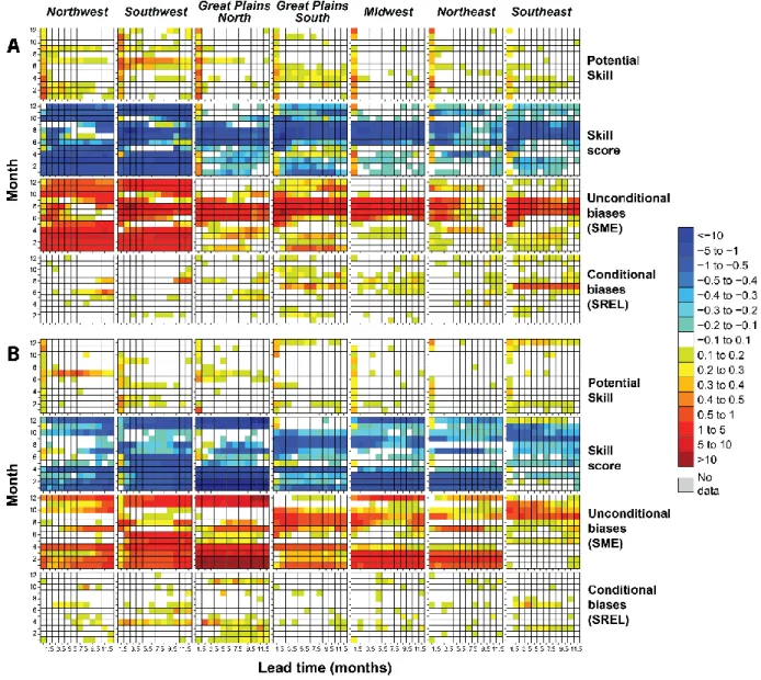
The potential skill of the eight-model ensemble mean, as measured by the squared correlation coefficient
248
between model forecasts and PRISM observations, ranges between 0 and 0.6 (Figure 3a). We find that the
249
highest skill is displayed at the shortest lead time (0.5-month lead) and declines rapidly thereafter, so most
250
regions and months display a skill smaller than 0.1 by the 1.5-month lead time (Figure 3a). The Northwest
251
and Southwest tend to show better skill than the other regions at longer lead times, e.g., over the
January-252
March and June-July periods respectively, possibly because of the good predictability of temperature
253
anomalies arising from ENSO conditions during the same months (see e.g., Wolter and Timlin 2011, and
254
mapping of the likelihood of seasonal extremes by the NOAA/ESRL Physical Science Division at
255
http://www.esrl.noaa.gov/psd/enso/climaterisks/). Other regions such as the Midwest show almost no skill
256
beyond the shortest lead time, possibly because of the weaker relationship with ENSO states.
10
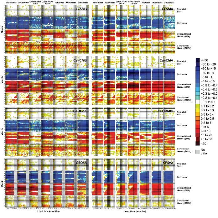
Overall, the ensemble mean displays better ability than any of the individual models, with potential skill
258
maxima that exceed that of any single model (see for example April temperatures in the Midwest at the
0.5-259
lead time, Figures 3-4), in agreement with other assessments of NMME model skill (Infanti and Kirtman 260
2014, Kirtman et al. 2014). There is not one model that clearly outperforms any of the others, although
261
CCSM4, CanCM3, CanCM4, GEOS5 and CFSv2 do display better skill than CCSM3, GFDL2.1, and
262
FLORb01 (Figure 4). The same seasonal and regional patterns can be seen for the individual models as for
263
the ensemble mean, with a clear peak in potential skill in the Southwestern region in the summer months
264
(CCSM4, CanCM4).
265
The actual skill score is relatively low for all models and is mainly driven by the large unconditional biases
266
(SME) in the models. The influence of the unconditional biases on the skill score is clearly detectable in
267
the mirror-image pattern between the two (Figures 3-4). Dark blue colors indicating low skill score are
268
reflected by the dark red colors indicating a high unconditional bias. Overall, the skill score tends to be
269
higher at the shortest lead times. For the ensemble mean, it can be quite high in specific regions such as the
270
Midwest at the 0.5-month lead time during the cold season. Individual models, however, exhibit low skill
271
scores over most regions and months, with values reaching below −10 most of the time (see Supplementary
272
Materials pp.26-29 for additional graphs indicating skill decomposition for the eight-model ensemble mean
273
and for each individual model).
274
The unconditional biases display strong seasonal variability: they tend to be the lowest (white) in most
275
regions in the winter/spring months, and tend to increase dramatically (red) in the summer. By contrast, the
276
Northwest and Southwest exhibit systematically higher biases in the winter and spring (particularly in the
277
model ensemble). Therefore, as a result of this seasonality (e.g., better characterization of initial land surface
278
conditions in the cold seasons), the unconditional biases also show some lead-dependence: during the
279
summer months, they are the highest at the shortest leads (dark red), and decrease progressively with lead
280
time (as is visible in the case of CanCM4/CanCM3, and to a lesser extent CFSv2). These seasonal
281
fluctuations have a notable influence on the overall skill score, and suggest that forecasts made in the
282
summer months could generally be improved by eliminating the unconditional biases.
283
The conditional biases (SREL) tend to range between 0 and 1, and are thus about an order of magnitude
284
lower than the unconditional biases, which are mostly between about 0 and 10. Conditional biases are
285
typically very low during most of the year (Figure 3), and they do not vary notably by lead time for most
286
of the models (Figure 4). One visible exception is the case of CanCM3 and CanCM4, which exhibit a
287
‘stepped’ appearance, so the conditional biases increase (become redder) as lead time increases. These
288
biases in the Canadian models tend to develop more rapidly in the earlier months of the year than in the
11
later months (see CanCM4 conditional biases in the Southwest, for an example). Some of the other models,
290
like GFDL2.1 and GEOS5, also reveal some seasonality in their conditional biases.
291
4.1.2 Precipitation 292
Precipitation forecasts generally have lower potential skill than temperature (Figure 3B), as expected and
293
found in other studies, due to the greater variability in rainfall patterns (e.g., Infanti and Kirtman 2015).
294
The eight-model ensemble mean has better skill than each of the individual models (Figure 3B vs Figure 295
5), and the regions with the highest eight-model potential skill reflect the ability of the most skillful models
296
(e.g., CCSM4, CFSv2 in the Southeast). However, all of the individual models display relatively low
297
potential skill, especially after the 0.5-month lead (consistent with results found by Mo and Lyon (2015)),
298
and little spatial variation on the regional scale (Figure 5). The models with the poorest forecasting ability
299
(e.g., CCSM3 and FLORb01) do not even display potential skill at the 0.5-month lead. Other models (e.g.,
300
CCSM4, the Canadian models, GEOS5 and CFSv2) display some skill at longer lead times, but only for
301
specific months, such as July in the Northwest (for CCSM4, GFDL2.1, CanCM4, and FLORB01), or May
302
in the Southwest (e.g., CanCM4, GEOS5).
303
Similarly to temperature, the skill score for precipitation is mainly driven by unconditional biases in the
304
models: the positive unconditional biases (red patterns) are mirrored by the negative skill score (blue
305
patterns). Overall, however, the skill score for precipitation displays slightly less extreme (positive and
306
negative) values than for temperature. This ‘subdued’ behavior could be caused by the greater variability
307
in precipitation rates (i.e., lower agreement among forecast patterns) in space and time, for different months,
308
lead times, and models. In other words, because of the small spatial scales of precipitation forecasts
309
(compared to temperature), better results might be achieved by focusing on smaller spatial regions than the
310
seven broad regions used here.
311
Interestingly, the seasonality of model skill also varies regionally for precipitation, but is different from the
312
regional patterns for temperature. For the Northwest, Southwest, Great Plains North, Midwest, and
313
Northeast regions, the highest unconditional biases in the precipitation forecasts tend to occur more
314
frequently (lower skill) in the winter months (Figure 3B). The Great Plains South and Southeast regions,
315
on the contrary, display lower unconditional biases (higher skill) in the winter months. This finding is
316
consistent with that of Infanti and Kirtman (2014) for the southeastern United States, and suggests that
317
improved model skill in the winter months may well be related to the influence of ENSO (e.g., Mo and 318
Lyon, 2015, Roundy et al., 2015). In some regions, the unconditional biases tend to increase as the lead
319
time of the forecast increases, so the color maps become progressively redder towards the right side of the
320
plots (e.g., the Northwest region for CanCM3, FLORb01, or CFSv2) (Figure 5). Elsewhere the biases
12
decrease with increasing lead time (e.g., Great Plains South, FLORb01). All eight models display
322
considerable biases, but CCSM3 displays the largest biases, specifically in the Great Plains North region.
323
The conditional biases are again much lower than the unconditional biases, and much more variable,
324
displaying little regularity by month or by lead time. Some months display slightly higher conditional biases
325
(e.g., April or July), but such patterns are infrequent. CCSM3 and CCSM4 have the largest conditional
326
biases (red), followed by GFDL2.1, while the Canadian models, GEOS5 and CFSv2 tend to show lower
327
conditional biases. Regionally, there seem to be slightly greater biases in the Southwest and Great Plains
328
North.
329
4.2. Individual extreme events 330
4.2.1. Floods 331
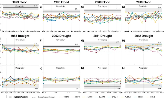
We evaluate the skill of the eight NMME models in predicting four flood events (the 1993 July-August
332
flood, the 1995 January-March flood, the 2008 June-August flood, and March 2010) by comparing the
333
observed climatology (Figure 2, A-D) to the model precipitation forecasts (positive anomalies). As a caveat,
334
it should first be conceded that we do not expect the models to reflect the observed historical precipitation
335
anomalies perfectly over such broad spatial scales, even in the best-case scenarios, because of convection
336
patterns that occur at local scales (and that cannot be captured in the same way as extreme temperature
337
anomalies, which exhibit more spatially-consistent patterns). Overall, results indicate that the four flood
338
events were relatively poorly predicted by all eight models (Figure 6, A-D). The 1993 Midwest flooding
339
stands out as the least poorly forecasted, since all models with the exception of CCSM3 predicted positive
340
anomalies. CanCM4, CCSM4, FLORb01, CFSv2 and CanCM3 all forecasted anomalies that were more
341
than 2 times greater than their own average seasonal value (Figure 6A). However, the actual historical
342
anomaly was much greater than any of the predicted values, at 3.80. Generally speaking, skillful predictions
343
tend to occur in regions that have strong air-sea coupling, so the initial condition of the atmosphere plays
344
an important role in the forecast for several months (Materia et al., 2014). In the case of the 1993 flood, it
345
is likely that the good skill of the models is due to the strength of the El Niño, which displaced the storm
346
track over the central United States, with atmospheric rivers transporting large amounts of moisture from
347
the Gulf of Mexico over the Mississippi River basin (Trenberth and Guillemot, 1996; Lavers and Villarini, 348
2013). The El Niño conditions also likely explain why the ability of the eight models to predict the 1993
349
flood visibly decreased here with initialization time (i.e., the further ahead of the event, the less able the
350
models were to forecast the high rainfall).
351
The other three events were relatively less well forecast, although CFSv2 performed better than all other
352
models in 2008 (Figure 6C), as did FLORb01 in 2010 at the shortest lead time (Figure 6D). The observed
13
event anomalies (PRISM data) were of 2.34, 2.55, and 2.78 while the model forecasts, at best, attained 1.8
354
(GFDL2.1 – 1995 flood), 1.5 (CFSv2 – 2008 flood) and 2.3 (CFSv2 – 2010 flood), but somewhat
355
fortuitously, since some of the highest anomalies were predicted many months ahead of the actual events.
356
In fact, for all three of these flood events (Figure 6B-D), the eight-model ensemble mean is near zero, or
357
below zero, and half of the individual model forecasts predicted a “drier-than-average” season. Figure 6B-358
D indicates that most models fluctuate between positive and negative anomalies, and in 2008 were wrong,
359
predicting a drier-than-average season overall; as for the other flood events, the predicted anomalies were
360
as low as -1.5 (1995 flood - GEOS5), -2.5 (2008 flood – CanCM4), and -2.4 (CFSv2 – 2010 flood). Thus,
361
no model consistently outperformed any of the others, and no single model was reliable in terms of
362
consistently predicting these three flood events (Figure 6B-D).
363
4.2.2. Droughts 364
Droughts tend to develop more slowly than floods, since it can take between five and eight months for the
365
water deficit to drop beneath a certain threshold and begin a drought (Mo, 2011). Hence, skillful
366
intraseasonal to interannual forecasts may prove particularly vital ahead of major drought events.
367
Additionally, droughts also tend to be more predictable than floods because of the influence of the Pacific
368
Decadal Oscillation (PDO) and the Atlantic Multi-decadal Oscillation (AMO) (McCabe et al. 2004) and
369
the effects of land surface/atmosphere coupling (e.g., Koster et al., 2006, Seneviratne et al., 2010). Thus,
370
droughts that are strongly influenced by initial conditions tend to be well-forecast (Roundy and Wood, 371
2014).
372
Here we evaluate the ability of NMME models to predict droughts as high temperature anomalies (excess
373
heat Figure 2, E-H) on the one hand, and low precipitation anomalies (lack of rainfall, Figure 2, I-L) on the
374
other, in comparison with the observed climatology (red shades for excess temperature, blue shades for lack
375
of rain). The comparison between temperature and precipitation predictions for drought events also allows
376
us to determine whether the NMME models are more accurate in predicting excess heat or deficient rainfall,
377
and to what extent temperature actually contributed to drought severity for each of these events. For
378
instance, in the case of the 2014 California drought, it was shown that while low precipitation was the main
379
driver of the event, temperature contributed strongly to intensifying the drought (Shukla et al., 2015).
380
The comparison between observed extreme temperature and observed extreme precipitation anomalies
381
reveals a relatively good overlap in spatial extents (Figure 2) with the exception of the 2002
March-382
November drought, which was also the least predictable of the four droughts (only small isolated parts of
383
the south-east and south-west United States were affected by the positive temperature anomaly, Figure 2F).
384
During droughts, strong precipitation deficits and high heat anomalies tend to occur over the same regions,
385
as was the case during the 1934, 1936, 2011 and 2012 events (Donat et al., 2016). The discrepancies
14
between temperature and precipitation patterns tend to be relatively limited in space and are mainly caused
387
by the noise associated with the precipitation signal; for instance, localized thunderstorms that occur in
388
spring and summer may influence the rainfall anomalies computed for an entire season.
389
Of the four drought events, it appears that the 1988 drought was remarkably well predicted at the shortest
390
initialization time by four models (GEOS5, CFSv2, CanCM3 and GFDL2.1) in terms of high temperature
391
(Figure 6E). The first two of those models actually exceeded the observed anomaly (PRISM=2.1), with
392
forecast values of 2.6 and 2.4. However, the skill of all models decreases rapidly with increasing lead time,
393
indicating that they were unable to predict the event more than one month ahead of its actual occurrence.
394
For the same event, the precipitation forecasts (lack of rainfall) were also relatively successful in June 1988
395
(anomaly values of −3.2 for GEOS5, −2.3 for CFSv2, −2.2 for GFDL2.1, in comparison with the observed
396
−2.8) but the skill declined when predicted further ahead (Figure 6E). CCSM3 performed the least well
397
among all models, while CanCM3 predicted the drought successfully both in terms of temperature and
398
precipitation eight months ahead of the actual event (Figure 6E). Overall, the good predictability of the
399
1988 drought is likely a result of the strong La Niña conditions (e.g., Trenberth and Guillemot, 1996) that
400
occurred in conjunction with a cooling phase of the PDO and the warming phase of the AMO (McCabe et 401
al. 2004).
402
The other three droughts were relatively less well predicted. For 2002, the eight-model ensemble mean is
403
close to climatology (anomaly value around 0), and in the month preceding the event, only GEOS5
404
predicted a positive temperature anomaly of 1.3 vs. 1.77 for the observed climatology, while half of the
405
models actually predicted excess rainfall (Figure 6F). In 2011, the March-August forecasts were slightly
406
more accurate, likely because the drought resulted from a strong La Niña (Seager and Hoerling, 2014) and
407
the mean flow moisture divergence anomalies driven by the negative North Atlantic Oscillation of the
408
previous winter (Seager et al. 2014). GFDL2.1 and FLORB01 both consistently predicted high positive
409
temperature anomalies and low negative precipitation anomalies, even at the longer times before the event,
410
and the eight-model ensemble mean correctly predicted positive/negative anomalies (Figure 6G). Last, the
411
2012 drought was relatively well predicted, with slightly better results for temperature than precipitation.
412
However, contrary to model forecasts, Pacific sea surface temperature (SST) did not play a major role in
413
the drought (Kumar et al. 2013, Hoerling et al. 2013), so the skillful prediction of the drought was in fact
414
"fortuitous, due to the erroneous coupling with pan-Pacific SSTs" (Kam et al. 2014). CanCM3 and CanCM4
415
display good results, but they become less skillful as one approaches the beginning of the event (Figure 416
6H). As suggested by Roundy and Wood (2014), the varying skill of drought forecasts among years implies
417
that they are driven by different mechanisms; atmospheric and land initial conditions, SST and radiative
418
forcing may have varying influences to strengthen/weaken the predictability of events (Jia et al. 2016).
15
Overall, it is interesting to note that the precipitation and temperature forecasts are more similar than one
420
might expect in terms of their ability to forecast the extreme events. In fact, comparing the positive
421
temperature anomalies with the negative precipitation anomalies (Figure 6E-L) indicates that seasonal
422
precipitation and temperature forecasts do tend to reflect one another to a certain extent. When the
423
temperature forecast is skillful, the precipitation forecast tends to be also (e.g., GEOS5 and CanCM3 in
424
1988, or GFDL in 2011, Figure 6G). Likewise, the lack of skill is also mirrored for both temperature and
425
precipitation (e.g., CCSM3 in 2011, Figure 6G).
426
Comparing our results with historical ENSO forecasts suggests that when the land surface/atmosphere
427
interaction is well represented, events tend to be better predicted; hence, the lack of land surface/atmosphere
428
coupling in 2002 may explain why the drought was poorly predicted and why there was little consistency
429
between temperature and precipitation patterns. Therefore, as different models have different abilities
430
depending on seasonality and lead times, strategic multi-model averaging procedures may help increase the
431
forecasting skill of these extreme flood and drought events (e.g., Luo and Wood 2008, Bradley et al. 2015),
432
especially in locations with strong antecedent ENSO signal (e.g., Yuan and Wood, 2013).
433
5. Summary and conclusions 434
By decomposing the skill score of the individual climate models into potential skill, unconditional and
435
conditional biases, we have assessed the strengths and weaknesses of the eight GCM ensemble means and
436
of the eight-model ensemble mean over a range of lead times and initialization months. Our findings provide
437
a diagnostic tool that can give model developers feedback about strengths and weaknesses of their models,
438
and help develop better model-averaging strategies.
439
The results can be summarized as follows:
440
1. The highest potential skill in temperature and precipitation forecasts is displayed at the shortest
441
lead time (0.5 month) and declines rapidly thereafter. For both temperature and precipitation, the
442
potential skill of the eight-model ensemble mean does tend to surpass the skill of the best model
443
within the ensemble. However, there is room for more sophisticated model averaging approaches
444
(i.e., weighting individual models based on their strengths and weaknesses) to improve the model
445
ensemble skill. Overall, the skill score is quite low for all models. The eight-model ensemble
446
displays positive values mostly in the shortest lead times, and there is not one model that clearly
447
outperforms any of the others.
448
2. The biases in these eight models are predominantly unconditional (SME), with strong seasonal-
449
and lead-dependent biases driving the negative skill scores (which are likely dependent on the
450
initialization conditions in different regions and seasons). For temperature, in most regions, the
16
unconditional biases tend to be the lowest in the winter/spring months, and to increase in the
452
summer (while the reverse is true in the Northwest and Southwest). For precipitation, the
453
unconditional biases tend to be the lowest in the summer and fall (while the reverse is true in the
454
Great Plains South and Southeast). Thus, it appears that the skill of these forecasts could be
455
improved by attenuating the unconditional biases that are specific to certain regions and seasons.
456
The conditional biases (SREL) are generally about an order of magnitude smaller than the
457
unconditional biases, and display much more variability across all regions, months, and lead times.
458
3. Overall, the skill of the eight NMME models in predicting four flood events and four drought events
459
shows some inconsistencies. The droughts tend to be better forecast than the floods, even in terms
460
of precipitation, likely because they are more tightly connected to SST-driven climate conditions
461
(McCabe et al. 2004). However, air-sea coupling may also lead to fortuitous forecasts (Kam et al. 462
2014): here, some of the best forecasts occur randomly, sometimes many months ahead of the actual
463
event. While some models were able to predict specific events well, and sometimes months in
464
advance (e.g., CFSv2 for the 1988 drought, or CanCM3 for the 2012 drought), no model
465
consistently outperformed any of the others, or was reliable in terms of consistently predicting
466
events.
467
4. Perhaps more unexpectedly, although average temperature forecasts tend to outperform average
468
precipitation forecasts, we find that the seasonal positive temperature anomalies for the droughts
469
were not more accurately predicted than negative precipitation anomalies. In fact, the ability of the
470
models to forecast drought is remarkably similar in terms of temperature and precipitation.
471
Generally speaking, most forecasted anomalies were at least one standard deviation beneath the
472
observed anomaly, suggesting that the ensemble means of models cannot accurately forecast
473
strongly deviating departures from the climatology over such broad spatial scales. Thus, in future
474
work, extreme values may be better forecast by individual model members and over smaller
475
regions, particularly in the case of precipitation, to avoid the influence of noise arising from
476
localized convective events.
477
These findings highlight some of the strengths and weaknesses of the NMME models across all lead times,
478
months, and for seven major regions of the United States. One of the remaining challenges is our ability to
479
extend precipitation forecast skill beyond the shortest lead time, as is recognized in similar studies (Wood 480
et al. 2015). The overall skill of the eight-model ensemble shows promise for multi-model averaging
481
procedures (e.g., Luo et al 2007, Bradley et al. 2015) that might enable more skillful forecasts at longer
482
lead times. Moreover, future studies should examine whether it is possible to utilize these precipitation and
483
temperature forecasts for impact studies including seasonal discharge forecasting.
484 485
17 Bibliography
486
Becker, E., H. Van den Dool, and Q. Zhang (2014) Predictability and Forecast Skill in NMME. Journal of
487
Climate, 27(15), 5891–5906. http://doi.org/10.1175/JCLI-D-13-00597.1 488
Boer, G. J., V. V. Kharin, and W. J. Merryfield (2013) Decadal predictability and forecast skill. Climate
489
Dynamics, 41(7-8), 1817–1833, http://doi.org/10.1007/s00382-013-1705-0 490
Bradley, A.A., and S.S. Schwartz (2011) Summary verification measures and their interpretation for
491
ensemble forecasts, Monthly Weather Review, 139(9), 3075-3089,
492
http://doi.org/10.1175/2010MWR3305.1 493
Bradley, A.A., M. Habib, and S.S. Schwartz (2015) Climate index weighting of ensemble streamflow
494
forecasts using a simple Bayesian approach. Water Resources Research, 51(9), 1–49.
495
http://doi.org/10.1002/2014WR016811 496
Delsole, T., J. Nattala, and M.K. Tippett (2014) Skill improvement from increased ensemble size and model
497
diversity, Geophysical Research Letters, 41(20), 7331–7342. http://doi.org/10.1002/2014GL060133 498
Daly, C., W.P. Gibson, G.H. Taylor, G.L. Johnson, and P. Pasteris (2002) A knowledge-based approach to
499
the statistical mapping of climate, Climate Research, 22(9), 99-113
500
DelSole, T., and M.K. Tippett, Comparing Forecast Skill (2014) Monthly Weather Review, 142(12), 4658–
501
4678. http://doi.org/10.1175/MWR-D-14-00045.1 502
Delworth, T.L., A.J. Broccoli, A. Rosati, R.J. Stouffer, V. Balaji, J.A. Beesley, W.F. Coke, K.W. Dixon, J.
503
Dunne, K.A. Dunne, and J.W. Durachta (2006) GFDL’s CM2 global coupled climate models. Part I:
504
Formulation and simulation characteristics. Journal of Climate, 19(5), 643–674.
505
http://doi.org/10.1175/JCLI3629.1 506
Donat, M.G., A.D. King, J.T. Overpeck, L.V. Alexander, I. Durre, and D.J. Karoly (2016) Extraordinary
507
heat during the 1930s US Dust Bowl and associated large-scale conditions. Climate Dynamics 46(1-2),
508
413–426 http://doi.org/10.1007/s00382-015-2590-5 509
Hagedorn, R., F.J. Doblas-Reyes, and T.N. Palmer (2005) The rationale behind the success of multi-model
510
ensembles in seasonal forecasting—I. Basic concept, Tellus A, 57(3), 219–233,
511
http://doi.org/10.1111/j.1600-0870.2005.00103.x 512
Hashino, T., A.A. Bradley, and S.S. Schwartz (2007) Evaluation of bias-correction methods for ensemble
513
streamflow volume forecasts, Hydrology and Earth System Sciences Discussions, 3(2), 561-594
18
Hijmans, R. (2015) raster: Geographic Data Analysis and Modeling. R package version 2.4-18.
515
http://CRAN.R-project.org/package=raster 516
Hoerling M., J. Eischeid, A. Kumar, R. Leung, A. Mariotti, K. Mo, S. Schubert and R. Seagar (2013) Causes
517
and predictability of the 2012 Great Plains drought. Bulletin of the American Meteorological Society , 95(2),
518
269-282. http://doi.org/10.1175/BAMS-D-13-00055.1 519
Infanti, J. M., and B.P. Kirtman (2014) Southeastern U.S. Rainfall Prediction in the North American
Multi-520
Model Ensemble. Journal of Hydrometeorology, 15(2), 529–550. http://dx.doi.org/10.1175/JHM-D-13-521
072.1 522
Jia, L., X. Yang, G.A. Vecchi, R.G. Gudgel, T.L. Delworth, A. Rosati, W.F. Stern, A.T. Wittenberg, L.
523
Krishnamurthy, S. Zhang, R. Msadek, S. Kapnick, S. Underwood, Fanrong Zeng, Whit G. Anderson, V.
524
Balaji, and K. Dixon (2015) Improved seasonal prediction of temperature and precipitation over land in a
525
high-resolution GFDL climate model. Journal of Climate, 28(5), 2044–2062.
526
http://dx.doi.org/10.1175/JCLI-D-14-00112.1 527
Jia, L., G.A. Vecchi, X. Yang, R.G. Gudgel, T.L. Delworth, W.F. Stern, K. Paffendorf, S.D. Underwood,
528
and F. Zeng (2016). The Roles of Radiative Forcing, Sea Surface Temperatures, and Atmospheric and Land
529
Initial Conditions in U.S. Summer Warming Episodes. Journal of Climate, 29(11), 4121–4135.
530
http://doi.org/10.1175/JCLI-D-15-0471.1 531
Kam, J., J. Sheffield, X. Yuan, and E.F. Wood (2014) Did a skillful prediction of sea surface temperatures
532
help or hinder forecasting of the 2012 Midwestern US drought? Environmental Research Letters, 9(3),
1-533
9. http://doi.org/10.1088/1748-9326/9/3/034005 534
Karl, T.R., J.M. Melillo, and T.C. Peterson, Eds. (2009) Global Climate Change Impacts in the United
535
States. Cambridge University Press, 189 pp.
536
Kirtman, B.P., and D. Min (2009) Multimodel ensemble ENSO prediction with CCSM and CFS. Monthly
537
Weather Review, 137(9), 2908– 2930. http://dx.doi.org/10.1175/2009MWR2672.1 538
Kirtman, B.P., Du. Min, J.M. Infanti, J.L. Kinter, III, D.A. Paolino, Q. Zhang, H. van den Dool, S. Saha,
539
M. Pena Mendez, E. Becker, P. Peng, P. Tripp, J. Huang, D.G. DeWitt, M.K. Tippett, A.G. Barnston, S. Li,
540
A. Rosati, S.D. Schubert, M. Rienecker, M. Suarez, Z.E. Li, J. Marshak, Y.-K. Lim, J. Tribbia, K. Pegion,
541
W.J. Merryfield, B. Denis, and E.F. Wood (2014) The North American Multimodel Ensemble: Phase-1
542
Seasonal-to-Interannual Prediction; Phase-2 toward Developing Intraseasonal Prediction, Bulletin of the
543
American Meteorological Society, 95(4), 585–601. http://doi.org/10.1175/BAMS-D-12-00050.1 544
19
Koster, R.D., Y.C. Sud, Z. Guo, P.A. Dirmeyer, G. Bonan, K.W. Oleson, E. Chan, D. Verseghy, P. Cox,
545
H. Davies, and E. Kowalczyk (2006) GLACE: The Global Land– Atmosphere Coupling Experiment. Part
546
I: Overview. Journal of Hydrometeology., 7(4), 590–610, http://doi.org/10.1175/JHM510.1.
547
Kumar, A., P. Peng, and M. Chen (2014) Is There a Relationship between Potential and Actual Skill?
548
Monthly Weather Review, 142(6), 2220–2227. http://doi.org/10.1175/MWR-D-13-00287.1 549
Kunkel, K. E., T. R. Karl, H. Brooks, J. Kossin, J. H. Lawrimore, D. Arndt, L. Bosart, D. Changnon, S.L.
550
Cutter, N. Doesken, K. Emanuel, P. Y. Groisman, R.W. Katz, T. Knutson, J. O'brien, C.J. Paciorek, T.C.
551
Peterson, K. Redmond, D. Robinson, J. Trapp, R. Vose, S. Weaver, M. Wehner, K. Wolter, and D.
552
Wuebbles (2013) Monitoring and understanding trends in extreme storms: State of knowledge. Bulletin of
553
the American Meteorological Society, 94(4), 499–514. http://doi.org/10.1175/BAMS-D-11-00262.1 554
Lavers, D.A., and G. Villarini (2013) Atmospheric rivers and flooding over the central United States.
555
Journal of Climate, 26(20): 7829-7836.
556
Lawrence, D.M., K.W. Oleson, M.G. Flanner, C.G. Fletcher, P.J. Lawrence, S. Levis, S.C. Swenson, and
557
G.B. Bonan (2012) The CCSM4 land simulation, 1850-2005: Assessment of surface climate and new
558
capabilities. Journal of Climate 25(7) 2240-2260
559
Luo, L.F., E.F. Wood, and M. Pan (2007) Bayesian merging of multiple climate model forecasts for
560
seasonal hydrological predictions, Journal of Geophysical Research-Atmospheres, 112(D10),
561
http://doi.org/10.1029/2006JD007655 562
Luo, L. F., and E. F. Wood (2008) Use of Bayesian merging techniques in a multimodel seasonal hydrologic
563
ensemble prediction system for the eastern United States, Journal of Hydrometeorology, 9(5), 866–884.
564
Ma, F., A. Ye, X. Deng, Z. Zhou, X. Liu, Q. Duan, J. Xu, C. Miao, Z. Di, and W. Gong (2015a) Evaluating
565
the skill of NMME seasonal precipitation ensemble predictions for 17 hydroclimatic regions in continental
566
China. International Journal of Climatology, 36(1),132–144. http://doi.org/10.1002/joc.4333 567
Ma, F., X. Yuan, and A. Ye (2015b) Seasonal drought predictability and forecast skill over China. Journal
568
of Geophysical Research: Atmospheres, 120(16), 8264–8275. http://doi.org/10.1002/2015JD023185 569
McCabe G.J, M.A. Palecki, and J.L. Betancourt (2004). Pacific and Atlantic Ocean influences on
570
multidecadal drought frequency in the United States. Proceedings of the National Academy of Sciences.
571
101(12), 4136–41 http://doi.org/10.1073/pnas.0306738101 572
Materia S., A. Borrelli, A. Bellucci et al (2014). Impact of atmosphere and land surface initial conditions
573
on seasonal forecasts of global surface temperature. Journal of Climate. 27(24), 9253–9271.
574
http://dx.doi.org/10.1175/JCLI-D-14-00163.1 575
20
Merryfield, W.J., W.-S. Lee, G. J. Boer, V.V. Kharin, J.F. Scinocca, G.M. Flato, R.S. Ajayamohan, J.C.
576
Fyfe, Y. Tang, and S. Polavarapu (2013) The Canadian seasonal to interannual prediction system. Part I:
577
Models and initialization. Monthly Weather Review141(8), 2910-2945. http://doi.org/10.1175/MWR-D-578
12-00216.1 579
Misra, V., and H. Li (2014) The seasonal climate predictability of the Atlantic Warm Pool and its
580
teleconnections, Geophysical Research Letters, 41(2), 661–666, http://doi.org/10.1002/2013GL058740 581
Mo, K. (2011) Drought onset and recovery over the United States, Journal of Geophysical Research,
582
116(D20), http://doi.org/10.1029/2011JD016168 583
Mo, K.C., and D.P. Lettenmaier (2014) Hydrologic prediction over the conterminous United States using
584
the National Multi-Model Ensemble, Journal of Hydrometeorology, 15(4), 1457-1472.
585
http://dx.doi.org/10.1175/JHM-D-13-0197.1 586
Mo, K. C., and B. Lyon (2015) Global Meteorological Drought Prediction using the North American
Multi-587
Model Ensemble. Journal of Hydrometeorology, 16(3), 1409-1424 http://doi.org/10.1175/JHM-D-14-588
0192.1 589
Molod, A., L. Takacs, M. Suarez, J. Bacmeister, I.-S. Song, and A. Eichmann (2012) The GEOS-5
590
atmospheric general circulation model: mean climate and development from MERRA to Fortuna. Technical
591
Report Series on Global Model Data Assimilation, vol 28. NASA Goddard Space Flight Cent., Greenbelt,
592
p 175. 593
Murphy, A.H., and R.L. Winkler (1992) Diagnostic verification of probability forecasts, International
594
Journal of Forecasting, 7(4), 435–455, http://doi.org/10.1016/0169-2070(92)90028-8 595
National Research Council (US) Committee on Assessment of Intraseasonal to Interannual Climate
596
Prediction and Predictability (2010) Assessment of Intraseasonal to Interannual Climate Prediction and
597
Predictability. National Academies Press.
598
Pierce, D. (2014) ncdf4: Interface to Unidata netCDF (version 4 or earlier) format data files. R package
599
version 1.12. http://dwpierce.com/software 600
Roundy, J.K., E. Wood (2015). The Attribution of Land–Atmosphere Interactions on the Seasonal
601
Predictability of Drought, Journal of Hydrometeorology 16.2 (2015): 793-810.
602
http://dx.doi.org/10.1175/JHM-D-14-0121.1 603
Roundy, J.K., X. Yuan, J. Schaake, E.F. Wood (2015) A Framework for Diagnosing Seasonal Prediction
604
through Canonical Event Analysis. Monthly Weather Review, 143(6), 2404–2418.
605
http://doi.org/10.1175/MWR-D-14-00190.1 606
21
Saha, S., S. Moorthi, X. Wu, J. Wang, S. Nadiga, P. Tripp, D. Behringer, Y.-T. Hou, H.-Y. Chuang, M.
607
Iredell, M. Ek, J. Meng, R. Yang, M. Peña Mendez, H. van den Dool, Q. Zhang, W. Wang, M. Chen, and
608
E. Becker (2014) The NCEP Climate Forecast System Version 2. Journal of Climate, 27(6), 2185–2208.
609
http://dx.doi.org/10.1175/JCLI-D-12-00823.1 610
Seager, R., L. Goddard, J. Nakamura, N. Henderson, D.E. Lee. (2014). Dynamical Causes of the 2010/11
611
Texas–Northern Mexico Drought. Journal of Hydrometeorology, 15(1), 39–68.
612
http://doi.org/10.1175/JHM-D-13-024.1 613
Seager, R., M. Hoerling (2014). Atmosphere and ocean origins of North American droughts. Journal of
614
Climate, 27(12), 4581–4606. http://doi.org/10.1175/JCLI-D-13-00329.1 615
Seneviratne, T.C., E.L. Davin, M. Hirschi, E.B. Jaeger, I. Lehner, B, Orlowsky, A.J. Teuling (2010).
616
Investigating soil moisture–climate interactions in a changing climate: A review. Earth‐Science Reviews
617
99(3), 125–161
618
Shukla, S., M. Safeeq, A. AghaKouchak, K. Guan, C. Funk (2015) Temperature impacts on the water year
619
2014 drought in California, Geophysical Research Letters, 42(11), 4384–4393,
620
http://dx.doi.org/10.1002/2015GL063666 621
Stedinger, J.R, R.M, Vogel, and E. Foufoula-Georgiou (1993) Chapter 18, Frequency analysis of extreme
622
events, Handbook of Hydrology. Edited by D.R. Maidment, McGrawHill Book Company, New York.
623
Thober, S., R. Kumar, J. Sheffield, J., Mai, D. Schäfer, and L. Samaniego (2015) Seasonal Soil Moisture
624
Drought Prediction over Europe using the North American Multi-Model Ensemble (NMME). Journal of
625
Hydrometeorology, 16(6), 2329-2344. http://doi.org/10.1175/JHM-D-15-0053.1 626
Tian, D., C.J. Martinez, W.D. Graham, and S. Hwang (2014) Statistical Downscaling Multimodel Forecasts
627
for Seasonal Precipitation and Surface Temperature over the Southeastern United States. Journal of
628
Climate, 27(22), 8384–8411. http://doi.org/10.1175/JCLI-D-13-00481.1 629
Trenberth, K.E., & Guillemot, C.J. (1996). Physical processes involved in the 1988 drought and 1993 floods
630
in North America. Journal of Climate. 9(6), 1288–1298 http://doi.org/10.1175/1520-631
0442(1996)009<1288:PPIITD>2.0.CO;2 632
Vecchi, G.A., T. Delworth, R. Gudgel, S. Kapnick, A. Rosati, A., Wittenberg, F. Zeng, W. Anderson, V.
633
Balaji, K. Dixon, L. Jia, H.-S. Kim, L. Krishnamurthy, R. Msadek, W.F. Stern, S.D. Underwood, G.
634
Villarini, X. Yang, S. Zhang (2014) On the Seasonal Forecasting of Regional Tropical Cyclone Activity.
635
Journal of Climate, 27(21) 7994–8016. http://doi.org/10.1175/JCLI-D-14-00158.1 636
22
Vernieres, G., M.M. Rienecker, R. Kovach, and C. L. Keppenne (2012) The GEOS-iODAS: Description
637
and evaluation. GEOS5 Technical Report GEOS5/TM-2012-104606, Vol 30, 61 pp. 638
Wang, H., Evaluation of monthly precipitation forecasting skill of the National Multi-model Ensemble in
639
the summer season (2014) Hydrological Processes, 28(15), 4472-4486. http://doi.org/10.1002/hyp.9957 640
Wolter, K., M.S. Timlin (2011). El Nino/Southern Oscillation behaviour since 1871 as diagnosed in an
641
extended multivariate ENSO index (MEI.ext). International Journal of Climatology, 31(7), 1074–1087.
642
http://doi.org/10.1002/joc.2336 643
Wood, E F., S.D. Schubert, A.W. Wood, C.D. Peters-Lidard, K. C. Mo, A. Mariotti, and R.S. Pulwarty
644
(2015) Prospects for Advancing Drought Understanding, Monitoring, and Prediction. Journal of
645
Hydrometeorology, 16(4), 1636–1657. http://doi.org/10.1175/JHM-D-14-0164.1 646
Younas, W., and Y. Tang (2013) PNA predictability at various time scales. Journal of Climate, 26(22),
647
9090–9114, http://doi.org/10.1175/ JCLI-D-12-00609.1 648
Yuan, X., and E. F. Wood (2013) Multimodel seasonal forecasting of global drought onset. Geophysical
649
Research Letters, 40(18), 4900–4905. http://doi.org/10.1002/grl.50949 650
Zhang, S., M.J. Harrison, A. Rosati, and A. Wittenberg (2007) System design and evaluation of coupled
651
ensemble data assimilation for global oceanic climate studies. Monthly Weather Review, 135(10), 3541–
652
3564, http://doi.org/10.1175/MWR3466.1 653