In: Applied Soft Computing, Volume 13, Issue 1, pp. 667–675. January, 2013. 1
Utilizing Multiple Pheromones in an Ant-Based
Algorithm for Continuous-Attribute Classification Rule
Discovery
Khalid M. Salamaa,b, Ashraf M. Abdelbara, Fernando E. B. Oterob, Alex A.
Freitasb
a
Dept. of Computer Science & Engineering, American University in Cairo, Cairo, Egypt.
b
School of Computing, University of Kent, Canterbury, UK.
Abstract
The cAnt-Miner algorithm is an Ant Colony Optimization (ACO) based technique for classification rule discovery in problem domains which include continuous attributes. In this paper, we propose several extensions to cAnt-Miner. The main extension is based on the use of multiple pheromone types, one for each class value to be predicted. In the proposed µcAnt-Miner al-gorithm, an ant first selects a class value to be the consequent of a rule and the terms in the antecedent are selected based on the pheromone levels of the selected class value; pheromone update occurs on the corresponding pheromone type of the class value. The pre-selection of a class value also allows the use of more precise measures for the heuristic function and the dynamic discretization of continuous attributes, and further allows for the use of a rule quality measure that directly takes into account the confidence of the rule. Experimental results on 20 benchmark datasets show that our proposed extension improves classification accuracy to a statistically signifi-cant extent compared to cAnt-Miner, and has classification accuracy similar to the well-known Ripper and PART rule induction algorithms.
1. Introduction
Ant Colony Optimization (ACO) [5] is a meta-heuristic for solving com-binatorial optimization problems, inspired by observations of the behavior of ant colonies in nature. Classification rule discovery is an active area of re-search in data mining, and there has been considerable interest in the use of
ACO-based algorithms in classification rule discovery, as reviewed in [8, 15]. Ant-Miner, proposed by Parpinelli et al. [18], is the first ACO algorithm for discovering classification rules of the form:
IF <Term-1> AND <Term-2> AND . . . THEN<Class> ,
where each term is represented as an (attribute =value) pair, and the con-sequent of a rule corresponds to the class value to be predicted. Ant-Miner has been shown to be competitive with well-known classification algorithms, such as C4.5 [19] and CN2 [2]. There has been an increasing interest in improving the Ant-Miner algorithm, resulting in several extensions of the algorithm proposed in the literature [1, 9, 12, 13, 14, 22, 24]. The Ant-Miner algorithm has an important limitation of only being able to process nominal attributes, whilst in practice most real-world classification problems involve both nominal and continuous attributes. Recently, Otero et al. [16] presented an extension, called cAnt-Miner, that handles continuous-valued attributes through the creation of discrete intervals dynamically during the rule construction process.
In this paper, we present an extension ofcAnt-Miner, calledµcAnt-Miner, based on the use of multiple pheromone types, one for each class value to be predicted. An ant first selects a class value to be the consequent of a rule and the antecedent terms are selected based on the pheromone levels associated with the selected class value; pheromone update occurs on the corresponding pheromone type of the class value.
This paper builds on earlier work [20, 21] in which the use of multiple pheromone types was introduced in the context of the original Ant-Miner algorithm. In this paper, we introduce the µcAnt-Miner algorithm which incorporates the idea of multiple pheromone types in the cAnt-Miner algo-rithm, the first ACO classification algorithm able to cope with both nominal and continuous attributes during the rule contruction process. Another new component of µcAnt-Miner is a heuristic function which measures the pre-dictive power of a candidate term to be added to the rule antecedent in the context of the preselected class. This is more precise than the entropy-based heuristic function used in the original cAnt-Miner. Furthermore, we propose a new method for locating the best threshold value of a continuous attribute when selecting the next term to be added to the rule consequent. Again, this method takes advantage of the preselected class in the rule consequent, which leads to a better selection of that threshold value. In addition, we propose a new rule quality evaluation function which aims to give higher preference to rules for which confidence is much higher than support.
The rest of the paper is organized as follows. In Section 2 we present a brief overview of the original Ant-Miner algorithm, followed by an overview of related work on Ant-Miner variations in Section 3 and then a review of the cAnt-Miner algorithm in Section 4. We then describe µcAnt-Miner in Section 5. Sections 6 and 7 discuss our experimental methodology and re-sults, respectively. Finally, conclusions and some future work suggestions are presented in Section 8.
2. Overview of the Ant-Miner Algorithm
Algorithm 1 Pseudo-code of Ant-Miner. Begin Ant-Miner
training set←all training examples;
discovered rule set←φ;
while |training set|> max uncovered examplesdo
InitializeP heromoneAmounts(); CalculateHeuristicV alues(); Rbest←φ; i←0; repeat anti ←Initialize(); ConstructRuleAntecedent(anti); ComputeRuleClass(anti);
Rcurrent ←P runeRule(anti);
Qcurrent ←CalculateRuleQuality(Rcurrent);
U pdateP heromone(Rcurrent);
if Qcurrent > Qbest then
Rbest ←Rcurrent;
end if
i←i+ 1;
until max iterations OR Convergence()
discovered rule set←discovered rule set+Rbest;
training set←training set−Examples(Rbest);
end while End
where rules are created by an ACO-based procedure. The decision com-ponents in the construction graph of Ant-Miner are the available predictor attribute-value pairs representing terms in the form of (attribute, operator, value) to be used to create the antecedents of rules. As the Ant-Miner algorithm only works with nominal attributes, the only available operator is “=” (equal-ity operator)—although the use of a logical negation operator in the an-tecedents of rules was explored in the Ant-Miner extension proposed in [20]. Continuous attributes, if present, must be discretized in a preprocessing step. A high-level pseudo-code of Ant-Miner is shown in Algorithm 1.
In essence, Ant-Miner consists of two nested loops: an outer loop (while
loop) where a single rule per iteration is added to the discovered list of rules— which is initialized empty—and an inner loop (repeat−until loop) where an ACO-based procedure is used to create a rule. In the rule construction process, each ant in the colony attempts to create a rule by selecting the terms for its antecedent probabilistically according to the following state transition function: Pij = ηij ·τij Pa r=1 Pbr s=1(ηrs·τrs) , (1)
where Pij is the probability of selecting the term (attributei = valuej)
(de-noted termij), a is the total number of attributes, and br is the number of
values in the domain of the r-th attribute. As shown in Eq. (1), the prob-ability of choosing termij depends on two factors: 1) the value ηij, which is
the value of a problem-dependent heuristic function; 2) the value τij, which
is the amount of pheromone deposited on termij. The value of the heuristic
function η involves information gain of the term [19] and is computed as follows: ηij = log2(m)−entropy(Tij) Pa r=1 Pbr s=1(log2(k)−entropy(Trs)) , (2)
where the measure of entropy for termij is calculated as:
entropy(Tij) =− m X k=1 |Tijk| |Tij| ! ·log2 |Tijk| |Tij| ! , (3)
where a is the total number of attributes, br is the number of values in the
domain of the r-th attribute, m is the number of classes, |Tij| is the total
(which we will refer to as training set partition Tij), and |Tijw|is the number
of examples in partition Tij that have classw.
An ant continues to add terms to the current rule until all the attributes have been used—given that the antecedent of a rule cannot have more than one term of the same attribute—or until adding any of the remaining terms would make the rule cover less than min examples per rule training exam-ples. Then, the consequent of the rule is chosen by computing the class value with the maximum number of occurrences in the set of training examples satisfying the antecedent of the rule. Finally, the quality of the rule is cal-culated and the pheromone value of each term belonging to the antecedent of the rule is increased according to the quality of the rule. The evaluation function used in Ant-Miner to measure the quality of a rule is [11]:
Q= T P T P +F N | {z } sensitivity × T N T N +F P | {z } specif icity (4)
where TP (true positives) is the number of cases covered by the rule and labeled by the class predicted by the rule, FP (false positives) is the number of cases covered by the rule and labeled by a class different from the class predicted by the rule, FN (false negatives) is the number of cases that are not covered by the rule but are labeled by the class predicted by the rule, and TN (true negatives) is the number of cases that are not covered by the rule and are not labeled by the class predicted by the rule.
After updating the pheromone values for used terms, all pheromone values are normalized to simulate pheromone evaporation. The best rule created by the ACO-based procedure, according to the quality measure, is then added to the list of discovered rules, and the examples covered by that rule are removed from the training set.
The aforementioned set of steps is considered an iteration of the outer loop and is repeated until the number of examples remaining in the training set becomes less than or equal to a user-defined max uncovered examples parameter value. A default rule (with no antecedent) is added at the end to simply predict the majority class in the set of uncovered training examples— that is, the set of examples that are not covered by any discovered rule.
For further details about the original Ant-Miner algorithm, the reader is referred to [18].
3. Related Work
In [1], Chan and Freitas proposed a new rule pruning procedure for Ant-Miner that led to the discovery of simpler (shorter) rules and improved the computational time in datasets with a large number of attributes, although in some datasets this led to a smaller predictive accuracy. Liu et al. presented two extensions: AntMiner2 [12] and AntMiner3 [13]. AntMiner2 [12] employs a density-based heuristic function for calculating the heuristic value for a term, while AntMiner3 [13] is based on a new state transition approach. A pseudorandom proportional transition rule was investigated by Wang in [26]. Smaldon and Freitas [22] introduced the idea of selecting the rule con-sequent class before rule construction — this idea is the inspiration for our multi-pheromone approach — and producing an unordered rule set. Their approach was based on constructing rules for each class separately: an ex-tra For-Each (class value) loop is added as an outer loop for the original algorithm. The consequent of the rule is known by the ant during rule con-struction and does not change. An ant tries to choose terms that improve the accuracy for a rule predicting the class value in the current iteration of the For-Each loop. This approach tends to generate better rules in comparison with the original Ant-Miner, where a term is chosen for a rule in order to decrease entropy in the class distribution of cases matching the rule under construction. However, the entire execution (with the complete training set) is repeated separately for each class value until the number of positive cases (belonging to the current class) remaining in the dataset that have not been covered by the discovered rules is less than or equal tomax uncovered cases. Martens et. al [14] introduced AntMiner+, an Ant-Miner extension which employs pheromone initialization and update procedures based on MAX
-MIN Ant System [23]. In AntMiner+, edges in the construction graph are considered the decision components, and theαand β parameters are also in-cluded as nodes in the construction graph, so that their values are selected, and adapted automatically during the algorithm’s run, not statically set be-fore execution. Moreover, AntMiner+ includes special handling of discrete attributes having ordered values (as opposed to nominal attributes having unordered attributes such as “male” and “female”). Instead of creating a pair hattribute = valuei for each value of an ordinal attribute, AntMiner+ creates two types of bounds that represent the intervals of values to be cho-sen by the ants, allowing for interval rules to be constructed. In addition, an extra vertex group is added at the start of the construction graph containing
class values to allow the selection of class first. This is similar to considering the class as another variable. Rules with different classes can be constructed in the same iteration. Different heuristic values are applied according to the selected class in order to choose the terms that are relevant to the prediction of the selected class. However, pheromone information is shared by all ants constructing rules with different consequents. Like Ant-Miner, AntMiner+ cannot directly process datasets with continuous attributes; such datasets must first be discretized in a pre-processing step.
Galea and Chen [9] presented an ACO approach for the induction of fuzzy rules, named FRANTIC-SRL, which runs several ACO algorithm instances in parallel, each one generates rules for a particular class. Swaminathan [24] proposed an extension to Ant-Miner which enables interval conditions in the rules. For each discrete interval, a node is added to the construction graph and the pheromone value associated to the node is calculated using a mixed kernel probability density function (PDF).
The reader is referred to [15] for a recent survey of swarm intelligence approaches to data mining.
4. How does cAnt-Miner Handle Continuous Attributes?
The cAnt-Miner algorithm was introduced by Otero et al. [16] as an extension of Ant-Miner that can deal with continuous attributes without a discretization preprocessing step. cAnt-Miner creates thresholds on continu-ous attributes’ domain values during the rule construction process, producing terms of the form (ai < v) or (ai ≥v), whereai is a continuous attribute and
v is a threshold value dynamically generated using binary discretization [6]. This is accomplished by applying the following extensions to the Ant-Miner algorithm.
In the construction graph of Ant-Miner, nodes represent terms in the form (attributei =valueij) to be selected to create the antecedent of a rule
(where valueij is the j-th value of the i-th nominal attribute). In
cAnt-Miner, nodes for each continuous attribute are added to the construction graph and connected to all other nodes. Note that continuous attribute nodes do not represent valid terms, as they do not have a relational operator and an associated value. Both operator and value are determined dynamically when an ant selects a continuous attribute node as the next term to be added to the antecedent of a rule.
In order to calculate the heuristic value for a continuous attribute ai
based on its entropy, as in Eq. (2), it is necessary to select a threshold value
v from its domain to dynamically partition the continuous attribute ai into
two intervals: ai < v and ai ≥ v. A threshold value is one of the boundary
points of ai. As defined in [6], a value T in the range of ai is a boundary
point if in the sequence of examples sorted by the value ofai, there exist two
examples e1, e2 ∈ S having different classes (where S is the set of examples in the training set), such that ai(e1)< T < ai(e2); and there exists no other
example `e∈S such that ai(e1)< ai(`e)< ai(e2). The best threshold value is
the boundary point v that minimizes the entropy of the partition, given by:
entropy(ai, v) =
|Sai<v|
|S| ·entropy(Sai<v) +
|Sai≥v|
|S| ·entropy(Sai≥v), (5)
where|Sai<v|is the number of examples in the partitionai < vof the training
set, |Sai≥v| is the number of examples in the partition ai ≥v of the training
set and |S| is the size of the training set. The values entropy(Sai<v) and
entropy(Sai≥v) are computed as in Eq. (3). When the best threshold value
vbest is located, the heuristic value to be associated with the continuous
at-tribute ai corresponds to the minimum entropy value of the two generated
partitions (ai < vbest) and (ai ≥vbest).
Accordingly, when an ant is to select a continuous attribute to add as a term in the current partial rule, the relational operator and the value of this term are computed as described above; the threshold value is selected and the relational operator is selected according to the interval with the lowest entropy. However, it is important to note that only examples covered by the current partial rule are considered in the evaluation of threshold values. Therefore, this procedure is repeated each time a new term is added to the current partial rule. This makes the discretization dynamic as the choice of a threshold value is tailored to the current candidate rule [16].
As for pheromone update, pheromone values are associated with the nodes representing continuous attributes, regardless of the operator or threshold values, while with categorical attributes, the pheromone values are associated with the attribute values.
5. The New Multi-Pheromone Based cAnt-Miner
The use of multiple pheromones types was first explored in [20] in the context of the original Ant-Miner algorithm. The motivation behind using
multiple pheromones types is the hypothesis that the selection of terms that are relevant to the prediction of a specific class value leads to better rules than selecting terms simply to reduce the entropy value, which is calculated taking into account all class values. In addition, sharing pheromone between ants constructing rules predicting different class values can negatively affect the quality of the constructed rules, as the terms that lead to constructing a good rule predicting the class valueCxdo not necessarily lead to constructing
a good rule predicting the class value Cy. In this paper, we present a
multi-pheromone extension of the cAnt-Miner algorithm, which we call µc Ant-Miner. The following describes how our µcAnt-Miner algorithm differs from cAnt-Miner, and a high-level pseudocode description of the µcAnt-Miner algorithm is presented in Algorithm 2.
5.1. Multiple Pheromone Types
First, the rule consequent class is chosen before constructing the rule antecedent, so that terms to be chosen in further steps for the rule antecedent would be relevant to classification of the current consequent. Class values are treated as decision components in the construction graph and they are selected probabilistically according to the pheromone amount and heuristic value associated with them. The heuristic value ηk associated with classk is
calculated as below:
ηk =
f req(k)
|T rainingSet| , (6)
where f req(k) denotes the number of occurrences of class k in the current training set.
In addition, we allow each ant to drop and detect multiple types of pheromone, one for each class value. An ant is only influenced by the amount of pheromone deposited for the class value predicted by its rule under construction—i.e., pheromone is not shared between ants construct-ing rules predictconstruct-ing different class values. This allows choosconstruct-ing terms that are only relevant to the previously selected class. This is implemented by replacing the two-dimensional pheromone structure (attribute, value) by a three-dimensional structure (attribute, value, class) for nominal attributes. Therefore, the amount of pheromone type k deposited on termij (τij,k) is
a representation of the quality of termij in the prediction of class k. For
continuous attributes, since their nodes in the construction graph represent only the attributes not the attribute-value pairs, the pheromone structure will be a two-dimensional structure (attribute, class). Similarly, the amount
of pheromone type kdeposited on continuous attribute ai (τi,k) relates to the
quality of the attribute ai in the prediction of class k.
5.2. Heuristic Function
In µcAnt-Miner, we use a heuristic function which directly reflects the predictive power of a given term to the current pre-selected rule class, rather than seeking to reduce the entropy associated with the entire class distri-bution as in the original cAnt-Miner algorithm. This is obtained by using Laplace-corrected confidence as a heuristic function for term selection, as follows:
ηij,k =
|termij,k|+ 1
|termij|+ m
, (7)
where ηij,k is the heuristic fortermij given that class k is selected,|termij,k|
is the number of training examples which include termij and the current
selected class k, |termij| is the number of training examples having termij
and m is the number of classes. The Laplace-corrected confidence is used for both nominal and continuous attributes. However, an interval (using a threshold value and an operator) should be specified to compute the heuristic value using Eq. (7) for a continuous attribute, as described below.
As shown in Algorithm 2, the selection of the class to be predicted by a rule takes place before antecedent construction. At the beginning of the execution of the algorithm, pheromone levels for every class value are initial-ized. Then, the algorithm enters an iterative (while) loop, where heuristic values are calculated for both attribute and class values in the construction graph and a rule is created by the ACO-based rule construction process. As in cAnt-Miner, the best rule is added to the list of discovered rules and the examples covered by that rule are removed from the training set. Finally, the pheromone levels of the class value predicted by the best rule are re-initialized. The re-initialization does not affect pheromone levels associated with other class values. This iterative process is performed until the num-ber of examples in the training set is less than or equal to a user-defined maximum number of uncovered examples.
In the rule construction process (repeat−until loop), an ant constructs a rule as follows. First, the class value to be predicted by the rule is selected probabilistically according to pheromone and heuristic information (Eq. (6)) associated with the different class values. Then, the antecedent of the rule is constructed by selecting terms based on pheromone and heuristic informa-tion (Eq. (7)) associated with the previously selected class value. When a
Algorithm 2 Pseudo-code ofµcAnt-Miner. Begin µcAnt-Miner
training set←all training examples;
discovered rule set←φ;
InitializeP heromoneAmounts();
while |training set|> max uncovered examplesdo
CalculateHeuristicV alues(); Rbest←φ; i←0; repeat anti ←Initialize(); SelectRuleClass(anti); ConstructRuleAntecedent(anti);
Rcurrent ←P runeRule(anti);
Qcurrent ←CalculateRuleQuality(Rcurrent);
U pdateP heromone(Rcurrent);
if Qcurrent > Qbest then
Rbest ←Rcurrent;
end if
i←i+ 1;
until max iterations OR Convergence()
discovered rule set←discovered rule set+Rbest;
training set←training set−Examples(Rbest);
ReinitializeP heromoneAmounts(Class(Rbest));
end while End
continuous attributes is selected, a term should be constructed in the form of (ai < v) or (ai ≥v) by dynamically generating the thresholdv.
5.3. Dynamic Discretization of Continuous Attributes
InµcAnt-Miner, we propose a new method for locating a threshold value in the continuous attribute domain. Taking advantage of the preselected class value, we aim to select a threshold value that generates partitions with more relevance for predicting that class. This is in contrast to the original version ofcAnt-Miner, where the threshold value is selected only to minimize the entropy among the classes. In essence, we calculate a “discrimination” value for each value v in the boundary points of the continuous attribute ai
given class k, as follows:
disc(ai, v, k) = |Q(Sai<v, k)−Q(Sai≥v, k)|, (8)
whereQ(Sai<v, k) andQ(Sai≥v, k) represent the quality of intervalsSai<v and
Sai≥v respectively with respect to the pre-selected classk, and are calculated
as follows:
Q(Sai<v, k) =supp(Sai<v, k)×conf(Sai<v, k), (9)
Q(Sai≥v, k) =supp(Sai≥v, k)×conf(Sai≥v, k), (10)
where supp(Sai<v, k) and conf(Sai<v, k) denote the support and confidence,
respectively, of the interval (ai < v) in the context of class k. More precisely,
supp(Sai<v, k) represents the ratio of the number of examples where the
at-tributeai has a value less thanv and is labeled by classkto the total number
of examples in the current training set, conf(Sai<v, k) represents the ratio of
the number of examples where the attribute ai has a value less than v and
is labeled by class k to the number of examples having attributeai less than
v. The idea behind Equations (9-10) is that the quality of an interval should be proportional to its support, and also proportional to its confidence.
As shown in Eq. (8), we calculate the absolute difference in quality (mea-sured in terms of support and confidence) between the upper and the lower intervals of the candidate value vi. The idea is to select the threshold value
vbest that maximizes the quality discrimination—with respect to the current
selected class value—between the two intervals. After the threshold that produces the highest quality discrimination value is located, we select the relational operator that produces the interval with the higher confidence,
i.e. if conf(Sai<vbest, k) > conf(Sai≥vbest, k), then the generated term would
be (ai < vbest), else it would be (ai ≥ vbest). Finally, the Laplace-corrected
confidence is computed for the interval with the higher confidence, so that a heuristic value is produced for continuous attribute node ai in the
construc-tion graph.
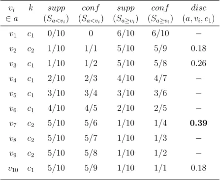
Table 1: Threshold Selection Calculations Example inµcAnt-Miner.
vi k supp conf supp conf disc
∈a (Sa<vi) (Sa<vi) (Sa≥vi) (Sa≥vi) (a, vi, c1) v1 c1 0/10 0 6/10 6/10 − v2 c2 1/10 1/1 5/10 5/9 0.18 v3 c1 1/10 1/2 5/10 5/8 0.26 v4 c1 2/10 2/3 4/10 4/7 − v5 c1 3/10 3/4 3/10 3/6 − v6 c1 4/10 4/5 2/10 2/5 − v7 c2 5/10 5/6 1/10 1/4 0.39 v8 c2 5/10 5/7 1/10 1/3 − v9 c2 5/10 5/8 1/10 1/2 − v10 c1 5/10 5/9 1/10 1/1 0.18
Example. For illustration, Table 1 shows a numerical example of the calculations needed to locate the best threshold for continuous attribute a. Assume that the current partial rule covers the ten examples in the table. The class of each example is indicated in the column labeled k. The class value c1 is selected for the current rule consequent. In order to locate the
best threshold vbest for attribute a, we sort the examples by the value of
attribute a. Then we calculate the quality discrimination value for each boundary point, using Eq. (8). In this example, the boundary values are
{v2, v3, v7, v10}. Since v7 has the highest discrimination value (0.39), it is selected as a threshold. Further, since the confidence value of interval Sa<v7
is higher than the confidence value of intervalSa≥v6, the generated term would
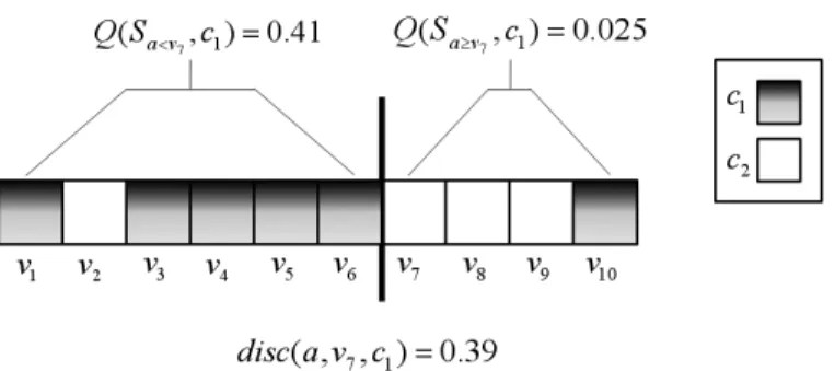
Figure 1: Example illustrating the dynamic discretization process, based on the values shown in Table 1. The array of shaded and unshaded squares represents the 10 training examples of Table 1 sorted ascendingly by the value of attributea. The shaded squares are the examples labeled by the class c1 and the unshaded squares are labeled byc2. As can be seen from the figure,Sa<v7 has the highest concentration of shaded squares (examples
labeled by c1) while Sa≥v7 has the lowest concentration of shaded squares. This makes
v7 the best discrimination value and it would be selected as a threshold for dynamic discretization according to Equation (8).
value for attribute a and it would be selected as a threshold for dynamic discretization according to Equation (8).
We note that the number of boundary points for selecting the threshold in µcAnt-Miner is generally less than or equal to the number of boundary points incAnt-Miner. In µcAnt-Miner, we are only interested in a boundary point T in the range ofai, given that classk is selected, if in the sequence of
examples sorted by the value ofai, there are two examples e1, e2 ∈S having
different classes, such that ai(e1) < T < ai(e2) and one of these two classes
is k. Therefore, the time needed for locating the threshold vbest is reduced,
since fewer candidate boundary points need to be evaluated. 5.4. Rule Pruning
In µcAnt-Miner, some alterations were made to the rule pruning process take advantage of the pre-selection of the rule consequent class and the use of multiple pheromone types. Rule pruning involves speculatively removing each term in turn and evaluating the quality of the rule without that term, then considering the rule with the removed terms having the largest increase in rule quality. This process is repeated until there is no increase in rule qual-ity. In cAnt-Miner, a new consequent – the class with the highest occurrence among all cases covered by the rule – is assigned to the rule after each term is speculatively removed. In contrast, in µcAnt-Miner, the consequent remains
unchanged during the pruning processing, and so the rule pruning procedure is simplified. After each term is removed, there is no need to compute the class with the highest occurrence among all cases covered by the reduced rule. This is because all the terms in the rule antecedent are selected based on the consequent class, so it is certain that the current class produces the highest quality with the current terms compared to other classes.
5.5. Rule Quality Evaluation Function
InµcAnt-Miner, instead ofcAnt-Miner’s rule quality evaluation function (Eq. (4)), we would like to use an evaluation function that takes advantage of the pre-selection of class value and directly takes into account the confidence of the rule. In addition to favoring high-confidence rules, we would also like to favor rules with high support, in order to avoid over-fitting. We might consider the following evaluation function (first used in AntMiner+ [14]):
Q(Rt) =supp(Rt) +conf(Rt), (11)
where supp(Rt) represents the ratio of the number of examples that match
Rt’s antecedent and are labeled by its class to the total number of examples in
the training set, andconf(Rt) represents the ratio of the number of examples
that match rule Rt’s antecedent and are labeled by its class to the total
number of examples that match Rt’s antecedent.
However, instead of using the evaluation function in Eq. (11), we use the following conditional evaluation function, that aims to attach higher quality to rules in which confidence is much higher than support.
Q(Rt) =
( supp(Rt) +conf(Rt) if conf(Rt)≥3supp(Rt)
orconf(Rt) = 1 [case 1]
0.5supp(Rt) +conf(Rt) otherwise ifconf(Rt)≥2supp(Rt) [case 2]
conf(Rt) otherwise [case 3]
(12) The motivation behind the evaluation function of Equation (12) is the following. The evaluation function of Equation (11) assigns equal quality to a rule R1 with a support of 0.2 and a confidence of 0.7, and a rule R2 with
a support of 0.7 and a confidence of 0.2. But, in fact, R2 is quite poor: its antecedent is satisfied by 70% of the training set, but its misclassification rate is 80%—which means that is misclassifies a majority of the training set. Meanwhile, R1 only covers 20% of the training set, but it has a correct classification rate of 70% for this small portion of the dataset that it covers. Thus, the idea behind our proposed evaluation function is that we would like
to promote rules whose confidence is significantly higher than their support— ideally at least three times higher.
Therefore, case 1 of Equation (12) includes the case where confidence is three times or more higher than the support, or where the confidence is 100% regardless of support. In case 2, the ratio of confidence to support is higher than 2 but lower than 3. This is not an ideal rule—therefore, we attach a coefficient of one-half to support so that a rule R3 with a support of 0.7 and a confidence of 0.25 will have a lower quality evaluation than a rule R4 with a support of 0.25 and a confidence of 0.7. In addition, the maximum quality evaluation for a case 2 rule is 1.5 while a case 1 rule can have an evaluation as high as 2. Finally, case 3 includes rules that are not preferred—rules in which the ratio of confidence to support is less than 2. In case 3, the evaluation function does not include support and is based entirely on confidence (which means the maximum quality evaluation would be 1). A rule that is evaluated under case 3 is likely to have a relatively poor evaluation compared to other rules.
Note that the rule quality Q(Rt) computed via Eq. (12) is the amount of
pheromone to be deposited on the class label and the terms of the rule Rt.
6. Experimental Methodology
The performance ofµcAnt-Miner was evaluated using twenty well-known publicly-available datasets from the UCI dataset repository [25]. We compare the performance of µcAnt-Miner against the original version of cAnt-Miner (proposed in [16]) as well as two well-known classification algorithms from the Weka workbench [27], namely JRip (Weka’s RIPPER [3] implementation) and PART [7].
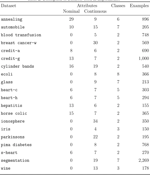
The main characteristics of the datasets used in the experiments are shown in Table 2. Some of the selected datasets only contain continuous attributes, while others contain a combination of nominal and continuous attributes. Nine of the used datasets have more than two values in the do-main of the class attribute, while the redo-mainder have a binary-valued class attribute.
Ten-fold cross validation was used in all experiments by splitting the dataset into 10 stratified folds of approximately the same size (10% of the examples in each fold), with roughly the same distribution of classes in each fold. Then, for JRip and PART, which are deterministic algorithms, each algorithm is run 10 times, each time with a different pair of training and
Table 2: Description of Datasets Used in Experiments.
Dataset Attributes Classes Examples
Nominal Continuous annealing 29 9 6 896 automobile 10 15 7 205 blood transfusion 0 5 2 748 breast cancer-w 0 30 2 569 credit-a 8 6 2 690 credit-g 13 7 2 1,000 cylinder bands 16 19 2 540 ecoli 0 8 8 366 glass 0 9 7 213 heart-c 6 7 5 303 heart-h 6 7 5 294 hepatitis 13 6 2 155 horse colic 15 7 2 365 ionosphere 0 34 2 350 iris 0 4 3 150 parkinsons 0 22 2 195 pima diabetes 0 8 2 768 s-heart 6 7 2 270 segmentation 0 19 7 2,269 wine 0 13 3 178
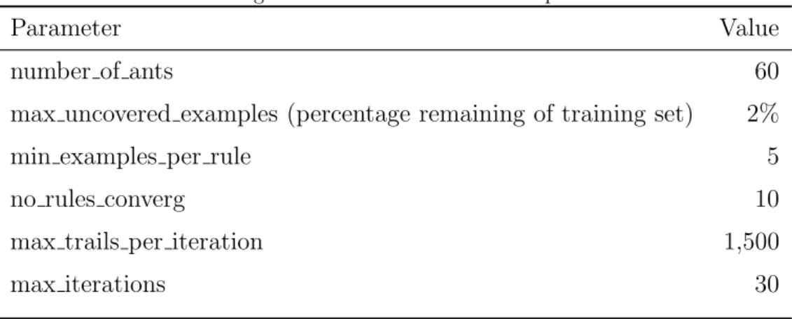
Table 3: Algorithm Parameters Used in Experiments.
Parameter Value
number of ants 60
max uncovered examples (percentage remaining of training set) 2%
min examples per rule 5
no rules converg 10
max trails per iteration 1,500
max iterations 30
testing sets, i.e, each time a different fold is used as the testing set and the other nine folds are merged and used as the training set. Since the ant colony algorithms are non-deterministic, each of those two algorithms was run 15 times per each training/testing set pair—using different random seeds—and the average was taken. Thus, for the ant colony algorithms, the total number of runs for each dataset is 150 (10 training/testing set pairs, each used 15 times). The number of rules generated (which represents a measure of the simplicity of the output), as well as the predictive accuracy of the generated rules were recorded to evaluate the quality of the produced classification models. The parameter settings used in the experiments are shown in Table 3.
7. Experimental Results
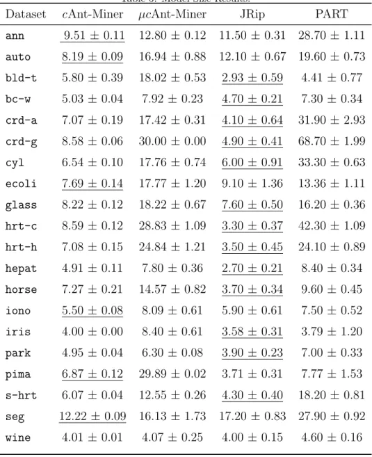
Tables 4 and 5 show the experimental results for predictive accuracy and model size (represented by the number of generated rules), respectively, for cAnt-Miner, µcAnt-Miner, JRip, and PART. For each dataset, each ta-ble shows the mean and standard deviation (mean±std. deviation) of the achieved performance measure (predictive accuracy in Table 4, and model size in Table 5). In addition, an entry is underlined if, for the corresponding dataset, the value obtained by the corresponding algorithm is the best among the four evaluated algorithms.
As Table 4 indicates,µcAnt-Miner outperformed cAnt-Miner in the pre-dictive accuracy of the generated classification rule model in all but 4 datasets, namely cylinder, ecoli, horse, and heart-h. In addition, µcAnt-Miner
Table 4: Predictive Accuracy Results.
Dataset cAnt-Miner µcAnt-Miner JRip PART ann 89.32 ± 1.04 92.84 ±0.56 94.87 ± 0.59 94.63± 0.68 auto 67.52 ± 2.57 71.04 ±1.52 68.69 ± 2.45 76.64± 3.08 bld-t 73.36 ± 0.67 74.93 ±1.72 77.63 ± 3.95 77.89± 3.13 bc-w 93.26 ± 0.65 94.11 ±0.61 94.20 ± 0.98 95.08± 1.00 crd-a 85.30 ± 0.93 86.70 ±0.84 85.51 ± 1.46 84.35± 1.08 crd-g 70.66 ± 1.00 71.11 ±0.20 72.20 ± 1.46 70.40± 1.60 cyl 71.30 ± 0.76 70.51 ±1.15 64.29 ± 2.29 74.51± 1.72 ecoli 79.40 ± 1.79 78.61 ±1.86 82.12 ± 4.76 83.62± 3.75 glass 67.44 ± 3.08 68.23 ±2.37 66.54 ± 2.94 65.62± 3.01 hrt-c 55.99 ± 1.42 56.29 ±0.97 54.48 ± 1.59 53.52± 2.37 hrt-h 62.91 ± 1.60 60.41 ±1.83 63.72 ± 0.80 64.64± 3.16 hepat 76.84 ± 3.13 80.27 ±2.04 78.13 ± 2.66 83.25± 3.47 horse 80.45 ± 2.58 70.23 ±2.16 83.54 ± 1.87 82.39± 2.10 iono 87.08 ± 1.49 93.89 ±1.43 90.24 ± 1.23 90.23± 1.44 iris 94.21 ± 0.99 95.65 ±3.27 93.50 ± 3.84 93.02± 3.55 park 87.40 ± 1.83 90.00 ±1.21 88.76 ± 2.37 86.18± 2.02 pima 72.96 ± 1.13 73.43 ±1.30 74.71 ± 2.34 73.35± 2.51 s-hrt 77.88 ± 2.23 79.79 ±1.38 78.52 ± 2.33 75.93± 1.93 seg 93.72 ± 0.38 94.64 ±0.42 94.58 ± 0.51 95.61± 0.32 wine 91.38 ± 1.72 93.82 ±1.69 92.19 ± 2.22 92.75± 1.44
Table 5: Model Size Results.
Dataset cAnt-Miner µcAnt-Miner JRip PART ann 9.51 ± 0.11 12.80 ±0.12 11.50 ± 0.31 28.70± 1.11 auto 8.19 ± 0.09 16.94 ±0.88 12.10 ± 0.67 19.60± 0.73 bld-t 5.80 ± 0.39 18.02 ±0.53 2.93 ± 0.59 4.41 ± 0.77 bc-w 5.03 ± 0.04 7.92 ± 0.23 4.70 ± 0.21 7.30 ± 0.34 crd-a 7.07 ± 0.19 17.42 ±0.31 4.10 ± 0.64 31.90 ± 2.93 crd-g 8.58 ± 0.06 30.00 ±0.00 4.90 ± 0.41 68.70 ± 1.99 cyl 6.54 ± 0.10 17.76 ±0.74 6.00 ± 0.91 33.30 ± 0.63 ecoli 7.69 ± 0.14 17.77 ±1.20 9.10 ± 1.36 13.36 ± 1.11 glass 8.22 ± 0.12 18.22 ±0.67 7.60 ± 0.50 16.20 ± 0.36 hrt-c 8.59 ± 0.12 28.83 ±1.09 3.30 ± 0.37 42.30 ± 1.09 hrt-h 7.08 ± 0.15 24.84 ±1.21 3.50 ± 0.45 24.10 ± 0.89 hepat 4.91 ± 0.11 7.80 ± 0.36 2.70 ± 0.21 8.40 ± 0.34 horse 7.27 ± 0.21 14.57 ±0.82 3.70 ± 0.34 9.60 ± 0.45 iono 5.50 ± 0.08 8.09 ± 0.61 5.90 ± 0.61 7.50 ± 0.52 iris 4.00 ± 0.00 8.40 ± 0.61 3.58 ± 0.31 3.79 ± 1.20 park 4.95 ± 0.04 6.30 ± 0.08 3.90 ± 0.23 7.00 ± 0.33 pima 6.87 ± 0.12 29.89 ±0.02 3.71 ± 0.31 7.77 ± 1.53 s-hrt 6.07 ± 0.04 12.55± 0.26 4.30 ± 0.40 18.20 ± 0.81 seg 12.22 ± 0.09 16.13 ±1.73 17.20 ± 0.83 27.90± 0.92 wine 4.01 ± 0.01 4.07 ± 0.25 4.00 ± 0.15 4.60 ± 0.16
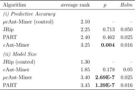
Table 6: Statistical test results according to the non-parametric Friedman test with the Holm’s post-hoc test forα= 0.05.
Algorithm average rank p Holm
(i) Predictive Accuracy
µcAnt-Miner (control) 2.10 – –
JRip 2.25 0.713 0.050
PART 2.40 0.462 0.025
cAnt-Miner 3.25 0.004 0.016 (ii) Model Size
JRip (control) 1.30 – –
cAnt-Miner 1.85 0.178 0.05
µcAnt-Miner 3.40 2.69E-7 0.025
PART 3.45 1.39E-7 0.016
was the overall winner (out of the four algorithms in Table 4) in 8 datasets, whilst PART was the winner in 8 datasets, JRip in just 4 and the original cAnt-Miner was not the winner in any dataset.
As Table 5 indicates, the original cAnt-Miner had the smallest number of rules in 6 datasets, JRip had the smallest number of rules in 13 datasets, and neither µcAnt-Miner nor PART had the smallest model size in any of the datasets.
Table 6 shows the results of the statistical tests according to the non-parametric Friedman test with the Holm’s post-hoc test [4, 10], for both predictive accuracy and model size. For each algorithm, the first column shows its average rank (the lower the average rank the better its perfor-mance), the second column shows the p-value of the statistical test when its average rank is compared to the average rank of the control algorithm (the algorithm with the best rank) and the third column shows Holm’s critical value. Statistically significant differences at the 5% level (corresponding to the cases where thepvalue is lower than the critical value) between the ranks of an algorithm and the control algorithm are tabulated in bold face.
based on predictive accuracy among the four algorithms being compared. On the other hand, in terms of model size, µcAnt-Miner ranked behind JRip and cAnt-Miner, and only slightly better than PART.
The larger models of µcAnt-Miner can be attributed to the quality con-trast intensifier strategy employed by µcAnt-Miner, which tends to prefer rules whose confidence is much higher than their support. As was discussed in Section 5.5, a rule R1 with a confidence of 70% and 20% support will be preferred to another rule R2 with the same confidence but 30% support, and both will be preferred to a third rule R3 with the same confidence and 40%
support. The intuition behind this, as discussed in Section 5.5, was that if
R3 is included in the constructed rule set, it would guarantee that 12% of the training set would be misclassified, while R2 would misclassify 9% of the
training set, andR1 would misclassify 6% of the training set. Of course, the
other side of the coin is that R1 would leave 80% of the training set that would have to be covered by other rules, while R2 and R3 would only leave
70% and 60%, respectively, to be covered by other rules. Thus, a side-effect of this approach is that larger, but more reliable, rule sets will generally be generated.
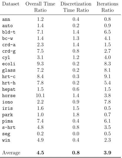
The size of the discovered model also has an effect onµcAnt-Miner’s run-time; on most datasets, µcAnt-Miner tends to have a higher run-time com-pared to cAnt-Miner. The reason for this is that, in addition to discovering a greater number of rules, µcAnt-Miner carries out more iterations before converging on a single rule to be added to the discovered rule list as a result of the class-base structure used for the pheromone matrix, which increases its overall run-time. On the other hand, the discretization process tends to take less time in µcAnt-Miner, because a smaller number of cut points need to be evaluated (as discussed in Section 5.3). Table 7 shows the run-time results for µcAnt-Miner and cAnt-Miner. For each dataset, the table shows the following: the average ratio of the total run-time of µcAnt-Miner to the total run-time of cAnt-Miner, the ratio of the average time spent within a single call of the dynamic discretization process for µcAnt-Miner to that of cAnt-Miner, and the ratio of the average number of iterations per generated rule forµcAnt-Miner to that of cAnt-Miner. The last row of the table shows the average of each column over all datasets. We observe that, on average, the dynamic discretization process takes about 20% less time per call, how-ever, the number of iterations per generated rule is 3.9 times larger, and the total run-time is 4.5 times larger.
Table 7: Execution time results: column 2 shows the ratio of the total execution time of
µcAnt-Miner to the total execution time ofcAnt-Miner, column 3 shows the ratio of the execution time spent within a single call of the dynamic discretization process forµc Ant-Miner to that for cAnt-Miner, and column 4 shows the ratio of the number of iterations per generated rule forµcAnt-Miner to that forcAnt-Miner.
Dataset Overall Time Discretization Iterations Ratio Time Ratio Ratio
ann 1.2 0.4 0.8 auto 1.4 0.2 0.9 bld-t 7.1 1.4 6.5 bc-w 1.4 1.3 4.1 crd-a 2.3 1.4 1.5 crd-g 7.5 0.8 2.7 cyl 3.1 1.2 4.0 ecoli 9.3 0.2 8.3 glass 7.2 0.2 8.1 hrt-c 8.4 0.3 9.1 hrt-h 7.8 0.2 5.4 hepat 1.5 0.6 1.5 horse 10.1 1.4 3.8 iono 2.2 0.9 7.8 iris 1.6 1.5 0.5 park 1.0 1.8 0.7 pima 7.4 0.4 6.1 s-hrt 4.8 0.8 3.5 seg 0.2 0.0 0.5 win 4.9 0.4 2.3 Average 4.5 0.8 3.9
8. Conclusions and Future Work Directions
In this paper, we have proposed a multi-pheromone extension of the cAnt-Miner ACO-based classification algorithm. Our approach allows for multiple pheromone types, one for each class value to be predicted. An ant first selects a class value to be the consequent of a rule and the terms to be added to its antecedent are selected based on the pheromone levels of the selected class value; pheromone update occurs on the correspondent pheromone type of the class value. Furthermore, we propose a new method for threshold selection for the domain of continuous attributes based on quality discrimination between generated intervals, which focuses on the predictive power of the generated term with respect to the selected class. We found, in experimental results on a number of datasets, that the predictive accuracy of our proposed method is better than that of the original cAnt-Miner, to a statistically significant extent. Furthermore, although there is no statistically significant difference in predictive accuracy between our method and Ripper and PART (two state-of-the-art rule induction algorithms), our proposed multi-pheromone version of cAntMiner achieved overall the best predictive accuracy among the four algorithms compared in our experiments.
Otero et al. [17] have recently found that the use of a Minimum De-scription Length (MDL) based discretization scheme combined with using pheromone on the edges of the construction graph can improve the perfor-mance of cAnt-Miner. In future work, we would like to explore combining
µcAnt-Miner with the approaches proposed by Otero et al. [17]. References
[1] A. Chan and A. Freitas, “A new classification-rule pruning procedure for an ant colony algorithm,” Artificial Evolution, Lecture Notes in Com-puter Science, Vol. 3871, pp. 25–36, 2005.
[2] P. Clark and T. Niblett, “The CN2 rule induction algorithm,” Machine Learning, Vol. 4, pp. 261–283, 1989.
[3] W.W. Cohen, “Fast effective rule induction,” Proceedings of the 12th International Conference on Machine Learning, pp. 115-123, 1995. [4] J. Demˇsar, “Statistical comparisons of classifiers over multiple data
[5] M. Dorigo and T. St¨utzle,Ant Colony Optimization, MIT Press, 2004. [6] U. Fayyad and K. Irani, “Multi-interval discretization of
continuous-valued attributes for classification learning,” Proceedings Thirteenth In-ternational Joint Conference on Artificial Intelligence, Morgan Kauf-mann, pp. 1022–1027, 1993.
[7] E. Frank and I.H. Witten, “Generating accurate rule sets without global optimization,” Proceedings of the Fifteenth International Conference on Machine Learning, pp. 144-151, 1998.
[8] A.A. Freitas, R.S. Parpinelli, and H.S. Lopes, “Ant colony algorithms for data classification,” In: M. Khosrou-Pour (Ed.), Encyclopedia of In-formation Science and Technology, second edition, InIn-formation Science Reference, pp. 154-159, 2008.
[9] M. Galea and Q. Shen, “Simultaneous ant colony optimization algo-rithms for learning linguistic fuzzy rules,” Swarm Intelligence in Data Mining, Springer-Verlag, pp. 75–99, 2006
[10] S. Garc´ıa and F. Herrera, “An extension on “Statistical comparisons of classifiers over multiple data sets” for all pairwise comparisons,” Ma-chine Learning Research, Vol. 9, pp. 2677-2694, 2008.
[11] H. Jaiwei and M. Kamber, Data Mining: Concepts and Techniques, Morgan Kaufmann, San Mateo, CA, 2006.
[12] B. Liu, H. A. Abbass, and R. McKay, “Density-based heuristic for rule discovery with ant-miner,” in Proc. 6th Australasia-Japan Joint Work-shop on Intell. Evol. Syst., pp. 180–184, 2002.
[13] B. Liu, H. A. Abbass, and R. McKay, “Classification rule discovery with ant colony optimization,”Proceedings IEEE/WIC Int. Conf. Intell. Agent Technol., pp. 83–88, 2003.
[14] D. Martens, M. De Backer, R. Haesen, J. Vanthienen, M. Snoeck, and B. Baesens, “Classification with ant colony optimization,” IEEE Trans-actions on Evolutionary Computation., Vol. 11, pp. 651–665, 2007. [15] D. Martens, B. Baesens, and T. Fawcett, “Editorial survey: swarm
in-telligence for data mining,” Machine Learning, Vol. 82, No. 1, pp. 1–42, 2011.
[16] F. Otero, A. Freitas, and C.G. Johnson, “cAnt-Miner: an ant colony classification algorithm to cope with continuous attributes,”Ant Colony Optimization and Swarm Intelligence, Lecture Notes in Computer Sci-ence, Vol. 5217, pp. 48–59, 2008.
[17] F. Otero, A. Freitas, and C.G. Johnson, “Handling continuous attributes in ant colony classification algorithms,” IEEE Symposium on Computa-tional Intelligence and Data Mining, CIDM ’09, pp. 225–2317, 2009. [18] R. S. Parpinelli, H. S. Lopes, and A. Freitas, “Data mining with an
ant colony optimization algorithm,”IEEE Transactions on Evolutionary Computation, Vol. 6, pp. 321–332, 2002.
[19] J. R. Quinlan, C4.5: Programs for Machine Learning, Morgan Kauf-mann, San Mateo, CA, 1993.
[20] K. M. Salama and A. M. Abdelbar, “Extensions to the Ant-Miner clas-sification rule discovery algorithm,” Proceedings ANTS 2010: Seventh International Conference on Swarm Intelligence, pp. 43–50, 2010. [21] K.M. Salama, A.M. Abdelbar, and A.A. Freitas, “Multiple pheromone
types and other extensions to the Ant-Miner classification rule discovery algorithm,” Swarm Intelligence, Vol. 5, No. 3-4, pp. 149–182, 2011. [22] J. Smaldon and A. Freitas, “A new version of the Ant-Miner algorithm
discovering unordered rule sets,” Proceedings Genetic and Evolutionary Computation Conference (GECCO), pp. 43–50, 2006.
[23] T. St¨utzle, and H. Hoos, MAX-MIN ant system. Future Generation Computer Systems, Vol. 16, No. 8, pp. 889–914, 2000.
[24] S. Swaminathan, Rule Induction Using Ant Colony Optimization for Mixed Variable Attributes, Master’s Thesis, Texas Tech University, 2006.
[25] UCI Repository of Machine Learning Databases, retrieved August 2010 from http://www.ics.uci.edu/~mlearn/MLRepository.html
[26] Z. Wang, and B. Feng, “Classification rule mining with an improved ant colony algorithm,” Advances in Artificial Intelligence, Lecture Notes in Computer Science, Vol. 3339, pp. 357-367, 2004.
[27] H. Witten and E. Frank, Data Mining: Practical Machine Learning Tools and Techniques, 2nd edition, Morgan Kaufmann, San Mateo, CA, 2005.