Information Extraction from Biomedical Text Using Machine Learning

(1)

San Jose State University San Jose State University

SJSU ScholarWorks

Master's Projects Master's Theses and Graduate Research Fall 12-16-2019

Information Extraction from Biomedical Text Using Machine

Learning

Deepti Garg

Follow this and additional works at: https://scholarworks.sjsu.edu/etd_projects

Part of the Artificial Intelligence and Robotics Commons, and the Databases and Information Systems Commons

(2)

Information Extraction from Biomedical Text Using Machine Learning

A Project Presented to

The Faculty of the Department of Computer Science San José State University

In Partial Fulfillment

of the Requirements for the Degree Master of Science

by Deepti Garg December 2019

(3)

(4)

The Designated Project Committee Approves the Project Titled Information Extraction from Biomedical Text Using Machine Learning

by Deepti Garg

APPROVED FOR THE DEPARTMENT OF COMPUTER SCIENCE SAN JOSÉ STATE UNIVERSITY

December 2019

Dr. Wendy Lee Department of Computer Science, San Jose State University Dr. Natalia Khuri Department of Computer Science, Wake Forest University Dr. Mike Wu Department of Computer Science, San Jose State University

(5)

ABSTRACT

Information Extraction from Biomedical Text Using Machine Learning by Deepti Garg

Inadequate drug experimental data and the use of unlicensed drugs may cause adverse drug reactions, especially in pediatric populations. Every year the U.S. Food and Drug Administration approves human prescription drugs for marketing. The labels associated with these drugs include information about clinical trials and drug response in pediatric population. In order for doctors to make an informed decision about the safety and effectiveness of these drugs for children, there is a need to analyze complex and often unstructured drug labels. In this work, first, an exploratory analysis of drug labels using a Natural Language Processing pipeline is performed. Second, Machine Learning algorithms have been employed to build baseline binary classification models to identify pediatric text in unstructured drug labels. Third, a series of experiments have been executed to evaluate the accuracy of the model. The prototype is able to classify pediatrics-related text with a recall of 0.93 and precision of 0.86.

(6)

ACKNOWLEDGMENTS

I thank Dr. Natalia Khuri for her immense guidance, support and honest critique throughout my work. I extend my gratitude to Dr. Wendy Lee and Dr. Mike Wu for their valuable review and feed back. I also thank Shantanu Deshmukh and Maxim Drojjin for helpful discussions. Lastly, I thank my family and friends who have supported my academic endeavour throughout the past two years.

(7)

TABLE OF CONTENTS

CHAPTER

1 Introduction . . . 1

1.1 Information Extraction . . . 1

1.2 Named Entity Recognition . . . 2

1.3 Relation Extraction . . . 3

1.4 Challenges in working with biomedical texts . . . 4

2 Related Work . . . 6

2.1 Rule-based Methods . . . 6

2.2 Shallow Machine Learning . . . 6

2.2.1 Supervised Information Extraction . . . 8

2.2.2 Semi-supervised Information Extraction . . . 9

2.2.3 Unsupervised Relation Extraction . . . 12

2.3 Deep Learning . . . 12

2.4 Existing Tools for Parsing SPL . . . 13

2.4.1 LabeledIn . . . 13

2.4.2 Structured Product Labels eXtractor (SPL-X) . . . 13

3 Materials and Methods . . . 14

3.1 Data Collection . . . 14

3.2 Data Description . . . 15

3.3 Data Pre-Processing . . . 15

(8)

3.4.1 Positive Data Set . . . 17

3.4.2 Negative Data Set . . . 17

3.5 Baseline Models . . . 17

3.5.1 Decision Trees . . . 18

3.5.2 k-NN . . . 18

3.5.3 SVM . . . 18

3.6 Experiment 1 - Cross Validation . . . 19

3.7 Experiment 2 - Retrospective Validation . . . 20

3.8 Experiment 3 - Prospective Validation . . . 20

3.9 Performance Evaluation . . . 21 3.10 Information Storage . . . 23 4 Results . . . 24 4.1 Data Collection . . . 24 4.2 Data Pre-Processing . . . 24 4.3 Data Analysis . . . 25

4.4 Feature selection and encoding . . . 26

4.5 Baseline Classifier Validation . . . 27

4.6 Experiment 1 - Cross Validation . . . 28

4.7 Experiment 2 - Retrospective Validation . . . 30

4.8 Experiment 3 - Prospective Validation . . . 30

5 Conclusion and Future Work . . . 32

5.1 Conclusion . . . 32

(9)

LIST OF REFERENCES . . . 33

APPENDIX A . . . 37

A.1 k-NN Distance function analysis . . . 37

B . . . 38

(10)

LIST OF TABLES

1 Bi-gram Features for Multi-Class Shallow Machine Learning . . . 8 2 Patterns for ExtractingPediatric Use Section from SPL files . . . 15

3 Other sections with associated LOINCs extracted for negative data 15 4 Data Collection forPediatric Use Section from SPL files . . . 24

5 Most Frequently Occurring Words . . . 25 6 Performance of baseline classifiers. . . 28 7 Performance of baseline classifiers with additional negative data . 28 8 Cross Validation 9 parts train, 1 part validation results - Training

Accuracy . . . 29 9 Cross Validation 9 parts train, 1 part validation results - Testing

Accuracy . . . 29 10 Retrospective Validation Results . . . 30 11 Confusion Matrix for 10% sampled validation data . . . 31

(11)

LIST OF FIGURES

1 Information Extraction Pipeline . . . 2

2 Sample JSON-based intermediate data representation . . . 23

3 Word count per sentence . . . 26

4 Top 5 sentence counts in Pediatric related text segments . . . 26

5 K-fold Cross Validation ROC curve with 9 parts train, 1 part validation . . . 29

A.6 k-NN: Comparative analysis of accuracy with number of neighbors and distance metric . . . 37

(12)

CHAPTER 1 Introduction

The U.S. Food and Drug Administration (FDA) has approved till date over 20,000 human prescription drugs for adults [1]. These drugs are often prescribed to children without adequate clinical trial data which can lead to unintended adverse reactions [2]. Drug labels contain information such as the drug’s clinical pharmacology, precautions, dosage, indications and use in special populations (pediatric, geriatric, lactating women, etc.). The Pediatric Use section contains information about clinical

trials of the drug to support their safe and effective use in pediatric population. However, this information is not readily available in many of the drug labels due to lack of standardized format for these labels. To address this problem, PediatricDB [3] proposed an interactive data analytics platform based on data from manually curated regulatory sources. However, while approved drug labels are updated weekly by the FDA, the data in PediatricDB is not updated as frequently due to the rate-limiting step of manual curation. Thus, there is a need to automatically extract pediatric information from the recently approved drug labels. In this project, Natural Language Processing and Machine Learning algorithms are used to prototype a solution which accurately and quickly identifies whether text in a drug label is related to pediatric use or not.

1.1 Information Extraction

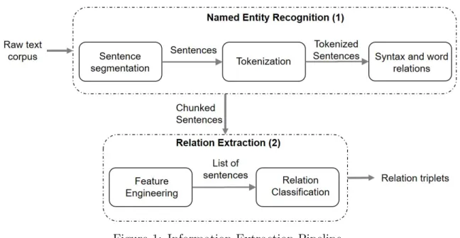
Natural Language Processing (NLP) is a specialized field in Artificial Intelligence (AI) which deals with processing and analyzing such documents automatically, with little or no human interference. Applications of NLP are found in AI assistants, language translation, and question-answering systems, for example. One specific NLP task is Information Extraction (IE), which refers to the process of extracting relevant and meaningful information based on user’s needs [4]. IE is a two-step process where

(13)

the first step comprises extracting several types of entities of interest (named entities) from the text and the second step includes identifying relations between the extracted named entities (Figure 1). Thus, the goal of IE is to convert the free text into a format that can be more readily analyzed, stored, processed or visualized.

Figure 1: Information Extraction Pipeline

Several computational methods have been proposed for both steps of the IE process, named entity recognition and relation extraction. These methods comprise rule-based approaches, shallow Machine Learning (ML) and Deep Learning techniques. Each method has its advantages and disadvantages, and their adoption varies between application domains.

1.2 Named Entity Recognition

Named entity recognition (NER) is the first step in the IE workflow (Figure 1(1)). Named entities are defined as expressions and phrases occurring in a text which can be tagged to specific categories of NUMEX, TIMEX or ENAMEX [5]. NUMEX category represents numerical expressions, such as Money and Percentage, while

(14)

categories represent proper names, such as Person, Organization and Location.

Specific application domains, require domain-specific categories of named entities. For example, the Automatic Content Extraction (ACE) program sub-divides the three basic categories into geo-political facilities, water bodies, weapons, substances and vehicles, to serve the defense domain of the Defense Advanced Research Projects Agency (DARPA) [6]. Similarly in a biomedical domain, the entities of interest are drug names, doses, and diseases treated by drugs.

Thus, NER involves the task of identifying such an entity in a natural language text and classifying it into a specific category using a series of steps. First, individual sentence boundaries are identified in the raw text using the sentence segmentation. Second, each sentence is tokenized into individual words, and stemming is performed. For example, words ‘‘indicated’’ and‘‘indication’’ in sentences are replaced by the

stem of these words‘‘indicate’’. Third, each tokenized sentence’s syntax and word

context are captured using, for example, Parts of Speech (POS) labelling, which tags each word to its syntactic part, such as, verb, noun, pronoun, adjective and conjunction. The result of this step is a list of POS tagged sentences. Finally, POS-tagged words are classified into specific named entity categories.

1.3 Relation Extraction

Relation Extraction (RE) is the second step in the IE workflow (Figure 1(2)). It identifies relevant semantic structures and connections between named entities in natural language texts. The relations to be extracted are often predefined by analysts for a specific domain. Consider, for example, the following sentence from a biomedical text,Advil can be used to treat headache, yielding the relationTreats(Advil, headache).

In this example, Advil is a drug named entity andheadache is adisease named entity

(15)

where the natural language text, What is the dosage of benadryl? yields a relation Dosage(benadryl,?). As shown in these two examples, the simplest representation of

relations is in the form of triplets: Relation(Entity1, Entity2).

1.4 Challenges in working with biomedical texts

Biomedical text is related to the domain of medicine, chemistry and biology. It includes, but is not limited to, information regarding the human clinical interactions, such as drugs and symptoms; and information on the chemical structure of proteins and genes. The most daunting challenge in biomedical information extraction is the large number of data sources, for example, medical records, drug labels and gene interactions. Different authors of these sources often have different means of conveying the same information leading to high ambiguity in parsing of information.

To promote machine readability, and easy electronic information sharing, FDA has introduced certain standards. For example, the agency requires drug sponsors to submit an important scientific summary about a drug in a document markup standard called Structured Product Labeling (SPL) [7]. SPL is a documentation standard approved by the Health Level Seven (HL7) organization [8]. HL7 administers such standards to ease digital health information storage, retrieval and exchange between different medical systems and institutions of the world.

SPL is divided into several sections, such as, indications, adverse reactions, precautions and special population use. Each section in the SPL is coded using a unique Logical Observation Identifiers Names and Codes (LOINC) [9] value. LOINC is an encoded dictionary which maps health related tests and metrics to unique identifiers, names and codes that are universally accepted by all biomedical systems.

However, these standards only govern the high-level document structure and the content within it is still freely styled by the author. Moreover, often these drug labels

(16)

(17)

CHAPTER 2 Related Work

In this chapter, an in-depth survey of existing computational methods for IE, such as, rule-based methods, shallow Machine Learning, and Deep Learning have been provided. Additionally, few existing tools for extracting information from SPL documents have also been analyzed.

2.1 Rule-based Methods

Rule-based IE is a pattern matching approach based on regular expressions and language grammar syntax. The target relation is identified by comparing each sentence in the text to predefined rules.

For example, an IS-A relationship can be identified by the following grammar rules: Y such as X; X and other Y; Y including X; Y, especially X. As an example,

the text,instruments such as piano will be matched by the above rule withX = piano, Y = instruments yielding the IS-A(piano, instruments) relation.

Rule-based methods do not scale well to relation extraction from many texts because of the large number of grammar rules that are needed. Additionally, the need for evaluating each data record against each rule increases computation time significantly [10].

2.2 Shallow Machine Learning

ML is the study of computer algorithms that improve automatically through experience [11]. Given observation data with input fields (independent variables) and a corresponding output field (dependent variable), ML algorithms can learn patterns in these data with the aim of accurately predicting the output for previously unseen input data. For example, given data on rain occurrences for each day and data about the speed of wind and sun intensity, ML can be used to predict if it is going to rain or not on any future day given wind speed and sun intensity for that day. This type of

(18)

ML problem is called a classification problem. If the application classifies the output field to any one of the two categories (for instance, Rain/No Rain or 0/1) then it is a binary classifier. If it classifies the output field to more than two categories (for instance, Summer/Winter/Fall/Spring) then it is a multi-class classifier.

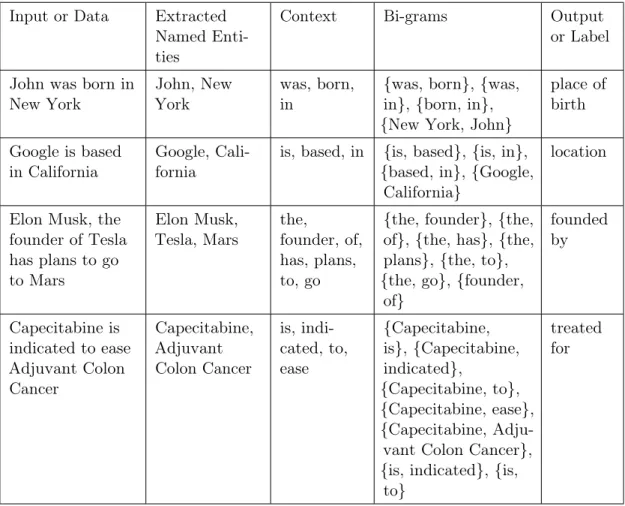
Feature engineering forms an important aspect of training an ML algorithm, and it is an active area of research. Let the input field be a sentence and the corresponding output field be the relation existing in the sentence as illustrated in Table 1. The IE pipeline will begin with the extraction of named entities in the sentence (Figure 1 and Chapter 1). The context of these named entities comprises words surrounding them, for example, words occurring in between them, and words preceding them. These words can be converted into features for an ML classifier. One of the commonly used features is bag-of-words (BOW) which is a probabilistic count of words without any syntactic or semantic knowledge about their context. POS can also be used as features and finally, more complex features could be constructed using n-grams, which is a sequence of n words (or n characters) treated as one entity (Table 1).

(19)

Table 1: Bi-gram Features for Multi-Class Shallow Machine Learning Input or Data Extracted

Named Enti-ties

Context Bi-grams Output

or Label

John was born in New York

John, New York

was, born, in

{was, born}, {was, in}, {born, in}, {New York, John}

place of birth Google is based in California Google, Cali-fornia

is, based, in {is, based}, {is, in}, {based, in}, {Google,

California}

location

Elon Musk, the founder of Tesla has plans to go to Mars Elon Musk, Tesla, Mars the, founder, of, has, plans, to, go

{the, founder}, {the, of}, {the, has}, {the, plans}, {the, to}, {the, go}, {founder,

of} founded by Capecitabine is indicated to ease Adjuvant Colon Cancer Capecitabine, Adjuvant Colon Cancer is, indi-cated, to, ease {Capecitabine, is}, {Capecitabine, indicated}, {Capecitabine, to}, {Capecitabine, ease}, {Capecitabine, Adju-vant Colon Cancer}, {is, indicated}, {is,

to}

treated for

Shallow ML techniques that are used in IE applications can be divided into three groups, namely supervised, semi-supervised and unsupervised classification algorithms. 2.2.1 Supervised Information Extraction

Supervised ML requires a labelled data set. The data set is manually mapped to relations as the target output field, also called a label. Some of the commonly used algorithms used in supervised ML are Naive Bayes, Decision tree, Support Vector Machines (SVM).

Supervised IE is often implemented using two classifiers. The first classifier takes all possible pairs of named entities in each sentence and predicts whether a relation exists between each pair or not. Thus, the first classifier is a binary classifier with

(20)

a ‘‘YES’’ or ‘‘NO’’ label. If the predicted label for the entity pair is ‘‘YES’’, then a second, multi-class classifier is used to predict the type of relation. However, if the predicted label of the first classifier is ‘‘NO’’, there is no need to use the second classifier. This two-step procedure can speed up the process of extracting relations from texts.

2.2.2 Semi-supervised Information Extraction

Semi-supervised ML uses both manually labelled and unlabelled data for train-ing. Relation Bootstrapping, Dual Iterative Pattern Relation Extraction (Dipre) are examples of semi-supervised ML.

In Relation Bootstrapping, patterns for a target relation are discovered starting from a limited number of seed patterns [12]. Lexicons refer to the vocabulary of words for a particular domain. There are many relations that can be identified between two lexicons, for example, the hyponym relation. Any lexicon which is a specialized instance of any given lexicon is called a hyponym whereas any lexicon which is a generalized instance of the given lexicon is called a hypernym. For instance, England

is the hyponym for Country which is the hypernym. Similarly, Apple is the hyponym

for the hypernym Fruit.

Relation Bootstrapping algorithm consists of the following steps [12]. 1. Define the target relationship based on the requirement and select a large text

containing instances of the target relationship.

2. Hand curate a list of pairs which follow the target relationship to serve as the seed patterns.

3. For each pair in the seed list, search sentences in the text where the pair is mentioned and record its environment, using for example, BOW as features. The environment refers to the words surrounding the seed pair.

(21)

4. Classify the environment as positive if it represents the target relationship, otherwise classify it as negative.

5. If the environment is positively classified, add the pattern to the seed list. 6. Repeat Steps 3 to 5.

The algorithm was tested to identify hyponym relations. The relation pairs were extracted from the text of Academic American Encyclopedia [13] and then compared to the WordNet lexicon [14] for evaluation. WordNet contains a hierarchical hyponym and hypernym representation of words. Out of the 152 extracted relations, 106 relations had both words of the relation pair in the WordNet lexicon, and out of these 106 relations, 61 relations were found in the WordNet hyponym hierarchy. Thus, the accuracy for the reported experiment was close to 60%. The main challenge faced by this algorithm was to identify the relations when words have different meanings based on the context of use. For instance, a sentence, ‘‘Targets, such as aircraft were identified’’ yieldshyponym(aircraft, target), while a sentence, ‘‘There are many vehicles, such as aircraft’ yields hyponym(aircraft, vehicle). A solution proposed in

the paper selected the hyponym relation which has a higher probability of occurring in the WordNet hierarchy, in this case hyponym(aircraft, vehicle).

Dual Iterative Pattern Relation Extraction (Dipre) is a second example of a semi-supervised ML technique. It was applied to extract Book(Author, Title) pair

relations from the World Wide Web (WWW) [15]. The method is based on the dual principle which states that given a set of data tuples for a given relation, it is possible to extract all patterns representing that relation. Conversely, given a set of patterns for a relation, it should be possible to extract all data tuples following that relation. A pattern is defined by the tuple, <order, urlprefix, prefix, middle, suffix>, where

(22)

• prefix refers to the m (m can be tuned) characters occurring before the Author.

• middle stands for the text occurring between the Author and theTitle.

• suffix is the m characters occurring after theTitle.

• order is a Boolean value which indicates the order in which Author andTitle

occur in the text.

• urlprefix is the longest URL prefix pattern.

Similarly, an occurrence is defined by the tuple, <Author, Title, Order, URL, Prefix, Middle, Suffix>. URL is the web page address where the given Author and Title occur while Prefix,Middle,Suffix and Order have the same meaning as that of

the pattern. The pseudo-code of Dipre is given in Appendix [15]. It was successfully applied to extract a list of 15,000 book pairs containing (Author, Title) from the WWW starting with only 5 books as the seed tuples. The main challenge for Dipre algorithm was to ensure that the newly added tuples were books and not articles. Inclusion of articles caused the algorithm to diverge from the target relation extraction. Distant Supervision is a third example of a semi-supervised ML method [16] inspired by the Relation Bootstrapping algorithm [12]. This method, also called

Snowball, was used to identify hypernym relations by automatically learning the

syntactic patterns instead of providing seed patterns.

In the given text corpora, every noun pair, which represented a hypernym relationship in the WordNet hierarchy [14] was marked as known hypernyms. Next, sentences which contained these known hypernym noun pairs were extracted from the corpora. Using the MINIPAR parser [17], these sentences were converted into their dependency tree representation depicting the grammatical relation between the words. The features from the resulting dependency trees were used to train a one-class classifier to identify hypernyms.

(23)

to Snowball. Similar to the training phase, first, MINIPAR was used to create a dependency tree of the sentence. Second, the extracted features from the dependency tree were used to classify if the noun pair present in the test sentence belonged to the hypernym relation or not. This algorithm for automatic identification of hypernym relationship was more advanced and more effective as compared to other semi-supervised methods [12, 16].

2.2.3 Unsupervised Relation Extraction

Unsupervised relation extraction is a domain independent method which extracts all frequently occurring relations without any human intervention. This method uses large amounts of unlabeled text corpora and needs no human-provided syntactic patterns or seed relation noun pairs for training. In [18], an Open IE system called text runner system is introduced. Open IE is an unsupervised technique to extract all possible relations from a given text corpus in a single iteration. The proposed system assigned a probability to the extracted relations and indexed them to facilitate their efficient extraction and user exploration.

2.3 Deep Learning

Deep Learning is a specialized form of ML. It is an artificial neural network which is inspired by the way a human brain works. The basic building block of artificial neural network is a neuron which takes multiple weighted inputs and produces outputs based on an activation function. There are multiple connected layers of such neurons passing their output as input to the next layer. Deep learning has an ability to automatically learn the important features from the raw data during the iterative training phase. The training phase involves running two steps, namely forward pass and back propagation, based on gradient descent algorithm [19]. Deep learning is a vast topic in itself and we have skipped an in-depth information about it in this thesis.

(24)

2.4 Existing Tools for Parsing SPL 2.4.1 LabeledIn

LabeledIn is an open source catalog of labeled indications for human drugs [20]. The feature that makes LabeledIn more efficient than other similar initiatives of disease-drug relationships is the fact that it involves automatic text mining and human review. The automatic process is used initially to remove redundancies and pre-compute mention of diseases in drug labels. Then the human review process involves three bio-medicine experts to go through two rounds of manual review to adjust or add new mappings as needed. Another distinguishing feature of the LabeledIn catalog is that it includes important drug-specific properties, such as ingredient, dose form, and strength, to differentiate between indications. LabeledIn catalog only focuses on 250 highly accessed drugs in PubMed [21] Health and consist of 7805 drug-disease treatment relationships.

2.4.2 Structured Product Labels eXtractor (SPL-X)

Structured Product Labels eXtractor or SPL-X [22] is a suite of Java programs that uses NLP to extract and generate critical drug-related information utilizing publicly available medical resources such as MetaMap [23]. SPL-X performs the extraction of indications using three stages - pre-processing to extract and segment ‘‘Indications’’ section from SPL labels, identifying medical concepts using MetaMap scheduler, and post-processing of MetaMap output. The extracted indications are encoded using Unified Medical Language System (UMLS) identifier [24].

Finally, SPL-X uses RxNorm drug terminology [25] to link the extracted UMLS indications to standard medical drug codes. SPL-X processed a total of 6797 drug labels and mapped around 19,473 unique drug–indication pairs.

(25)

CHAPTER 3 Materials and Methods

In this chapter, the data collection process used to prototype the solution has been described. Details on the data set creation and the method used for building and validating the classifier which can identify pediatric related text have also been provided.

3.1 Data Collection

Weekly archives of FDA approved drugs were downloaded from DailyMed [26] on August 31, 2019. The downloaded archive contained various sub-directories, one for each drug. Each drug directory comprised the SPL file and images referenced in the SPL files, such as pharmaceutical company logo, chemical structure of the drug ingredients or the image of a drug packaging. 500 drug directories were randomly sub-sampled, and the SPL file from each of these directories was copied to a single local directory to facilitate further processing.

To process each SPL file, an SPL parser in Python language was built. The lxml XML toolkit [27] was used to search and extract text segments from the SPL files. For the sake of uniformity, only those SPL files which contain Indication And Usage section identified by the LOINC 34067-9 were processed. The task to extract

pediatric related text from the SPL files was challenging because this information is not uniformly tagged in all SPL files. Therefore, an iterative extraction approach was implemented.

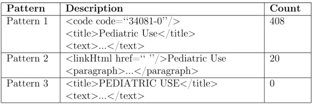
The extraction was begun by identifying paragraphs tagged with LOINC 34081-0 forPediatric Use sections (Table 2, Pattern 1). Next, randomly selected SPL files that

did not have this pattern were manually examined to construct the second pattern (Table 2, Pattern 2). Likewise, a third pattern (Table 2, Pattern 3) was constructed manually by examining SPL files which were filtered out by the first two patterns.

(26)

Case-insensitive search was used for Patterns 2 and 3.

Table 2: Patterns for Extracting Pediatric Use Section from SPL files

Pattern Description Count

Pattern 1 <code code=‘‘34081-0’’/> <title>Pediatric Use</title> <text>...</text>

408 Pattern 2 <linkHtml href=‘‘ ’’/>Pediatric Use

20 Pattern 3 <title>PEDIATRIC USE</title>

0 3.2 Data Description

Two separate data segments comprising paragraphs relevant to Pediatric Use

(positives) and paragraphs not relevant to Pediatric Use (negatives) was constructed.

To construct the positive data segments, all paragraphs matching one of the three search patterns (Table 2) were extracted from the SPL files. This comprised of paragraphs related to Pediatric Use. The negative data segments were constructed

by extracting paragraphs from four sections of the SPL files using their respective LOINCs (Table 3). Thus, it comprised of paragraphs not related to Pediatric Use.

Table 3: Other sections with associated LOINCs extracted for negative data

Section Name LOINC

Geriatric Use 34082-8

Nursing Mothers Section 34080-2

Pregnancy Section 42228-7

Lactation Section 77290-5

3.3 Data Pre-Processing

After identifying the positive and negative text segments, each segment was cleaned using the NLTK library [28] in Python (version 3.7.3). More specifically, the following pre-processing workflow was

(27)

separated by period (.) and counted the number of sentences in each of the positive and negative text segment.

2. Tokenization - Each resulting sentence was partitioned into their constituent words.

3. Removal of stop words - Commonly used words, such as, and,the,a; andis were

removed. An updated built-in NLTK Stopwords Corpus [28] which contains

2,400 stop words for 11 languages was used. Words with negative connotation, for example,no, nor and not from the English language stop words list (n=179)

were removed to cater to the problem domain and use case.

4. Lemmatization - Different forms of the same word were replaced by their base word, also called lemma. For example, words such as ‘‘indicated’’, ‘‘indicates’’

and ‘‘indication’’ were replaced by the lemma ‘‘indicate’’. More specifically, the WordNetLemmatizer package [29] in the NLTK library was used. In order to

get the most relevant syntactic lemma, WordNetLemmatizer uses four types of

POS tags, namely nouns, verbs, adjectives and adverbs. Therefore, first, POS for each word were extracted with the NLTK pos_tag() function. Second, the

extracted POS tags were used to compute the lemmas.

5. Removal of low frequency tokens - Elimination of all words which had a frequency count less than or equal to 5 was performed. This helped in removing words that do not contribute towards identifying pediatric and non-pediatric text, such as specific drug names, for example.

6. Encoding - The text data of each sentence was represented using BOW features. The Term Frequency - Inverse Document Frequency (TF-IDF) encoding with the BOW was used which converts each tokenized word to its respective occurrence

(28)

frequency in the sentence. Thus, each word is represented as a floating number between 0 and 1 giving the word’s normalized occurrence frequency. The

TfidfVectorizer library implementation available in the Scikit-Learn [30] was

used.

3.4 Data Set Labelling 3.4.1 Positive Data Set

Each pre-processed pediatric related sentence (positive data set) was labelled with ‘‘1". Each sentence corresponds to one tuple or data-row in the data set. 3.4.2 Negative Data Set

Each pre-processed non-pediatric sentence (negative data set) was labelled with ‘‘0". Each sentence corresponds to one tuple or data-row in the data set.

3.5 Baseline Models

Baseline classification models were created using simple and interpretable ML algorithms. The accuracy scores of these models were used to compare against the three validation experiments (defined later in the chapter) to evaluate the prototype solution. The data set for the baseline binary models was prepared using the following method. First, the labelled positive and negative data sets were merged and shuffled. Second, StratifiedShuffleSplit() function from Scikit-Learn [30] was used to split the

shuffled data set into two parts comprising of 66% and 34% of the data, respectively. The larger data set was used for training, while the remaining 34% was used for testing. The StratifiedShuffleSplit() function ensures that both, training and testing

data sets, contain equal distribution of positive and negative data tuples. Decision Trees, K-Nearest Neighbors (k-NN) and Support Vector Machine (SVM) were used as the baseline models.

(29)

3.5.1 Decision Trees

Decision Tree is a simple supervised ML classifier. It distinguishes between the target classes by learning simple decision rules. There are various algorithms, such as C4.5 [31], CART [32], SPRINT [33], which implement Decision Trees differently based on the tree creation method, or the type of target and feature data supported. We used the Scikit-Learn [30] library implementation of Decision Trees which uses the CART algorithm. Decision Tree is highly interpretable and easy to visualize in the form of trees.

3.5.2 k-NN

k-NN is another basic classification algorithm in ML belonging to the supervised learning domain. The k-NN algorithm is dependent on the assumption that similar data points are close to each other. To classify a data point, a specified number (k) of its closest neighbors are retrieved [34]. The majority class of the neighbors is used to classify the data point. The number of neighbors (k) is the core deciding factor for the predictive model. Although the Euclidean distance function is the commonly used distance metric in k-NN, other functions like cosine, minkowski, manhattan can also be used [35]. /the k-NN algorithm is easy to implement as it does not need any assumptions for underlying data distribution and does not need training data for model generation.

3.5.3 SVM

SVM is a supervised machine learning classifier which learns a separating hyper-plane [36]. In two dimensional space, this hyperhyper-plane corresponds to a line between the two target classes in a given data set. The tuning parameters for SVM are the kernel, regularization and gamma. Kernel defines the higher dimension where the separating hyperplane is to be computed. Regularization defines the extent of

(30)

permissible misclassification. Gamma defines to what extent the data points should be considered while computing the separating line. The Scikit-Learn [30] library implementation of SVM which uses a Sequential Minimal Optimization (SMO)-type algorithm to maximize the width of the margin [37] was used.

3.6 Experiment 1 - Cross Validation

Cross validation is a common resampling technique used to evaluate and compare ML models’ performance on unseen data [38]. It is also used for model selection. To implement cross validation, the training data set is divided into k equal parts or folds: one part is used for validation and the remaining k-1 parts are used for training the model. This process is repeated k times such that during each iteration, distinct yet slightly overlapping training samples are used to train the model. The performance of the resulting k trained models are averaged and reported. The model with high mean cross validation performance indicates that it generalizes well to unseen data.

Data Set - k = 10 was used as the preferred value to get k-fold cross validation results that generalize well to the entire data set [38]. Thus, the training data set was split into 10 equal parts. Next, two variations of k-fold cross validation over each of the 10 iterations were executed. For the first variation, 9 parts of the data for training and the remaining 1 part of the data for validating the classifier was used. For the second variation, part of the data for training and the remaining 9 parts of the data for validating the classifier was used. This gave the training metrics. I tested the classifier after each iteration of the k-fold on the 33% of the held-out data set. This gave the testing metrics. The average metrics of both training and testing were reported.

(31)

3.7 Experiment 2 - Retrospective Validation

For the ML solution, retrospective study [39] was used to evaluate the model on data which is positive, i.e. pediatric related. The fact that patterns 1, 2 and 3 can be used to extract pediatric related text has been established. In this retrospective study, I go back to the time when patterns 2 and 3 were not identified and use only the pattern 1 text as the positive training data set to build our ML model. The model is tested to evaluate if it is able to correctly predict the text containing patterns 2 and 3 as positive or not. This experiment evaluates if the model is able to generalize well to identify patterns which we had already established.

Data Set - SPL files for retrospective validation experiment were separated as follows:

For the positive training data set, Pediatric Use text from all files containing

the pattern 1 (Table 2) was selected. As before, each pre-processed sentence of the extracted paragraphs corresponds to one tuple. For the negative training data set, equal number of sentences not related to Pediatric Use (Table 3) was selected.

For the testing data set, all text from SPL files containing the patterns 2 and 3 (Table 2) was selected. Every sentence of the paragraphs containing patterns 2 and 3

is labelled as positive data. All other sentences are labelled as negative. 3.8 Experiment 3 - Prospective Validation

Prospective studies plan to classify data that has not been labelled yet [39]. The model was evaluated on unseen data which resembles actual data before deploying the model. Prospective validation was performed using the best classification model based on cross validation and retrospective validation results.

(32)

Data Set - The training and testing data sets for this experiment is same as used for the baseline models( 3.4, 3.5). The prospective validation data set used to evaluate our experiment comprised of all text from the SPL files which do not contain any of the three pediatric pattern but contain pediatric related text. To construct this data set, the following steps were used:

First, the SPL files which did not contain any of the three patterns were isolated. These either had no ‘‘Pediatric Use’’ section or were not identified using any of the

three patterns. Second, a case-insensitive regular expression search for the phrase

‘‘Pediatric Use’’ and selected the files which contained the regular expression was

performed. Third, each sentence from these files was used as the prospective validation data set tuple.

Since this is the actual data which the classifier has to classify, there is no target labels for any tuple. After classification, each tuple in the result comprised of a sentence and a corresponding predicted class of ‘‘0" or ‘‘1". The tuples classified as ‘‘1" were extracted into a csv file and used to measure the accuracy of the method by manually examining these classification results. First, a manual lookup for the

‘‘Pediatric Use’’ section in each SPL file is performed. Second, for each sentence

occurring in the section, search for a matching tuple in the csv file is done. A count of the matches is kept in order to compute results.

3.9 Performance Evaluation

Computational methods for IE are typically evaluated using the following four metrics,accuracy,precision,recall andF1. LetRbe the target relation to be extracted

from texts. The following metrics are first defined.

• True Positives (TP) are the test instances which are correctly classified as

(33)

• True Negatives (TN) are the test instances which are correctly classified as not

belonging to R by the ML classifier.

• False Positives (FP)are the test instances which belong to R but are misclassified

as not belonging to R by the ML classifier.

• False Negatives (FN) are the test instances which do not belong to R but are

misclassified as belonging to R by the ML classifier.

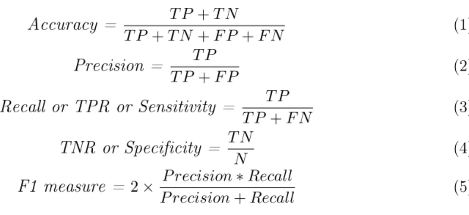
Accuracy is defined by the ratio of instances correctly classified (TP, TN) to all

the given instances (Equation 1). Often accuracy is not the optimal scoring technique for classification models because there can be an imbalance in the number of instances in each class in the training data set. In such scenarios, precision andrecall scores

can be more informative.

Precision is defined as the fraction of instances truly classified as R to the number

of all instances classified as R (Equation 2).

Recall, also called True Positive Rate (TPR) or Specificity is defined as the

fraction of instances truly classified as R to the number of instances actually belonging to R (Equation 3). It evaluates the ability of the classifier to correctly identify the positive test instances.

Another related metrics, True Negative Rate (TNR) or Sensitivity is defined as

the fraction of TN to the actual number of negative instances (N) in the data set (Equation 4). It evaluates the ability of the classifier to correctly identify the negative test instances. If there is an uneven class data set, a balance between precision and recall is needed which is measured by computing theF1 measure (Equation 5).

Support is another metrics which helps in evaluating the accuracy of the binary

classifier. It is the number of instances belonging to each class in the given test instances.

(34)

of the classifier by computing ratio of TPR to TNR. The ROC curve evaluates how well the classifier is able to separate the 2 classes of test instances. The Area Under the Curve (AUC) gives the measure of the separability in the ROC curve. If the AUC

for ROC is closer to 1, it means that the classifier is able to distinguish the classes very well while if the AUC is 0.5, it means that the classifier is not able to separate the classes at all.

Accuracy = 𝑇 𝑃 +𝑇 𝑁 𝑇 𝑃 +𝑇 𝑁+𝐹 𝑃 +𝐹 𝑁 (1) Precision = 𝑇 𝑃 𝑇 𝑃 +𝐹 𝑃 (2) Recall or TPR or Sensitivity = 𝑇 𝑃 𝑇 𝑃 +𝐹 𝑁 (3) TNR or Specificity = 𝑇 𝑁 𝑁 (4) F1 measure = 2× 𝑃 𝑟𝑒𝑐𝑖𝑠𝑖𝑜𝑛*𝑅𝑒𝑐𝑎𝑙𝑙 𝑃 𝑟𝑒𝑐𝑖𝑠𝑖𝑜𝑛+𝑅𝑒𝑐𝑎𝑙𝑙 (5) 3.10 Information Storage

For each SPL file, the extracted information as key-value pairs was stored in an intermediate JavaScript Object Notation (JSON) file [40] on the local file system where the parser was run. As depicted in Figure 2, the keys were SPLFileName, genericName, pediatricUse, isPediatricSection, and pattern. The values for these keys

correspond to the SPL file name, generic name of the drug, segment of text in the

Pediatric Use section, a value from {0, 1} signifying if this is a pediatric relevant text,

and a value from {1, 2, 3, -1} signifying the matching pattern.

(35)

CHAPTER 4 Results

In this chapter, the results of this end-to-end solution including collection of data, creation of baseline models and evaluation of the three experiments, namely cross validation, retrospective validation and prospective validation have been provided. 4.1 Data Collection

From the downloaded 40,525 SPL files, 500 files are randomly subsampled. 5 SPL files which did not contain Indication And Usage section were identified and

filtered making the total number of files to be 495. Using the three patterns described in Section 3.1, the Pediatric UseSection from these 495 SPL files (Table 4) was then

extracted.

Table 4: Data Collection forPediatric Use Section from SPL files

Pattern No. of SPL files Pattern 1 408

Pattern 2 20

The remaining 67 SPL files either do not contain pediatric related text or is not identified by the three patterns. Using the case in-sensitive regular expression search as described in 3.7, 33 files which contained pediatric related text but none of the three patterns were separated. The remaining 34 files did not contain any pediatric related text.

4.2 Data Pre-Processing

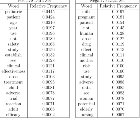
After applying sentence segmentation and tokenization on the positive and negative data set, 4751 unique words were reported. Table 5 illustrates the relative frequencies of the top 20 occurring words in positive and negative data sets. As the intuition suggests, for positive data set, words such as pediatric, child and age

(36)

that contains text corresponding to ‘‘Geriatric Use’’, ‘‘Nursing Mothers Section’’, ‘‘Pregnancy Section’’ and ‘‘Lactation Section’’, words such as pregnant, mother and

elderly are some of the most frequently occurring words.

Table 5: Most Frequently Occurring Words Positive Data Set

Word Relative Frequency

pediatric 0.0445 patient 0.0424 age 0.0210 year 0.0197 use 0.0196 not 0.0189 safety 0.0168 study 0.0156 establish 0.0132 see 0.0128 clinical 0.0121 effectiveness 0.0117 dose 0.0103 treatment 0.0095 child 0.0081 adverse 0.0078 trial 0.0077 reaction 0.0071 adult 0.0068 efficacy 0.0062

Negative Data Set Word Relative Frequency

milk 0.0197 pregnant 0.0181 patient 0.0154 not 0.0145 human 0.0128 dose 0.0122 drug 0.0119 effect 0.0113 clinical 0.0111 mother 0.0110 risk 0.0100 use 0.0100 study 0.0095 adverse 0.0088 data 0.0085 see 0.0083 woman 0.0078 potential 0.0071 elderly 0.0070 nursing 0.0067 4.3 Data Analysis

The word count per sentence of positive and negative data set after the data pre-processing step defined in 3.3 was analyzed. As shown in the Figure 3, the dashed line plot corresponds to the negative text, i.e. text from other 4 sections and text from files not containing Pediatric Use section. Similarly, the solid line plot corresponds

to the positive text, i.e. text from all Pediatric Use. The weighted average based on

all the word count frequencies for positive data turns out to be 7.5 and for negative data turns out to be 6.7. The short length sentences were padded to make a constant

(37)

length data set.

Figure 3: Word count per sentence

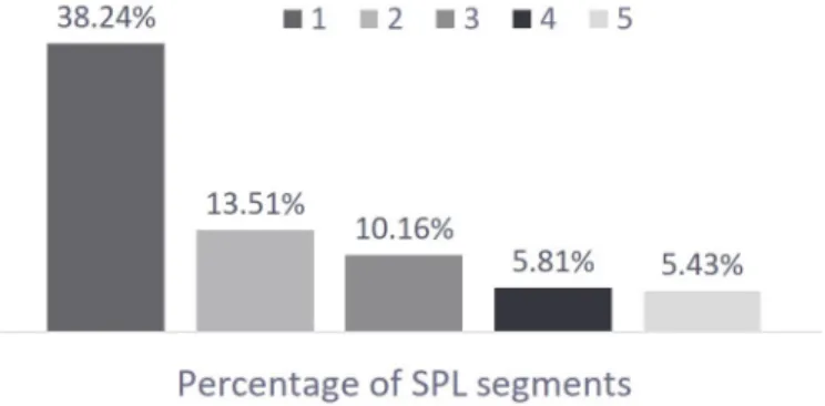
Additionally, the pediatric related text segments were also analyzed to count the number of sentences in each segment. As indicated by the Figure 4, majority (38.24%) of pediatric related text segments comprised of one sentence only. Thus, individual sentences were considered as tuples in the data sets resulting in 8492 pre-processed negative data tuples and 2480 pre-processed positive data tuples. In order to balance the data sets, 2480 negative tuples were randomly subsampled.

Figure 4: Top 5 sentence counts in Pediatric related text segments 4.4 Feature selection and encoding

TfidfVectorizer was used to encode the sentences into features. 1503 number of features corresponding to the word vocabulary of the positive and negative data set

(38)

combined were extracted. In order to identify the most useful features from these 1503 features, feature selection was performed. The Chi square [41] statistic between each feature and the expected class was used for feature selection. Chi square test provides the significance of observed values (features in our case), relative to the expected values (class in our case). It measures the correlation between different features. Thus, features which are more correlated to the output class as compared to the features which are independent of the output class and are therefore irrelevant were identified. More specifically, the chi2 statistics and the SelectKBest routine of the Scikit-Learn

were used to select the k most relevant features. The value of k was tuned using the

baseline models and was fixed to 200 for the subsequent three tests. 4.5 Baseline Classifier Validation

In order to identify the best parameters for the baseline models, grid search which does an exhaustive search over the given parameter values was used. Grid search using 20 folds with a Stratified K-Fold cross validation was implemented. The optimal values that were returned in the result were used to train the baseline models. Thus, for Decision Tree, criteria = entropy was used for learning. For SVM, gamma = 0.005 and regularization = 4 was used. 4 models based on the 4 kernel functions of

SVM, named linear, poly, rbf and sigmoid were trained. For k-NN, the minkowski distance (and p = 7) as the function to compute the distance between neighborhood

points and the number of neighbors k = 5(Figure A.6) was used.

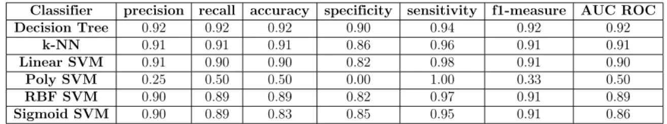
Based on the performance metrics (Table 6), Decision Tree, k-NN and Linear SVM have high precision, recall and AUC ROC values. This signifies that these models are able to distinguish between pediatric related and non-pediatric related text with 90 % accuracy provided that the non-pediatric text is from one of the other 4 sections (Table 3). A sample text which was neither pediatric related nor from one

(39)

of the other 4 sections was considered. Each of the top three high accuracy models, falsely classified it as positive. This result provided an intuition that the negative training data set is not representative of the actual data on which these models are to be used.

Table 6: Performance of baseline classifiers.

Classifier precision recall accuracy specificity sensitivity f1-measure AUC ROC

Decision Tree 0.92 0.92 0.92 0.90 0.94 0.92 0.92 k-NN 0.91 0.91 0.91 0.86 0.96 0.91 0.91 Linear SVM 0.91 0.90 0.90 0.82 0.98 0.91 0.90 Poly SVM 0.25 0.50 0.50 0.00 1.00 0.33 0.50 RBF SVM 0.90 0.89 0.89 0.82 0.97 0.91 0.89 Sigmoid SVM 0.90 0.89 0.83 0.85 0.95 0.91 0.86

In order to test this intuition, the models were re-trained by including the text from the 34 files which did not contain any pediatric related text( 4.1). As expected, the resulting models correctly classified the sample text while preserving similar values of the performance metrics(Table 7).

Table 7: Performance of baseline classifiers with additional negative data Classifier precision recall accuracy specificity sensitivity f1-measure AUC ROC

Decision Tree 0.92 0.92 0.92 0.93 0.91 0.92 0.91

k-NN 0.89 0.89 0.89 0.90 0.88 0.89 0.89

Linear SVM 0.89 0.89 0.90 0.93 0.86 0.89 0.90

4.6 Experiment 1 - Cross Validation

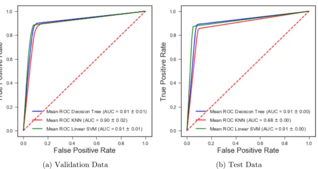
K-fold cross validation with k = 10 was implemented on the top three baseline classifiers, i.e. Decision Tree, k-NN and Linear SVM. For the first variation of cross validation, 9 parts of the split data was used for training and 1 part for validation. Tables 8 and 9 summarize the mean training and mean testing accuracy metrics respectively. Figure 5 provides the comparative ROC curve for training and testing. The results of the second variation of k-fold cross validation (1 part for training and 9 parts for validation) have been omitted due to low accuracy.

(40)

Table 8: Cross Validation 9 parts train, 1 part validation results - Training Accuracy Classifier precision recall accuracy specificity sensitivity f1-measure AUC ROC Decision Tree 0.91±_{0.01 0.91}±_{0.01 0.91}±_{0.01 0.92}±_{0.00 0.90}±_0.02 _0.91±_0.01 _0.91±_0.01

k-NN 0.90±_{0.02 0.90}±_{0.02 0.90}±_{0.02 0.90}±_{0.04 0.89}±_0.01 _0.90±_0.02 _0.90±_0.02 Linear SVM 0.91±_{0.01 0.91}±_{0.01 0.91}±_{0.01 0.94}±_{0.02 0.88}±_0.02 _0.91±_0.01 _0.91±_0.01

Table 9: Cross Validation 9 parts train, 1 part validation results - Testing Accuracy Classifier precision recall accuracy specificity sensitivity f1-measure AUC ROC Decision Tree 0.91±0.00 0.91±0.00 0.91±0.00 0.93±0.01 0.89±0.01 0.91±0.00 0.91±0.00

k-NN 0.88±0.01 0.88±0.01 0.88±0.01 0.91±0.02 0.85±0.04 0.88±0.01 0.88±0.00 Linear SVM 0.92±0.01 0.91±0.00 0.91±0.00 0.95±0.02 0.87±0.02 0.91±0.00 0.91±0.00

(a) Validation Data (b) Test Data

Figure 5: K-fold Cross Validation ROC curve with 9 parts train, 1 part validation The results show that taking into consideration the mean metrics and their standard deviations, the precision, recall and f1-measure of all the three classifiers are similar. The classifiers are able to distinguish between pediatric and non-pediatric text with 90% accuracy for training and testing data sets. Therefore, none of the three classifiers were discarded yet.

(41)

4.7 Experiment 2 - Retrospective Validation

Retrospective validation was implemented on the top three baseline classifiers. The results of the retrospective experiment are summarized in table 10. The success of this experiment is defined by how well the classifiers correctly predict the label for the positive test data, i.e. the pediatric related data. Out of the three classifiers, the TPR of k-NN is reported as the highest suggesting that k-NN is able to correctly identify 97% of pediatric text. Low TPR of Linear SVM indicates that the target classes are not linearly separable by a line. Using the retrospective and the cross validation results, k-NN was selected as the model of choice for the next experiment.

Table 10: Retrospective Validation Results

Classifier TPR

Decision Tree 0.9379

k-NN 0.9724

Linear SVM 0.9172 4.8 Experiment 3 - Prospective Validation

Considering each sentence as a tuple, 6233 tuples were extracted after data pre-processing of the 33 SPL files which did not contain any pediatric pattern( 4.1). k-NN was used to predict the classification for each of the 6233 tuples. 3123 tuples were identified as ‘‘1" or pediatric related. To evaluate the results, a manual inspection as discussed in 3.8 was performed. It was discovered that all the ‘‘Pediatric Use" text from the 33 SPL files were correctly classified as ‘‘1" in the csv file. Using 10% of the validation data to compute the confusion matrix, the Table11 is reported. The results show that the TP is high but at the same time FP is significant.

(42)

Table 11: Confusion Matrix for 10% sampled validation data

Predictive Values

Class 0

Class 1

Actual Values Class 0 TN =

_{Class 1}

_{FN =}

70 ₆

_{TP =}

FP =

12 ₇₆

(43)

CHAPTER 5

Conclusion and Future Work 5.1 Conclusion

In this exploratory project, Natural Language Processing and Machine Learning techniques have been utilized to implement an Information Extraction system for biomedical text using Python. 500 drug labels from DailyMed [26] were processed and a classifier to identify and extract text from the pediatric use section of the drug labels was built. Review of the results indicated that the prototype has a recall of 0.93 and precision of 0.86. This shows the effectiveness of machine learning algorithms in classifying and extracting relevant information from biomedical text.

5.2 Future Work

The results of this solution indicate that there is a possibility of using ML techniques to identify pediatric related text from the unstructured drug labels. Since the resulting classification from the solution is high in TP and also in FP, a secondary classifier trained only on non-pediatric text can be implemented. This would help filter out the non-pediatric text from the results.

The pediatric text extracted from this solution can be used as the data set to identify whether the drug is safe and effective in pediatric population. The results from this evaluation can then be plugged into the data source of PediatricDB [3]. In this way, the solution can be used to extend the pediatric research work.

In the solution, each sentence is mapped to 1 tuple. A sliding window technique to group 2 or more sentences to form a tuple can also be used. Additionally, Deep Learning with word vectors (word2vec) to augment automatic feature discovery for natural language processing can be implemented.

(44)

LIST OF REFERENCES

[1] ‘‘Fact sheet: Fda at a glance,’’ https://www.fda.gov/about-fda/fda-basics/fact-sheet-fda-glance, (Accessed on 11/22/2019).

[2] A. Ferro, ‘‘Paediatric prescribing: why children are not small adults,’’British journal of clinical pharmacology, vol. 79, no. 3, pp. 351--353, Mar 2015.

[3] S. Deshmukh and N. Khuri, ‘‘Pediatricdb: Data analytics platform for pediatric healthcare,’’ in 2018 Thirteenth International Conference on Digital Information Management (ICDIM), Sep. 2018, pp. 216--221.

[4] ‘‘National institute of standards and technology: Saic information extrac-tion,’’ https://www.itl.nist.gov/iaui/894.02/related_projects/muc/index.html, (Accessed on 2/14/2019).

[5] N. Chinchor and P. Robinson, ‘‘Appendix e: Muc-7 named entity task definition (version 3.5),’’ in Seventh Message Understanding Conference (MUC-7): Proceedings of a Conference Held in Fairfax, Virginia, April 29 - May 1, 1998, 1998. [Online]. Available: https://www.aclweb.org/anthology/M98-1028

[6] S. Strassel, A. Mitchell, and S. Huang, ‘‘Multilingual resources for entity extraction,’’ in Proceedings of the ACL 2003 Workshop on Multilingual and Mixed-language Named Entity Recognition - Volume 15, ser. MultiNER ’03.

Stroudsburg, PA, USA: Association for Computational Linguistics, 2003, pp. 49--56. [Online]. Available: https://doi.org/10.3115/1119384.1119391

[7] ‘‘Structured product labeling,’’ https://open.fda.gov/data/spl/, (Accessed on 3/15/2019).

[8] ‘‘Hl7 standards,’’ http://www.hl7.org/, (Accessed on 3/14/2019).

[9] ‘‘Loinc,’’ https://www.fda.gov/ForIndustry/DataStandards/ StructuredProductLabeling/ucm162057.htm/, (Accessed on 2/22/2019).

[10] F. Reiss, S. Raghavan, R. Krishnamurthy, H. Zhu, and S. Vaithyanathan, ‘‘An algebraic approach to rule-based information extraction,’’ in 2008 IEEE 24th International Conference on Data Engineering, April 2008, pp. 933--942.

[11] T. Mitchell, Machine Learning. McGraw Hill, 1997.

[12] M. A. Hearst, ‘‘Automatic acquisition of hyponyms from large text corpora,’’ in

Proceedings of the 14th Conference on Computational Linguistics - Volume 2, ser.

COLING ’92. Stroudsburg, PA, USA: Association for Computational Linguistics, 1992, pp. 539--545. [Online]. Available: https://doi.org/10.3115/992133.992154

(45)

[13] ‘‘Academic american encyclopedia,’’ Danbury, Connecticut, USA, 1990.

[14] ‘‘About wordnet.’’ https://wordnet.princeton.edu/, 2010, (Accessed on 4/1/2019). [15] S. Brin, ‘‘Extracting patterns and relations from the world wide web,’’ in

Selected Papers from the International Workshop on The World Wide Web and Databases, ser. WebDB ’98. London, UK, UK: Springer-Verlag, 1999, pp.

172--183. [Online]. Available: http://dl.acm.org/citation.cfm?id=646543.696220 [16] R. Snow, D. Jurafsky, and A. Y. Ng, ‘‘Learning syntactic patterns for automatic hypernym discovery,’’ in Proceedings of the 17th International Conference on Neural Information Processing Systems, ser. NIPS’04. Cambridge, MA,

USA: MIT Press, 2004, pp. 1297--1304. [Online]. Available: http: //dl.acm.org/citation.cfm?id=2976040.2976203

[17] ‘‘Minipar,’’ https://gate.ac.uk/releases/gate-7.0-build4195-ALL/doc/tao/ splitch17.html/, (Accessed on 3/15/2019).

[18] M. Banko, M. J. Cafarella, S. Soderland, M. Broadhead, and O. Etzioni, ‘‘Open information extraction from the web,’’ in Proceedings of the 20th International Joint Conference on Artifical Intelligence, ser. IJCAI’07. San Francisco, CA,

USA: Morgan Kaufmann Publishers Inc., 2007, pp. 2670--2676. [Online]. Available: http://dl.acm.org/citation.cfm?id=1625275.1625705

[19] S. Ruder, ‘‘An overview of gradient descent optimization algorithms,’’ CoRR,

vol. abs/1609.04747, 2016. [Online]. Available: http://arxiv.org/abs/1609.04747 [20] R. Khare, J. Li, and Z. Lu, ‘‘LabeledIn: cataloging labeled indications for human

drugs,’’ J Biomed Inform, vol. 52, pp. 448--456, Dec 2014.

[21] ‘‘Pubmed,’’ https://www.ncbi.nlm.nih.gov/pubmed/, (Accessed on 11/22/2019). [22] K. W. Fung, C. S. Jao, and D. Demner-Fushman, ‘‘Extracting drug indication

information from structured product labels using natural language processing,’’

Journal of the American Medical Informatics Association : JAMIA, vol. 20, no. 3,

pp. 482--488, May 2013.

[23] A. R. Aronson and F.-M. Lang, ‘‘An overview of metamap: historical perspective and recent advances,’’ Journal of the American Medical Informatics Association : JAMIA, vol. 17, no. 3, pp. 229--236, 2010.

[24] O. Bodenreider, ‘‘The unified medical language system (umls): integrating biomed-ical terminology,’’ Nucleic acids research, vol. 32, no. Database issue, pp.

(46)

[25] S. Liu, Wei Ma, R. Moore, V. Ganesan, and S. Nelson, ‘‘Rxnorm: prescription for electronic drug information exchange,’’ IT Professional, vol. 7, no. 5, pp. 17--23,

Sep. 2005.

[26] ‘‘Dailymed,’’ https://dailymed.nlm.nih.gov/dailymed/, (Accessed on 2/17/2019). [27] ‘‘Dailymed,’’ https://lxml.de/, (Accessed on 2/18/2019).

[28] S. Bird, E. Klein, and E. Loper, Natural language processing with Python : [analyzing text with the natural language toolkit], 1st ed. O’Reilly, 2009.

[29] ‘‘Morphy - discussion of wordnet’s morphological processing,’’ https://wordnet. princeton.edu/documentation/morphy7wn, (Accessed on 4/18/2019).

[30] ‘‘Scikit-learn,’’ https://scikit-learn.org/, (Accessed on 4/19/2019).

[31] J. R. Quinlan,C4.5: Programs for Machine Learning. San Francisco, CA, USA:

Morgan Kaufmann Publishers Inc., 1993.

[32] B. Everitt, Classification and Regression Trees. Chapman & Hall, 10 2005.

[33] J. Shafer, R. Agrawal, and M. Mehta, ‘‘Sprint: A scalable parallel classifier for data mining,’’ VLDB, 08 2000.

[34] T. Cover and P. Hart, ‘‘Nearest neighbor pattern classification,’’ IEEE Trans. Inf. Theor., vol. 13, no. 1, pp. 21--27, Sept. 2006. [Online]. Available:

https://doi.org/10.1109/TIT.1967.1053964

[35] L.-Y. Hu, M.-W. Huang, S.-W. Ke, and C.-F. Tsai, ‘‘The distance function effect on k-nearest neighbor classification for medical datasets,’’

SpringerPlus, vol. 5, no. 1, pp. 1304--1304, Aug 2016. [Online]. Available:

https://www.ncbi.nlm.nih.gov/pubmed/27547678

[36] C.-C. Chang and C.-J. Lin, ‘‘Libsvm: A library for support vector machines,’’

ACM Trans. Intell. Syst. Technol., vol. 2, no. 3, pp. 27:1--27:27, May 2011.

[Online]. Available: http://doi.acm.org/10.1145/1961189.1961199

[37] R.-E. Fan, P.-H. Chen, and C.-J. Lin, ‘‘Working set selection using second order information for training support vector machines,’’ J. Mach. Learn. Res., vol. 6, pp. 1889--1918, Dec. 2005. [Online]. Available:

http://dl.acm.org/citation.cfm?id=1046920.1194907

[38] P. Refaeilzadeh, L. Tang, and H. Liu, ‘‘Cross-validation,’’ Encyclopedia of Database Systems, pp. 532--538, 01 2009.

[39] ‘‘Prospective and retrospective cohort studies,’’ http://sphweb.bumc.bu.edu/ otlt/MPH-Modules/EP/EP713_AnalyticOverview/EP713_AnalyticOverview3. html, (Accessed on 11/23/2019).

(47)

[40] ‘‘Introducing json,’’ https://www.json.org/, (Accessed on 2/22/2019).

[41] M. L. McHugh, ‘‘The chi-square test of independence,’’ Biochemia medica,

vol. 23, no. 2, pp. 143--149, 2013, pMC3900058[pmcid]. [Online]. Available: https://www.ncbi.nlm.nih.gov/pubmed/23894860

(48)

APPENDIX A A.1 k-NN Distance function analysis

Figure A.6: k-NN: Comparative analysis of accuracy with number of neighbors and distance metric

(49)

APPENDIX B B.1 Glossary

FDA Food and Drug Administration. NLP Natural Language Processing. AI Artificial Intelligence.

IE Information Extraction. NER Named entity recognition. ACE Automatic Content Extraction.

DARPA Defense Advanced Research Projects Agency. POS Parts of Speech.