PARALLEL MARKOV CHAIN MONTE CARLO METHODS FOR LARGE SCALE STATISTICAL INVERSE PROBLEMS
A Dissertation by
KAINAN WANG
Submitted to the Office of Graduate and Professional Studies of Texas A&M University
in partial fulfillment of the requirements for the degree of DOCTOR OF PHILOSOPHY
Chair of Committee, Wolfgang Bangerth Committee Members, Jean-Luc Guermond
Yalchin Efendiev Helmut Katzgraber Head of Department, Emil Straube
May 2014
Major Subject: Mathematics
ABSTRACT
The Bayesian method has proven to be a powerful way of modeling inverse prob-lems. The solution to Bayesian inverse problems is the posterior distribution of esti-mated parameters which can provide not only estimates for the inferred parameters but also the uncertainty of these estimations. Markov chain Monte Carlo (MCMC) is a useful technique to sample the posterior distribution and information can be extracted from the sampled ensemble. However, MCMC is very expensive to com-pute, especially in inverse problems where the underlying forward problems involve solving differential equations. Even worse, MCMC is difficult to parallelize due to its sequential nature—that is, under the current framework, we can barely accelerate MCMC with parallel computing.
We develop a new framework of parallel MCMC algorithms—the Markov chain preconditioned Monte Carlo (MCPMC) method—for sampling Bayesian inverse prob-lems. With the help of a fast auxiliary MCMC chain running on computationally cheaper approximate models, which serves as a stochastic preconditioner to the tar-get distribution, the sampler randomly selects candidates from the preconditioning chain for further processing on the accurate model. As this accurate model pro-cessing can be executed in parallel, the algorithm is suitable for parallel systems. We implement it using a modified master-slave architecture, analyze its potential to accelerate sampling and apply it to three examples. A two dimensional Gaus-sian mixture example shows that the new sampler can bring statistical efficiency in addition to increasing sampling speed. Through a 2D inverse problem with an el-liptic equation as the forward model, we demonstrate the use of an enhanced error model to build the preconditioner. With a 3D optical tomography problem we use
adaptive finite element methods to build the approximate model. In both examples, the MCPMC successfully samples the posterior distributions with multiple proces-sors, demonstrating efficient speedups comparing to traditional MCMC algorithms. In addition, the 3D optical tomography example shows the feasibility of applying MCPMC towards real world, large scale, statistical inverse problems.
ACKNOWLEDGEMENTS
First and foremost, I would like to thank my advisor professor Wolfgang Bangerth who has been guiding me in every aspect of research. He has also impacted me in my attitudes towards work, life and family.
I would like to express my thanks to professor Jean-Luc Guermond, professor Yalchin Efendiev and professor Helmut Katzgraber for kindly serving on my com-mittee. I thank them for the directions and comments that help shape my doctoral research.
I am grateful to the whole Bangerth research group. Especially, I would like to thank Dr. Timo Heister and Dr. Bruno Turcksin for their help on understanding parallel computing and programming in general.
Last but not least, I am thankful to my family. The support from my parents and my parents-in-law allows me to concentrate on this research. I want to thank my wife Wei who has not much to do with mathematics but with every other aspect of my life. It is her understanding and unconditional support that make this dissertation come into existence. I owe everything to her.
Part of the work presented herein was supported by the National Science Foun-dation through Award No. OCI-1148116; and by Award No. KUS-C1-016-04, made by King Abdullah University of Science and Technology (KAUST).
TABLE OF CONTENTS
Page
ABSTRACT . . . ii
ACKNOWLEDGEMENTS . . . iv
TABLE OF CONTENTS . . . v
LIST OF FIGURES . . . vii
LIST OF TABLES . . . x
1. INTRODUCTION . . . 1
1.1 Inverse problems . . . 1
1.2 Deterministic methods . . . 2
1.3 Bayesian inverse problems . . . 6
1.4 Introduction to parallel computing . . . 9
2. SOME EXISTING SAMPLING METHODS . . . 12
2.1 Importance sampling methods . . . 13
2.2 Markov chain Monte Carlo methods . . . 15
2.2.1 Markov chain and its basic properties . . . 16
2.2.2 Metropolis-Hastings algorithm . . . 18
2.2.3 Adaptive proposal for Metropolis-Hastings . . . 22
2.2.4 Diagnostic tests for MCMC algorithms . . . 24
2.3 Existing parallel MCMC algorithms . . . 29
2.3.1 Prefetching MCMC algorithm . . . 30
2.3.2 Parallel tempering method . . . 32
3. THE MARKOV CHAIN PRECONDITIONED MONTE CARLO METHOD 37 3.1 The MCPMC algorithm . . . 37
3.2 Implementing MCPMC for multiple processors . . . 42
3.2.1 Discussion on the parallel efficiency . . . 43
3.3 Example: A two dimensional Gaussian distribution . . . 47
4. APPLICATION: AN INVERSE PROBLEM WITH ELLIPTIC EQUATIONS 56
4.1 Problem description . . . 56
4.2 Enhanced error model . . . 62
4.3 Numerical results . . . 65
5. APPLICATION: THREE DIMENSIONAL OPTICAL TOMOGRAPHY . 71 5.1 The forward model . . . 73
5.1.1 The radiative transfer equation and the diffusion approximation 73 5.1.2 Fluorescence enhanced optical tomography . . . 77
5.2 The Bayesian model of the inverse problem . . . 78
5.3 Deterministic inversion and adaptive mesh refinement . . . 79
5.3.1 Deterministic inversion . . . 80
5.3.2 Adaptive mesh refinement . . . 84
5.4 Stochastic inversion using MCPMC . . . 84
6. CONCLUSIONS . . . 96
REFERENCES . . . 99
APPENDIX A. REVERSIBLE JUMP MARKOV CHAIN MONTE CARLO METHOD . . . 106
LIST OF FIGURES
FIGURE Page
1.1 A graphic illustration of a typical distributed memory cluster. . . 11 2.1 Auto-correlation function for one of the 64 estimated parameters.
Judging from this plot, we may need to use a “thinning” of 10,000 samples, that is, picking every 10,000th sample in the sequence to compute any estimate. . . 21 2.2 An illustration of the burn-in period during sampling. In this example,
the true value of the parameter is 1. It is advised to discard the first 104 samples to have a more accurate mean estimator. But this means we have to abandon 1/3 of the total computing effort. . . 21 2.3 One single iteration of the prefetching MCMC with 7 processors. . . . 31 2.4 Theoretical speedups and efficiencies of the prefetching algorithm for
different number of processors. Since in the inverse problems the com-puting time dominates the communication time, these theoretical es-timates should be close to the data from numerical experiments. . . . 33 2.5 A sequence of (unnormalized) tempered density functions for a mixed
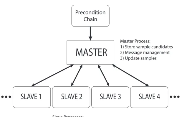
Gaussian distributions. . . 35 3.1 A graphical illustration of the modified master-slave architecture with
which we implement the MCPMC algorithm. . . 44 3.2 An illustration of the two dimensional Gaussian distribution problem
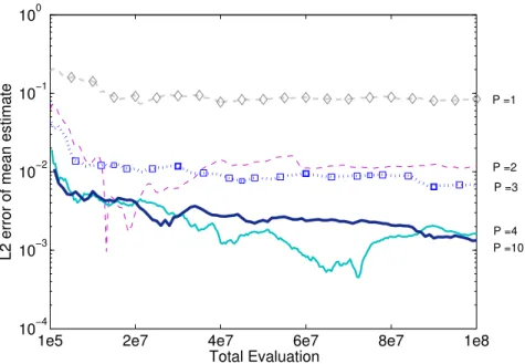
where we try to sample the distribution centered at (5,0) using a MCPMC with the preconditioning chain being an MCMC sampling the “approximate” distribution centered at (0,0). . . 48 3.3 Convergence comparison of samplers with different perturbation steps.
The x-axis is the total number of perturbation evaluations taken on the accurate model. So, for the sampler with P = 10, the total num-ber of samples shown in this plot is 107 because obtaining each sample requires running a short chain of 10 steps. On the contrary, the sam-pler withP = 1 has 108 samples shown in the plot. Even so, samplers with more perturbations demonstrate a better convergence. . . 51
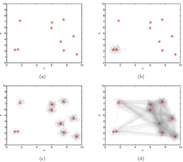
3.4 Sampling the two dimensional Gaussian mixture distribution: (a) shows the centers of the ten modes; (b) shows the result of 1000 sam-ples from an MH sampler; (c) shows the result from the MCPMC with 6 chains and 1000 samples on the sixth chain; (d) shows the sample paths for the same samples as in (c). . . 54 3.5 1000 samples from the first chain to the sixth chain of the MCPMC
al-gorithm. The temperature decreases with respect to i, i= 1,2,· · · ,6. The i-th chain serves as a preconditioner for the i+ 1-th chain which fetches samples from the preconditioner and filter samples according to its own probability distribution. . . 55 4.1 Generation of the synthetic data. The top left figure shows the
ref-erence coefficient field x(z), the top right figure shows the solution
p(z) using the reference coefficient and the bottom figure shows the adaptively refined mesh for obtaining the solution. . . 57 4.2 Four samples from a total variation prior distribution. Pixel values
vary across the range of parameters and the pictures are blocky. . . . 59 4.3 Four samples from a Gaussian prior distribution. Pixel values are
independent of the values of their neighbor. . . 60 4.4 The meshes used for the approximate model (left) and the accurate
model (right). . . 62 4.5 Error comparison for a plain MCMC algorithm with either a coarse
grid model or an EEM using one million samples. The x-axis is the 64 pixels, i.e., the components xi of the parameter which appears as a coefficient in the elliptic equation. The y-axis is the error |x¯i−x∗i|2, i.e., the square error between the mean estimator and the real value. . 65 4.6 Using the same data as above, the figure shows a comparison of the
histogram approximated density functions for the marginal distribu-tion of three coordinates: x5,x34 andx51 between the coarse grid, the fine grid and the enhanced error models. . . 66 4.7 Left: Conditional mean reconstruction using 106 samples from the
MH sampler on the fine grid. Right: Conditional mean reconstruc-tion using 106 samples from the MCPMC chain that evaluates on the accurate model. . . 69 4.8 Sampling error as defined in (4.3) for the coarse level MCMC (green),
4.9 Sampling error plotted as a function of estimated running time for the coarse level MCMC (green), fine level MCMC (blue) and MCPMC (red). 70 5.1 Left: Mesh that is used for generating the synthetic data. Right:
Diffractive excitation light that illuminates the tissue. . . 86 5.2 Meshes used in the MCPMC sampling: the top left figure shows the
parameter field discretization, the top right figure shows the coarse grid for state variables and the bottom figure shows the fine grid for state variables. . . 87 5.3 A cross section of the object showing the conditional mean (CM)
esti-mates with coarse chain MH, fine chain MH and MCPMC sampling, also in comparison with the MAP estimate computed from the deter-ministic inversion. . . 89 5.4 Comparison of the range of cells whose standard deviation is above a
certain threshold (0.00125). Left: Standard deviation using samples from the MH sampler on the fine grid. Right: Standard deviation using samples from the MCPMC sampler. . . 90 5.5 Comparison of histograms at pixels which have estimated magnitude
greater than 60% of the maximal magnitude—these are considered as the target pixels. The histogram from MCPMC is plotted in blue and that from the fine MH is plotted in red. . . 92 5.6 Autocorrelation function of randomly selected parameter components
plotted for autocorrelation time up to 3000. In each plot, the red curve is for the fine MH sampler, green for the coarse MH sampler and blue for the MCPMC sampler. . . 95 A.1 Upscaled results for a sample well log: the left two plots are the
his-togram of the boundary locations and the estimated upscaling with a fixed number of layers; the right two plots are the histogram of the boundary locations and the estimated upscaling with variable num-ber of layers and reversible jump MCMC. In the upscaled comparison plots, the wiggly solid line is the true well log, and the smoother lines are the mean, 10% and 90% upscaled estimates as indicated in the plot. Plot obtained from [21]. . . 110
LIST OF TABLES
TABLE Page
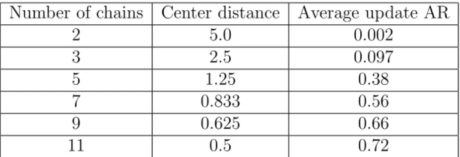
3.1 Average acceptance ratios (AR) in the update stage when using dif-ferent numbers of chains. The “center distance” column shows the distance between mean vectors of neighboring distributions. . . 49 5.1 Comparison of conditional mean (CM) and standard deviation
(std-dev) estimation between MCPMC and fine MH samplers at pixels which have estimated magnitude greater than 60% of the maximal magnitude—these are considered as the target pixels. We also com-pute a relative error defined as (meanMCPMC−meanfine-MH)
/stddevfine-MH, i.e., we compute the difference between the mean es-timates from both samplers normalized by the standard deviation of the fine MH sampler. . . 93 5.2 The integrated autocorrelation time (IACT) and the mean square
jump (MSJ) computed for several components of the parameter vec-tor. In the table, fine MH is abbreviated as “f” and MCPMC is abbreviated as “m”. . . 94
1. INTRODUCTION
1.1 Inverse problems
Much of the motivation in applied mathematics stems from the desire to under-stand the behavior of systems or to make predictions in different situations. We derive mathematical models—mostly in the form of equations—to achieve this pur-pose. A mathematical model is usually a general description that arises from our understanding of a system. For example, Hooke’s law expresses that the force that stretches or compresses a spring to a certain distance is proportional to that distance. However, for such a model to be of use, we have to understand quantitatively the “parameters” that are underlying each system. In the example of springs, different springs could have different ratios of proportion between the force and the displace-ment and it is imperative to “measure” that ratio so that we can use Hooke’s law to predict the forces. In general, we use the term “parameter” to indicate any system configuration that affects the system’s behavior. Some usual examples of parameters include equation coefficients (as in the previous example), source terms or boundary conditions.
The mathematical field of inverse problems studies mathematical techniques to infer such parameters in a model. One of the goals for the inference is to estimate the parameters so that predictions produced by such a configured model coincide with data from physical measurements. With these parameters we will be able to predict the data in the future by simulating the configured model. Another goal is to quantify uncertainties of the inference. It has been well understood that uncertainties lie in every place of the modeling process: the measurements could have errors, the
computer codes may not be completely precise due to the limitations in floating point precision, storage or computing time. Therefore, we have to address the question of how much risk there is to use the configured model.
Inverse problems have wide applications in biomedical imaging and geophysical exploration methods where direct examination of the body interior is infeasible. For example, optical tomography methods [1, 8] use light pattern observations through a body tissue to infer absorption and scattering coefficients in a mathematical model that describes photon movements. These coefficients in turn express the variations inside the tissue and can help detect, for example, the existence of a tumor. Another example are subsurface modeling/characterization of oil reservoirs and aquifers. In these problems, people are often interested in estimating the permeability field—a measure of the ability of a porous medium to allow fluids to pass through it. Since the permeability varies throughout the entire reservoir which is underneath the earth surface, it is impossible to measure it directly [54]. In this context, static data such as core/well logs and dynamic data such as water cut at producing wells are used to infer the permeability. A flow equation, which is derived from mass conservation and Darcy’s law, bridges data with the unknown permeability: the unknown permeability is a coefficient in the flow equation and the state variables, i.e., the pressure and the saturation, relate to the observed data.
1.2 Deterministic methods
Deterministic methods solve inverse problems by searching for a reasonable pa-rameter that can produce the model output that matches physical measurements. There are a variety of ways to formulate and solve deterministic inverse problems, among which we briefly describe the direct inversion, the singular value decomposi-tion (SVD) and the Tikhonov regularizadecomposi-tion methods.
Direct inversion methods solve for system parameters through reversing the com-putation of the forward model. One such example is the layer stripping method in geophysical inversion [58]. In a horizontally layered media, the plane wave response on the top can be expressed as an accumulated effect: at each layer, the global re-flection response can be computed from the physical property of the current layer in combination of the response computed for a lower layer, and by repeating this process from bottom up we can compute the response on the top surface—some datum we are able to observe. This consists of the forward model. In the inverse problem, starting from the observed data from top layer, we can remove the effect of each layer to get the response of the next layer, which, together with some prior information, can be used to deduce the acoustic parameters that correspond to the physical properties of each layer.
In most inverse problems, the recursive feature that allows for direct inversion does not exist, and hence we need to consider more general ways of conducting inversion. Suppose f :H1 →H2 is a compact parameter-to-observation operator on two Hilbert spaces, the goal of inverse problems can be stated as solving the following equation for the system parameter x given some observed data y
f(x) =y. (1.1)
This problem may not be well posed, for example, in cases where the dimension of
H1 is larger than that of H2. One way to mitigate this ill-posedness is to make use of the singular value system (λn, vn, un) of the operator f. It is well known that
λn decrease to zero and we can always decompose the operator as
f(x) = X n
λn(x, vn)un.
With additional regularity on the data y and the singular system, we may express the solution as x=x0 + X n 1 λn (y, un)vn, ∀x0 ∈Ker(f).
Though appearing reasonable, the above expression does not make much practical sense because neither is the solution unique unless f(x) is injective, nor can we in general compute the infinite sum on the right hand side. Even worse, there is no guarantee that the observed datay ∈H2 falls in the range of the operatorf in which cases no exact solution exists. A work-around to these difficulties is to solve instead of the original equation (1.1), a truncated version
f(x) = Pky, (1.2)
where Pk : H2 → span(u1, u2,· · · , uk) is a projection. If we further restrict the solution to be orthogonal to Ker(f), then the solution xk is guaranteed to uniquely exist, and it has a nice expression as
xk = k X n=1 1 λn (y, un)un.
See [39] for more discussion on this truncated singular value decomposition (TSVD) way of inversion.
An immediate question for the TSVD would be how to choose the number k of truncated terms. This is generally difficult to determine. When the singular values
decay rapidly, the solutionxk would blow up easily. Thus, in order to obtain a more stable solution, we resort to regularization methods. Formally, the regularization methods frame the inverse problem as a least squares problem
x∗ = arg min x
||y−f(x)||2,
namely, instead of an exact inversion, we search a solution that minimizes the differ-ence between the model prediction and the observation. To impose some control to the solution x∗, additional knowledge of parameters in the formulation is imposed. Some examples of such information are the experts’ guess of actual parameter values, the smoothness of the parameters or how the parameter at one point should con-nect to its neighbors. In deterministic inverse problems, this additionally imposed knowledge is called regularization.
Tikhonov regularization is a classical regularization method [62]. It is formulated as minimizing the following expression
Fδ(x) =||y−f(x)||2+δ||x||2.
This formula expresses the idea of controlling the misfit between the predicted and measured data while controlling the norm of the parameter itself. Therefore, we can hope to avoid blowing up situations that are likely to be encountered in TSVD. The use of the additional regularization term guarantees that a unique optimal solution can be obtained, as is stated by the following proposition:
Proposition 1.2.1. Let f: H1 → H2 be a compact operator with the singular system
by the formula xδ = (f∗f+δI)−1f∗y= X n λn λ2 n+δ hy, univn, where f∗ is the adjoint operator of f.
See [39] for a proof of this proposition.
1.3 Bayesian inverse problems
Bayesian inverse problems belong to the category of statistical inverse problem methods where all the model variables are considered as random variables. There-fore, instead of targeting at a single best estimate x∗, statistical inverse problems aim at estimating a probability distribution from which we can extract informa-tion. Formally, suppose x ∈ Rl is the parameter to estimate and y ∈
Rm are the measurements, then the solution to a Bayesian inverse problem is a conditional dis-tribution π(x|y). By applying the classical Bayes’ rule, this posterior distribution can be interpreted as follows:
π(x|y) = π(y|x)π(x)
π(y) , (1.3)
where π(y|x) is the likelihood between the predictions from any possible parameter
x and the real observation y, π(x) is the prior knowledge such as the support, the smoothness and the likely values for the parameters. The normalizing constantπ(y) is not straightforward to estimate. Fortunately though, it needs not be computed in the algorithms we are interested in.
The Bayesian way of modeling inverse problems has advantages in the following aspects. For single value estimation, it provides us with various estimators. One is
the maximal likelihood (ML) estimator
xML = arg max x
π(y|x), (1.4)
another is the maximal a posteriori (MAP) estimator
xMAP = arg max x
π(x|y), (1.5)
and the third estimator, the conditional mean (CM) estimator, involves an integral
xCM= Z
Rn
xπ(x|y)dx. (1.6)
In addition, it provides us with estimators that can be used for estimating uncertain-ties and the correlation between parameters. The conditional covariance estimator
cov(x|y) = Z
(x−xCM)(x−xCM)Tπ(x|y)dx (1.7)
is such an estimator.
If the prior and likelihood distributions happen to be Gaussian, the first two es-timators are identical to the un-regularized and regularized deterministic methods, respectively. Many existing optimization algorithms [53] can be used to find these two estimators, most of which require computing derivatives of the operator. The third estimator uses expectation of the distribution which requires computing an integral instead of computing derivatives. The fourth estimator estimates the vari-ance of each component as well as correlations between components. The spread and correlation information provided by this estimator is of importance in
appli-deterministic inversion methods. In this sense, Bayesian inverse problems are more versatile estimation methods that provide a more comprehensive view of the param-eters. Moreover, the regularization seen earlier in deterministic methods is more or less arbitrary, whereas in Bayesian inverse problems it naturally appears as the prior distributionπ(x). See [39,61] for introductions on statistical inverse problems as well as comparisons to deterministic methods.
Bayesian inverse problems also ensure greater flexibility on building models. Dif-ferent distributions can be adopted for both the prior and likelihood distributions. We can express the belief in the smoothness of the parameter field with a Gaussian distribution for derivatives of the parameter, while the faith of a larger chance of hav-ing outlier data can be expressed with a heavily-tailed student-t distribution [37]. In a Bayesian setting, it is also possible to model the regularization parameter δ
as a hyper-parameter (see, e.g., [11, 63]) so that the weight of importance between the data misfit and parameter control is itself subject to uncertainty. The hyper-parameter is updated during the course of estimation automatically so that it is not affected by subjectivity.
This framework also permits separation of uncertainties. It is feasible to split physical experiment error, modeling inaccuracy and numerical discretization error with distinct distributions in the Bayesian methods [40, 41], which does not have a counterpart in the deterministic inversion where the regularization term serves merely to retain a mathematical well-posedness rather than depicting uncertainties. For example, an extra prior estimation can be made specifically for the discretiza-tion error, and hence producing a more precise model. We will demonstrate such a modeling example in Section 4.2.
It is worth pointing out that although we describe the settings of Bayesian in-verse problems under finite dimensional assumption, the Bayesian framework can
be extended to infinite dimensional function spaces where densities with respect to Lebesgue measure are not available. The recent survey [60] gives a theoretical dis-cussion regarding this topic.
1.4 Introduction to parallel computing
Since this thesis is mainly about building new algorithms applicable to parallel computing rather than seeking the most efficient implementations, we only briefly introduce some basics to parallel computing here. For a thorough introduction in aspects of different architectures, main programming paradigms, classical algorithmic applications, etc., see, for example, [30].
In general, parallel computing is any type of computing practice that uses a group of processors to finish the task. It has become an important part of computing from three reasons. First, to capture more features in a scientific model, a higher accuracy is usually desired. But higher accuracy demands more complex models, and hence more computing power to solve within a reasonable amount of time. Many problems in geoscience, atmospheric science and nuclear engineering are so complicated that they can only be computed with thousands or even tens of thousands of processors running together. Secondly, more and more researchers now can have access to powerful machines that, for example, are in petascale—they can reach over one petaflops (i.e., 1015floating point operations per second) at peak time. Furthermore, the traditional trend of increasing computing power by increasing frequency in single CPUs has ceased due to the fact that higher frequency computing units consume too much energy. On personal computers, these days even on portable devices, multiple cores have become standard. Therefore, studying and developing new algorithms that are suitable to run in parallel has an increasing necessity.
com-municate with each other. Two prevailing models are theshared memory model and the distributed memory model. In a shared memory model, all processes can access the same memory simultaneously. This provides convenience in parallelising read only instructions because there is no difference between the sequential and parallel version of such instructions. However, for instructions that write into the shared memory, it is possible that multiple processes write into the same address simulta-neously, or the order of different processes writing to the memory can change the outcome. These possibilities pose potential bugs for executing programs, and one common way to address such problems is to adopt mutual exclusion. Threading (e.g., POSIX) and directives (e.g., OpenMP) are popular programming paradigms on shared memory systems.
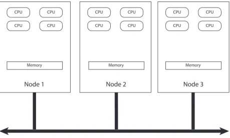
In a distributed memory system, each processor can only work on local data, and explicit communications have to happen whenever they need to access remote data. This is a common architecture on modern computing clusters. A typical structure of a distributed memory system consists of multiple computing nodes (see Figure 1.1), where each node has several processors/cores and a memory that is shared by the processing units on the same node, i.e., each node can be viewed as a shared memory system. The communication between different nodes is achieved through a network such as ethernet or infiniband and viamessage passing paradigms. In contrast to the shared memory system, it is important for each process on a distributed memory sys-tem to know where the data are. The fundamentals of message passing paradigms are send() and receive() functions as well as the identity of different processes. Message Passing Interface (MPI) (see, e.g., [33, 59]) is a standardized and portable message-passing system for writing programs for distributed memory systems.
One major concern in designing message passing algorithms is the performance overhead given by communication between processes. This is especially important
when the number of available processes is huge, or if the amount of computing work allocated to each process is relatively small. In all of our problems, we always neglect the time for a message to be passed between processes. This assumption is valid as long as the computation time on each process dominates, which is the case for the problems considered in this thesis where the tasks on each processor involve solving partial differential equations. However, it should be guaranteed that the message can be sent whenever it is needed. We design and implement our new algorithm following this idea, see Section 3.2 for a detailed discussion.
CPU CPU CPU CPU CPU CPU CPU CPU CPU CPU CPU CPU
Memory Memory Memory
Node 1 Node 2 Node 3
Network
2. SOME EXISTING SAMPLING METHODS
To compute the conditional mean estimator and the conditional covariance esti-mators, it is always necessary to calculate integrals
Eπ(h(x)) = Z
h(x)dπ(x) (2.1)
over the parameter space. In cases where the forward model is complex and the parameter space is of high dimension, computing such integrals analytically becomes infeasible. Traditional quadrature rules also cannot apply because the number of quadrature points grows with dimension. Monte Carlo methods address this issue. The idea of Monte Carlo is to evaluate the target distribution by repeatedly gener-ating random samples from this distribution. Aggregated results are then computed using the ensemble of samples as a discrete approximation of the underlying distri-bution.
The conventional Monte Carlo method draws identically independent (i.i.d.) sam-ples directly from a probability distribution, the central limit theorem guarantees the convergence of the sample expectation value to the real mean value of the sampled distribution at a rate ofO(n−1/2), wherenis the number of samples drawn. However, it is usually infeasible for inverse problems because, in most cases, it is impossible to derive an analytical form for the posterior distribution with which one can draw in-dependent samples. Therefore, advanced random sampling techniques are developed to circumvent the need of sampling directly from the posterior distribution.
In the following sections, we will briefly describe two classes of such algorithms. The importance sampling uses auxiliary distributions that are easier to sample from
to produce independent candidates and then computes a weight for each of these samples. The generated samples, together with their computed weights, is considered a quadrature for any integration under this probability distribution. The Markov chain Monte Carlo (MCMC) uses correlated samples to traverse the sample space and adopts a rejection scheme so that samples of higher probability can be repeated in the ensemble. While the importance sampling method is apparently a parallel algorithm by its nature, it usually performs poorly in practice, especially for complex cases, due to its inability to adjust itself towards regions of interest. On the other hand, MCMC type algorithms are shown in applications to provide the capability of finding the high probability region gradually, but it has to run sequentially to satisfy its Markov chain property.
We will describe both algorithms, discuss the causes for their advantages and disadvantages and some practical ways to measure algorithm efficiency. It is these observations that lead to the idea of our new algorithm in the next chapter, which can be viewed as a hybrid of importance sampling and MCMC, ensuring sampling stability while allowing parallel sampling. In addition, we list some existing parallel MCMC algorithms in Section 2.3.
2.1 Importance sampling methods
The central idea behind importance sampling for a target distribution π(x) is to use an auxiliary probability distribution g(x) that resembles the target while being easy to sample from. Once such a g(x) is constructed, we can rely on the simple change of measure formula for approximation: for anyL1 functionh(x), we will have
Eπ(h(x)) = Z h(x)π(x)dx= Z h(x)π(x) g(x)g(x)dx.
and compute the importance weight
ω(xi) =
π(xi)
g(xi)
. (2.2)
Then, we can build a quadrature with the pairs {xi, ω(xi)}: to estimate the integral of any function h(x) underπ(x), we can use
Eπ(h(x))≈ Pn i=1ω(xi)h(xi) Pn i=1ω(xi) ,
where the appearance of the sum in the denominator is justified by the fact that
ω(xi)’s are usually computed up to a normalization constant, and the effect of this missing constant can be cancelled by also dividing by the sum of ω’s.
It is difficult to accurately measure the efficiency of the importance sampling algorithms. A “rule of thumb” is to use the effective sample size (ESS) to measure the discrepancy between the trial distribution and the target distribution. Suppose a total of n samples is generated using importance sampling, the ESS is defined as
ESS(n) = n
1 + varg[ω(x)],
where varg is the variance of the importance weights. In practice, the variance is estimated through the coefficient of variation defined by
varg[ω(x)]≈ Pn
i=1(ωi−ω)2 (n−1)ω2 , where ω is the sample mean of the weights.
The ESS can be interpreted as the number of samples from i.i.d. draws that can achieve the same accuracy as n importance samples. If the shape of the trial and
target distributions are very different, the variance of the weights can be huge, and thus the ESS can be small, which in turn indicates a poor efficiency in the constructed sampler.
This also reveals the fact that the key to a successful importance sampling lies in the construction of the trial distribution. It has to meet two requirements, namely, it has to be close to the target distribution and we should be able to generate in-dependent samples distributed according to g(x) directly. Both requirements pose challenges to finding satisfying trial distributions for the posterior distributions in Bayesian inverse problems where nonlinearity and high dimensionality are the main features. Therefore, though appearing as a simple and powerful sampling method, importance sampling is rarely applied in Bayesian inverse problems directly. How-ever, its idea of computing the importance weights is borrowed by advanced algo-rithms such as the sequential Monte Carlo [22, 23]. Our new algorithm in the next chapter is also partially inspired by this idea.
2.2 Markov chain Monte Carlo methods
Markov chain theory emerges in the Monte Carlo literature in 1953 by Metropolis [51] to stabilize the parameter space exploration using a random walk dependent on the current state. In 1970, Hastings [36] extended the range of proposal functions from random walk to more general functions. See [55] for a historical summary. Though evidently powerful, Markov Chain Monte Carlo (MCMC) methods did not prevail until the 1990s, mainly due to the lack of efficient computing technology. The visionary work [27] opened doors for MCMC to solving a wide range of problems from biostatistics, physics, geosciences and finance.
2.2.1 Markov chain and its basic properties
To state the fundamental properties of MCMC algorithms, let us first briefly introduce several definitions about Markov chains. A Markov chain is a discrete stochastic process {Xj}that satisfies the following property:
πXj+1(B|xj, . . . , x0) =πXj+1(B|xj),
whereXjis thej-th random variable in the (discrete) process,xj is a realization of the random variable Xj, B is any measurable set andπX is the probability distribution defined by the random variableX. Simply speaking, any state of the random variable
Xj+1 in the process depends on the history of the process only through that of its direct predecessorXj. A transition kernelP :Rn× B →(0,1) defines the probability to move a point xto a Borel setB, andP(x, B) defines atime homogeneous Markov chain {Xj}with the Markov property defined by
πXj+1(Bj+1|xj) =P(xj, Bj+1).
It is called time homogeneous because the transition kernel stays the same for any time index j. In fact, the transition kernel defines the entire process recursively for each of the random variables Xj, j = 1,2, . . . in the process, that is:
πXj+1(B) =πXjP(B) := Z
Rn
πXj(x)P(x, B)dx.
So in contexts we may freely use P to represent the Markov chain it defines. For a given Markov chain with a transition kernel P, a probability distribution π(x) that
satisfies
π(B) = πP(B) := Z
Rn
P(x, B)π(x)dx
is said to be an invariant distribution of P. Later we will demonstrate that a Markov chain with minimal properties will converge to its invariant distribution. This property is the backbone of all MCMC algorithms.
Now we introduce several concepts that characterize Markov transition kernels. A Markov transition kernel P is irreducible with respect to a distribution π if for all x ∈ Rn and B ∈ B with a positive measure under π, there is a k > 0 such that
P(k)(x, B)>0 where we define:
P(k)(x, B) = Z
Rn
P(xk−1, B)P(k−1)(x, xk−1)dxk−1.
Consequently, for any starting point x, and any setB in the support ofπ, we should be able to use P to movex to B in finitely many steps.
For an irreducible kernel P, we say P is periodic if there is a set of disjoint nonempty sets {E1, . . . , Em} ⊂ Rn, m ≥ 2, such that for all j = 1, . . . , m and any
x∈Ej, we haveP(x, E(j+1)mod(m)) = 1. That is to say, a periodic kernel will generate a Markov chain that stays in a loop constantly. We call a kernel that is not periodic an aperiodic transition kernel.
When a Markov chain with transition kernel P satisfies the irreducibility and aperiodicity requirements, which is often true in the designed MCMC algorithms, it has an ergodicity property that is essential to the usability of MCMC:
Proposition 2.2.1. Let π be a probability measure and {Xj} a time homogeneous
measure. Then for π−almost all x∈Rn,
lim N→∞P
(N)(x, B) =π(B) for all B ∈ B,
and for all f ∈L1(π(dx)),
lim N→∞ 1 N N X j=1 f(Xj) = Z Rn f(x)π(dx).
This theorem suggests that to study a probability distribution π(x), we may simulate a realization, denoted as {x1, x2, . . . , xn, . . .}, of a Markov chain P with
π(x) being its invariant distribution. Then, the probability of any Borel set B ∈ B
can be approximated by the relative number of samples in that set regardless of the starting point of this chain. Moreover, the expectation value of any function
f(x) over the distribution π can be approximated by the ergodic average of such a realization, according to the theorem above.
2.2.2 Metropolis-Hastings algorithm
The Metropolis-Hastings algorithm is an MCMC algorithm that forms the basis to many advanced methods. At iteration j, a trial sample x∗ is produced using a proposal function q(xj−1, x∗) where xj−1 is the previous state. The probability distribution π(·) is evaluated at x∗. According to an update formula, the Markov chain chooses to either go to the trial sample (i.e. accept the trial) or merely replicate the previous state (i.e. reject the trial).
Algorithm 1 Metropolis-Hastings Algorithm
Choose a starting point x0. For iteration j = 1,2, . . .
• Propose x∗ using q(xj−1,·),
• compute π(x∗) and compute α(xj−1, x∗) whereα is defined as:
α(x, y) = min 1,π(y)q(y, x) π(x)q(x, y) , • draw u∼U(0,1), If α(xj−1, x∗)≥u letxj =x∗, Else letxj =xj−1.
A commonly used proposal function is the random walk distribution which is a multivariate normal distributionN(xj−1,Σ). In this cases, the proposal is symmetric, i.e., q(x, y) = q(y, x), and the update ratio can be further reduced to α(x, y) = min{1, π(y)/π(x)}. For high dimensional problems, the choice for a fixed covariance matrix Σ is an art. [57] studies this and proposes that the optimal choice of Σ should give an acceptance ratio that is close to 0.234.
The Metropolis-Hastings algorithm has been applied in many inverse problems that require Monte Carlo type samplings. It provides reliable performance thanks to the prudent proposal and update steps that link the adjacent samples. However, the algorithm is computationally very expensive. The number of samples needed
high dimension. In the following, we emphasize two features that result in a large sample number in MH type simulations.
Autocorrelation: Due to the locality of the proposal functionq(x, y), consecutive samples are likely to correlate strongly with each other and hence the ensemble would only have a representating ability equal to that of a much smaller number of independent samples. One of the measures for this intra-chain correlation is the auto-correlation function γj(h) for some function h(x) of interest. It is defined by
γj(h) = 1 (N −j)σ2 N X i=1 h(xi)−h(x) h(xi+j)−h(x) , (2.3)
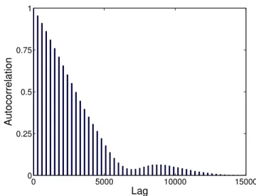
where j is called the lag of the process, σ2 is the sample variance and h(x) is the mean of h(x) over all samples. One practical strategy is to select every k-th sample from the chain where the auto-correlation function γj is small for j ≥ k . This “thinning” procedure can effectively reduce sample correlations and the statistics computed from this subset of samples can be more accurate. We illustrate such an auto-correlation function of a single parameter in Figure 2.1. It comes from chapter 4 where a 64 dimensional parameter is sampled with MCMC method.
Burn-in: At the beginning of the sampling process which starts from an area away from the high probability region, or when the Markov process has not come to the stationary distribution, it will spend several samples to guide itself towards the target region. In practice, this initial segment is called burn-in period and samples in this period are discarded to guarantee a more accurate estimation from the finite number of samples. See Figure 2.2 for an illustration of the burn-in period during sampling.
What adds to the problem of needing many samples in MCMC is that in inverse problems the evaluation of each sample is expensive because the forward model
in-0 5000 10000 15000 0 0.25 0.5 0.75 1 Lag Autocorrelation
Figure 2.1: Auto-correlation function for one of the 64 estimated parameters. Judg-ing from this plot, we may need to use a“thinning”of 10,000 samples, that is, picking every 10,000th sample in the sequence to compute any estimate.
0 1 2 3 x 10⁴ 0 3 6 9 Samples ¯ x
Figure 2.2: An illustration of the burn-in period during sampling. In this example, the true value of the parameter is 1. It is advised to discard the first 104 samples to have a more accurate mean estimator. But this means we have to abandon 1/3 of the total computing effort.
volves solving the underlying partial differential equations. For example, in the opti-mal tomography example in chapter 5, a single evaluation costs about 41.5 seconds, and it takes us about 29 days to collect 60, 000 samples with MCMC. Although parallel computing has become an important means of acceleration and many al-gorithms have been successfully parallelized, the study of MCMC parallelization is relatively scarce. This is mainly due to the sequentiality of the algorithm where new samples can not be generated until after the accept-reject decision has been made for the current sample. This motivates our research to design new frameworks that enable running MCMC in parallel.
To summarize, in order to make MCMC more tractable for large scale inverse problems, we need to either increase the statistical efficiency of the algorithm or modify the algorithm so that it can be run in parallel. In the following section, we will describe an adaptive MCMC algorithm which could help improve the statistical efficiency of the algorithm. It is worth noting that this technique can be readily incorporated in our new framework introduced in Chapter 3.
2.2.3 Adaptive proposal for Metropolis-Hastings
To ameliorate the slow mixing of random walk Metropolis-Hastings, [35] proposes an adaptive method. In contrast to the plain random walk that always proposes new samples according to the same normal distribution, this method will adapt the proposing distribution using the statistics of past samples. Through this adaptation, we can hope to approximate the shape of the target distribution function around the current sample, thus increasing the chances to land on a state superior than the current one. More specifically, suppose the Markov chain has already generated samples {x1, x2, . . . , xn}, the proposal function for the next sample will be a normal
distribution with mean vector µn = 1 n n X i=1 xi
and covariance matrix Σnwhich is the sample covariance of alln past samples. Since Σn is defined as Σn = 1 n−1 n X i=1 xixTi − n n−1µnµ T n,
we can update this matrix in a fast recursive way through
Σn= n−2 n−1Σn−1+µn−1µ T n−1− 1 n−1(nµnµ T n −xnxTn).
The proposal function is then chosen to be a normal distribution with the covariance matrix:
Σupdate =sd(Σn+N(0,1)Id),
where d is the dimension of the parameter space, sd is empirically chosen to be (2.38)2/d. The N(0,1)Id term is a “safety measure” that prevents the update covariance matrix from being singular.
We use the following procedure to compute new proposals which should then give the multivariate normal distribution N(µn,Σupdate): at each iteration, we first perform a Cholesky decomposition for the update covariance matrix Σupdateto obtain a lower triangular matrix Lwhere L satisfies
LLT = Σupdate,
form X∗ =Xn−1+LZ. In fact, it is straightforward to check that
E(X∗) = E(Xn−1+LZ) =Xn−1,
and that
Σ(X∗) = E(LZZTLT) =LLT = Σupdate.
The adaptive proposal has many applications and is adopted to increase sam-pling efficiencies in Bayesian inverse problems, for example, in [20]. Together with a delayed-rejection scheme, they constitute the delayed-rejection adaptive Metropolis (DRAM) algorithm [34]. It has been used as a reference algorithm to compare newly developed advanced, single chain MCMC algorithms, for example, in [49]. Theo-retically, since the adaptive proposal incorporates information regarding the entire history, rather than the most recent sample, it imposes some difficulty in analysis. It is only until recent years that convergence rates of such adaptive algorithms are estimated. See [4, 56] for a discussion on the theory of the adaptive algorithm.
2.2.4 Diagnostic tests for MCMC algorithms
The convergence of a Monte Carlo method using independent and identically distributed random variables is provided by the classical central limit theorem, saying that the error is bounded byO(1/√n), wherenis the number of independent samples. On the other hand, it is much more difficult to estimate whether a Markov Chain has converged. Correlation between successive samples in a Markov chain introduces uncertainty, giving difficulty to any attempt of drawing a comprehensive conclusion. To date, there is yet any theoretical support to give a good estimate over this issue in general. However, numerous diagnostic tools exist to test the convergence property of Markov chains in practice. What these examiners do is, rather than assuring that
a chain has already converged, telling that a chain has not reached stationarity. As long as these examiners tell “no” we have to let the chain run longer. In addition, the diagnostic can also verify the speed of mixing of a chain. If a chain is developed in the manner that no matter where we start the chain, it could direct itself to stationarity quickly, the examiner will be able to indicate such a chain as a “good” one. In the paragraphs below, we will briefly review a few diagnostic methods and then detail the convergence standard we prefer in our numerical experiments.
A good overview of such diagnostic tools is [19]. Among the different testing methods, a popular one is the Potential Scale Reduction Factor (PSRF) derived in [28]. Multiple chains are started from different positions that are far away from each other (being “overdispersed”). At convergence, the histograms of each variable from different chains should overlap considerably.
The formal definition of PSRF for a one dimensional variable is as follows. m
chains are started from different points, with each generating 2n samples. The last
n samples are picked, and the within-chain variance W and between chain variance
B/n are computed by W = 1 m(n−1) m X i=1 2n X j=n+1 (xij −x¯i)2 and B/n = 1 m−1 m X i=1 (¯xi−x¯)2,
where ¯xi is the average of lastnsamples from chain iand ¯xis the average of all ¯xi’s. Taking both the within chain and between chain variances into account we obtain
an estimate of the posterior variance which is defined as ˆ V = n−1 n W + (1 + 1 m) B n,
and the PSRF factor ˆR is defined through dividing this variance by W:
ˆ
R =
ˆ
V W.
When the chain has converged, the factor will be close to one, which makes it a nice criterion for monitoring convergence. However, this factor is unidimensional, namely, it can merely monitor the behavior of a single variable at once. In order to obtain an integrated view of the convergence of all variables, [15] extended the criterion to multivariate situations. The Multivariate Potential Scale Reduction Fac-tor (MPSRF) is defined similarly to its univariate sibling, with scalar values being replaced by multidimensional vectors, and variances replaced by covariance matrices
W = 1 m(n−1) m X i=1 n X j=1 (xij −x¯i)(xij −x¯i)T and B/n= 1 m−1 m X i=1 (¯xi−x¯)(¯xi−x¯)T.
The definition of ˆV as a combination ofB andW is as before, whereas the definition of ˆR becomes a bit different because now we have to define a proper division for
covariance matrices. [15] defines it as the generalized Rayleigh quotient ˆ R = max a ( ˆV a, a) (W a, a) = n−1 n + m+ 1 m maxa (B/na, a) (W a, a) = n−1 n + m+ 1 m λmax,
whereλmax is the largest eigenvalue ofW−1B/n for positive definite matricesW and
B/n.
One feature of the PSRF and MPSRF diagnostics is that multiple chains have to be run from different starting points and it can be time consuming if an online diag-nostics is required. Especially, in the context of parallel computing, communication between these multiple chains is demanded to summarize the statistics, which could put an overhead to the algorithms. This is avoided in the alternative estimator—the mean squared error (MSE) estimator [17] that is defined as
M SE(x) = Ex(x−x∗)2
= Varxx+ (Exx−x∗)2,
whereEx means taking the sample average andx∗is the true parameter. The second equation indicates that the MSE includes both the variance of estimate and the bias of an estimator to its true values.
In problems with real data, the true parameter x∗ is in general unknown, and hence it is impossible to directly apply the MSE formula for estimation. In Bayesian inverse problems, even if we generate the synthetic data using a reference parameter, since we also incorporate a prior distribution, the mean value of the posterior distri-bution may not be the same as the true parameter. Therefore, if MSE were used as
a convergence criterion and the error of a sampling scheme did not converge to zero, it would be difficult to tell whether it stems from a poor converging sampler or from the modeling bias.
To circumvent this dilemma so that we can merely compare the convergence performance of different samplers, we make some efforts to exclude the modeling discrepancy. To achieve this, we may run an MCMC chain for a sufficiently long time which we believe to have converged. We then compute the sample mean x∗
and the sample covariance Σ out of this long chain. Then, we are able to compute the error as a weighted mean square error which we call the Empirical Mean Square Error: EM SEn(x) = Ex(x−x∗)2Σ−1 = 1 n Pn i=1(xi−x ∗)TΣ−1(x i−x∗). (2.4)
The reference Markov chain is long enough so that we can believe that the x∗ is as close to the expected value of the posterior distribution as the best of any other sampler we want to evaluate. Also, the Σ quantifies how much uncertainty there is in the model itself. For example, if the physical experiment is designed such that we are only able to observe data from the surface of an object, it is likely that our model may behave more poorly for inferring parameters deep inside the object which then could indicate a bigger variance for internal parameters in the covariance matrix Σ. It is then legitimate to assume that such uncertainty will live in any sampling method as long as they are sampling the same model. Therefore, by weighing the errors with the inverse of the covariance matrix, we can hope to eliminate some uncertainties from modeling and concentrate on the error brought about by the samplers themselves.
Another useful diagnostic test is to compute the integrated autocorrelation time (IACT) [48] which is defined as (again, for some function h(x) of the random
vari-ables) τ(h) = 1 + 2 ∞ X j=1 γj(h), (2.5)
where γj is the autocorrelation function defined in (2.3). This number is related to the effective sample size (ESS) defined for correlated samples, which, for a total of
n samples, has the expression
ESS = n
2τ(h). (2.6)
The ESS is a description of the number of independent samples which have similar estimated statistics as that of the n (potentially correlated) samples. Therefore, the smaller the IACT is, the larger the ESS is, and hence we may say that the sampler is possessing a better statistical efficiency. In later chapters, we will show how to use EMSE and IACT to measure the performance of different samplers. We will also show that the concept of effective sample size can help us properly quantify the speedup of an MCMC algorithm in parallel computing.
2.3 Existing parallel MCMC algorithms
The most straightforward strategy to use MCMC in parallel is to generate mul-tiple chains starting from points that are far away from each other [28]. Samples are then collected from all the chains to achieve a bigger ensemble of samples than a single chain could achieve within the same amount of wall time. However, there are several practical problems with this setting. First of all, there is no clear criterion to tell whether the starting points have spread far away from each other. It is quite possible that different starting points soon lead the sampler towards a common re-gion of interest and each of the multiple chains only manage to sample this rere-gion due to limited number of samples. Samples from different chains are then correlated across chains and the convergence could be slowed. In contrast, a single long chain
might have a better chance of ergodicity. In addition, every chain has to discard the burn-in period whose length is non-uniform (because of the different starting points) and hard to estimate. One strategy is to discard a fixed, but large enough, number of samples for each chain, which means that the number of wasted samples grows proportionally to the number of chains available. All these could reduce the gains from the multiple chain implementation. See [29] for a detailed discussion.
In the following, we will discuss two other parallel MCMC algorithms. They represent two categories of ideas behind the parallelization of MCMC: the single chain parallelization and the multiple chain parallelization. We discuss both the improvements they make and the obvious limitations they possess.
2.3.1 Prefetching MCMC algorithm
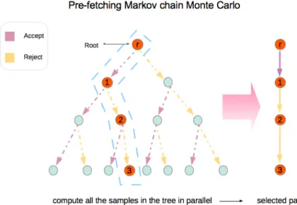
A single-chain parallelization strategy called the prefetching MCMC was pro-posed in [13]. When multiple processors are accessible, it is possible to propose, on the main processor, the candidates for several steps ahead using a computationally inexpensive random walk type distribution. These candidates are then distributed to several processors and can be evaluated simultaneously. Once their probability density function values are computed and sent back to the main processor, the main processor can then perform a series of accept-reject decisions for acquiring multiple samples in the Markov chain. We further illustrate the details of the idea by showing an example of prefetching MCMC that uses a total of 7 processes. In this illustration, we use a binary tree structure to demonstrate the conceived stages: for each node in the tree, the left child stands for the new candidate and the chain will go to left if an “accept” decision is finally made upon it; the right child, on the other hand, stands for the result of the “reject” decision and hence it is an identical sample as its parent.
Example 2.3.1. At the current sample xj, we use seven processors to extrapolate three levels at the same time. Firstly, on the main processor, a tree of new samples are spawned using a random walk type proposal function. Each left child of a node is a new candidate while the right child is identical to its parent, as is demonstrated in Figure 2.3. Then, all that needs to be computed is the probability density function value (expensive step) at the seven nodes on level three except for the rightmost one on different processors in parallel. Once these values are gathered, on the main processor, starting from xj, the root, we perform a sequence of Metropolis Hastings updates and get three new samples xj+1, xj+2 and xj+3. This algorithm is robust in the sense that we will always obtain three new samples. We still end up with one single chain that is identical to the original single-processor algorithm. The mixing rate and the burn-in both remain intact.
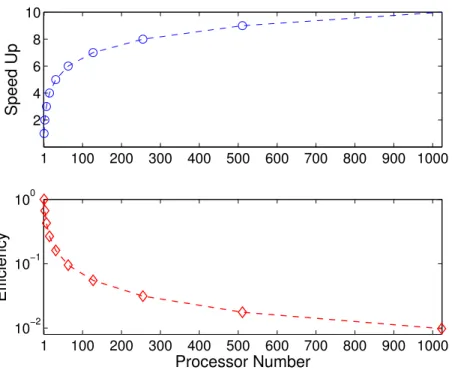
upper limit of its speed up is log2(P + 1), where P is the number of the processors available. In Figure 2.4 we show the theoretical speed up and the efficiency, the ratio of the speed up over the number of processors available. As can be seen from the plot, the algorithm scales poorly with the number of processors. Besides, the implementation of this algorithm also relies on a fixed, computationally inexpensive proposal distribution such as the random walk, as the candidates are all generated on the main processor and only the evaluation of π(x) is parallelized. For advanced MCMC algorithms such as the multiple try Metropolis algorithm [47] where the anchor point for new proposal is undecided until after evaluation is taken place, or the Stochastic Newton’s method [49] where each new sample is proposed by solving an optimization problem, the prefetching algorithm cannot be directly applied.
2.3.2 Parallel tempering method
As is discussed above, plainly running multiple chains of MCMC may not be an ideal solution of algorithm parallelization. In this section, we discuss another multiple chain strategy, theparallel tempering (PT) algorithm [24], that allows between chain interactions. These interactions empower Markov chains to jump between states rather than being trapped in local optima, and they increase statistical efficiencies in general.
The parallel tempering algorithm deals with a product spaceX1× X2×. . .× XI, with each Xi being an identical copy of the original parameter space X. A joint probability distribution
π(x1, . . . , xI) = Y
i∈I
πi(xi)
is assigned to the product space. In implementation, the I chains are run in parallel and the algorithm is defined as:
1 100 200 300 400 500 600 700 800 900 1000 2 4 6 8 10 Speed Up 1 100 200 300 400 500 600 700 800 900 1000 10−2 10−1 100 Processor Number Efficiency
Figure 2.4: Theoretical speedups and efficiencies of the prefetching algorithm for different number of processors. Since in the inverse problems the computing time dominates the communication time, these theoretical estimates should be close to the data from numerical experiments.
Algorithm 2 Parallel Tempering Algorithm
• Let the current state be {x(t)1 , . . . , x(t)I }; draw u∼Uniform[0,1],
• Ifu≤α0, we update eachx(t)i tox(t+1)i by using a Metropolis-Hastings strategy,
• Ifu > α0, we perform a swapping step, i.e., we randomly choose a neighboring pair, say i and i+ 1, and swap x(t)i , x(t)i+1 with probability
min ( 1,πi(x (t) i+1)πi+1(x (t) i ) πi(x (t) i )πi+1(x (t) i+1) ) .
In parallel tempering, theπi’s are chosen as a sequence of “tempered” distribu-tions, namely,
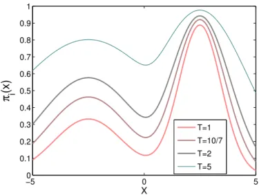
πi(x)∝exp{logπ(x)/Ti}= (π(x))1/Ti, (2.7) where 1 = T1 < T2 < . . . < TI and π1 is set to be the original distribution. The above form is similar to the Boltzmann distribution in physics where −logπ1(x) serves as the energy and T as the temperature, the setting is hence named. See Figure 2.5 for an example of a sequence of tempered mixed Gaussian distributions. Intuitively, as the temperature increases, the distribution will be more flattened, i.e., the barriers between different regions become smaller, thus allowing the sampler to traverse different areas of the parameter space more easily. When the samples of the original distribution are trapped around a local peak, those sampling the higher temperature distributions may have reached another region of interest. The swap steps in the algorithm permit exchanging information between the states at different energy levels and help the chain on the original distribution to mix faster.
−50 0 5 0.1 0.2 0.3 0.4 0.5 0.6 0.7 0.8 0.9 1 X π i (x) T=1 T=10/7 T=2 T=5
Figure 2.5: A sequence of (unnormalized) tempered density functions for a mixed Gaussian distributions.
A practical issue in implementation lies in the tuning of the temperature ladder. An empirical conclusion is that one should start with choosing the highest tempera-ture. It should be chosen to allow exploring the whole space rather easily, i.e., with a high acceptance ratio (α > 0.9). Then the lower temperatures are chosen such that their histograms overlap to some degree with its closest neighbor, see [48] and [45] for detailed suggestions. One of the criteria for a good temperature ladder is that the swapping step should be accepted with a ratio of approximately 50%. A too small swap rate means an inefficient exchange of information, while a too big swap rate will interupt the local search very frequently that can result in a much blurred image of the target distribution.
While the parallel tempering algorithm is able to accelerate MCMC sampling by increasing the mixing rate, it has a limitation in using multiple processors, namely, we can only use the number of processors that are equal to the number of chains. To
total. It has been advised that fewer than ten chains shall be used. That is to say, only ten processors can be fully exploited at most.
3. THE MARKOV CHAIN PRECONDITIONED MONTE CARLO METHOD
The existing parallel MCMC algorithms explored single chain and multiple chain parallel schemes, but the efficiency in terms of parallel computing is very limited. This is due to the sequential nature of MCMC that the proposal of each sample relies on the information of the previous state. It is then attractive to study theindependent Metropolis-Hastings algorithm which proposes new samples using a distributionq(x) that does not rely on samples for the target distribution π(x). The main problem with this idea is that whenever the proposal distribution is not close enough to the target distribution, the proposed samples are most likely to fall in regions of low target probability and the acceptance ratio of such algorithms can be extremely small. This problem becomes more severe when the dimension of the parameter space is high. In such cases, the high probability regions only fill a very small portion of the space.
3.1 The MCPMC algorithm
Inspired by the “interacting Markov chain Monte Carlo” in [14], we derive a new algorithm that is able to remedy this problem. Instead of choosing a proposal function which has no knowledge of the posterior distribution, we construct it by using approximation models of the posterior distribution. For example, we may construct the posterior distribution on a less accurate but much faster solver for the forward problem. When the forward problem is about solving a partial differential equation, we may discretize the equation by using a coarser grid. The posterior built this way will be easier to evaluate, while through a careful treatment we can keep the distribution built on the coarser grid close enough to the accurate model.
trievable in an analytic form, therefore we may sample the approximation using some MCMC method. Sampling this distribution is then much faster than sampling the real distribution. While the approximation model is sampling, we randomly select samples from the expanding pool, taking the growing ensemble as a discrete proposal distribution. As more samples are generated from the proxy model, this ensemble should resemble the approximate distributionπapprox(x) and the random selection can be considered as if they come straight from an independent draw from πapprox(x).
Then, proposed candidates are evaluated independently on different processes to compute an importance weight following equation (2.2)
w(x) = π(x)
πapprox(x)
.
Comparing the weight of a new proposal and of the current sample, we update the chain for real posterior distribution following the Metropolis-Hastings algorithm. Roughly speaking, this step filters out the samples that have a relatively small value on π(x) and replicates the samples whose weight evaluation are large.
Even though the approximate model can be crafted to be close to the accurate model, they are not identical. Thus, samples from the approximate model may not cover the entire high probability regions of the accurate model. Taking this fact into account, we add a step to the new algorithm which uses a short Markov chain with invariant distribution π(x) to perturb the samples towards a higher probability area. The last sample obtained from this short chain then replaces the acquired sample. The computation of each short chain is expensive because it may incur several forward model evaluations. But since every such chain can be run entirely in parallel the additional cost can be effectively controlled with a sufficient number of processors.
It is also noteworthy that the preconditioning can be readily extended to multiple levels of approximations rather than having only one approximation πapprox(·) and one accurate model π(·). For example, to guarantee a smoother transition from the approximate to the accurate, we may insert several intermediate chains whose density functions are weighted geometric means of the approximate and accurate models. That is, we can choose intermediate distributions πλ(x) according to
πλ(x) =πapprox1−λ (x)π
λ(x), λ∈(0,1).
By carefully choosing a sequence of such temperatures, we will be able to make neighboring distributions close to each other. Refer to [43] for an example of using this setup in a sequential Monte Carlo (SMC) sampling.
As the new algorithm is derived from the interacting MCMC, they share a the-oretical basis. Meanwhile, the new algorithm differentiates itself from the original in aspects. The interacting MCMC algorithm is built for state space models where multiple chains are built on parameter spaces with increasing dimensions (i.e., a se-quence ofaugmenting spaces). In the state space models, transitions between succes-sive spaces have already been defined as conditional distributions. In our framework, however, there is only one parameter space with a fixed dimension across all the chains. To fit into the same algorithmic framework, we need to build approximation models and sample the approximate distribution as an auxiliary. Since there is no natural transition from the approximate to the accurate, we add the Markov kernel based perturbation step to connect both models. A similar algorithmic modification appeared in [22, 23]. Therein, the authors modified an SMC method which is origi-nally designed for general state space models of increasing parameter dimensions to
uses Markov chains instead of relying on independently generated samples, hence we can expect better asymptotic stability.
Note that in this algorithm, we use a coarse model to guide the simulation on a fine model, and the Markov chain is mainly used for sampling the approximation distribution, we realize that the coarse model Markov chain can be viewed as a stochastic approximation of the approximation distribution which then serves as a preconditioner for sampling the true distribution. Hence, we name it the Markov chain preconditioned Monte Carlo method. In the following, we give the formal description of the algorithm in a general multiple chain version. For conciseness, we show the algorithm in a synchronous way, that is, we assume that for every iteration both the preconditioning chain and the target chain produce exactly one sample. In real implementations, nevertheless, the speed of the two chains depend on factors such as the number of processors we use and the number of perturbations after each update.
Algorithm 3 Markov chain preconditioned Monte Carlo
Suppose there are n chains with πn(x) = π(x) and πi(x), i = 1,· · · , n −1 is a sequence of approximations. At iteration k, do:
• For chain i= 1, updateXk
1 using a traditional MCMC with invariant distribu-tion π1(x),
• For chain i= 2,· · · , n, do the following steps
– Select: randomly propose a sample Xim−1, m ∈ [1, k] from the previous chain as Xi∗,
– Update: compute the incremental weightwi(Xi∗) :=πi(Xi∗)/πi−1(Xi∗) and make update decision with probability
αi(Xi∗, X (k−1) i ) = min 1, wi(Xi∗) wi(Xi(k−1)) ! = min 1,πi(X ∗ i)πi−1(X (k−1) i ) πi−1(Xi∗)πi(X (k−1) i ) ! ,
– Perturb: moveXi∗ by a Markov kernel with invariant distributionπi(·) to
Xik.
This algorithm is well suited for parallel computing in that sample proposals for the i-th chain where i ≥ 2 can be done in parallel: it is easy to select multiple candidates from the previous chain, evaluate them on different processors (expensive step), make the sequential update decisions and perturb those accepted samples again in parallel. That is to say, all the expensive steps, the before-update evaluation and