University of Zurich
Zurich Open Repository and Archive
Winterthurerstr. 190 CH-8057 Zurich http://www.zora.uzh.ch
Year: 2010
A score regression approach to assess calibration of continuous
probabilistic predictions
Held, L; Rufibach, K; Balabdaoui, F
Postprint available at: http://www.zora.uzh.ch
Posted at the Zurich Open Repository and Archive, University of Zurich. http://www.zora.uzh.ch
Originally published at:
Biometrics 2010, 66(4):1295-1305.
Held, L; Rufibach, K; Balabdaoui, F (2010). A score regression approach to assess calibration of continuous probabilistic predictions. Biometrics, 66(4):1295-1305.
Postprint available at: http://www.zora.uzh.ch
Posted at the Zurich Open Repository and Archive, University of Zurich. http://www.zora.uzh.ch
Originally published at:
A score regression approach to assess
calibration of continuous probabilistic predictions
L. Held
Biostatistics Unit, Institute for Social and Preventive Medicine, University of Zurich, Hirschengraben 84, 8001 Zurich, Switzerland
*email:[email protected]
and
K. Rufibach
Biostatistics Unit, Institute for Social and Preventive Medicine, University of Zurich, Hirschengraben 84, 8001 Zurich, Switzerland
*email:[email protected]
and
F. Balabdaoui
Universit´e Paris Dauphine, Centre de Recherche en Math´ematiques de la D´ecision, Place du Mar´echal de Lattre de Tassigny, 75775 Paris 16, France
*email:[email protected]
Summary: Calibration, the statistical consistency of forecast distributions and the observations, is a central requirement for probabilistic predictions. Calibration of continuous forecasts is typically assessed using the probability integral transform histogram. In this paper we propose significance tests based on scoring rules to assess calibration of continuous predictive distributions. For an ideal normal forecast we derive the first two moments of two commonly used scoring rules: the logarithmic and the continuous ranked probability score. This naturally leads to the construction of two unconditional tests for normal predictions. More generally, we propose a novel score regression approach, where the individual scores are regressed on suitable functions of the predictive variance. This conditional approach is applicable even for certain non-normal predictions based on the David-Sebastiani score. Two case studies illustrate that the score regression approach has typically more power in detecting miscalibrated forecasts than the other approaches considered, including a recently proposed technique based on conditional exceedence probability curves.
January 2006
Key words: Calibration; Cross-validation; Continuous predictions; Scoring rules; Regression.
c
1. Introduction
Calibration of probabilistic forecasts is defined as the statistical consistency of forecast distributions and the observations (Gneiting et al., 2007). Good calibration is a central requirement for probabilistic predictions, both from a frequentist (Cox, 1958; Butler, 1986) and a Bayesian (Dawid, 1982) perspective.
Calibration of probabilistic forecasts can be evaluated in different ways. For binary fore-casts, various inferential and graphical techniques have been suggested in the literature (Sanders, 1963; Copas, 1983; Spiegelhalter, 1986; Hosmer and Lemeshow, 1989; Schmid and Griffith, 2005), some of them based on the famous Brier score (Brier, 1950). For evaluation of predictions in survival we refer to Graf et al. (1999); Schumacher et al. (2003); Gerds et al. (2008). These techniques are increasingly used in clinical epidemiology and other fields, see e.g. Harrison et al. (2007); Lix et al. (2008); Steyerberg (2009).
For univariate continuous forecasts, calibration is traditionally assessed in a more ex-ploratory manner, using the probability integral transform (PIT) histogram (Dawid, 1984). Alternatively, strictly proper scoring rules may be used that allow both the sharpness and the calibration of the predictive distribution to be evaluated (Gneiting and Raftery, 2007). A general systematic discussion of different notions of calibration for probabilistic forecasts of continuous variables is given in Gneiting et al. (2007).
Usually, in evaluating continuous forecasts, strictly proper scores are computed but no formal significance test is performed to determine whether the computed value of the scores considered provides evidence of lack of calibration of the predictive distribution. In this paper we present significance tests based on scoring rules to assess calibration of continuous pre-dictive distributions. For normal predictions we consider the logarithmic and the continuous ranked probability score (LS and CRPS, respectively). Note that both these scoring rules are proper (Gneiting and Raftery, 2007), however, propriety is not explicitly used in our
approach. We study properties of these two scores if the observation is a realisation from the predictive distribution. In that case the forecast is called ideal and is strongly calibrated in the terminology of Gneiting et al. (2007). For an ideal normal forecast we derive the first two moments of these two scores to set up two unconditional tests to assess strong calibration.
These tests are direct generalizations of Spiegelhalter’s z-test (Spiegelhalter, 1986; Schmid
and Griffith, 2005) for calibration of binary predictions based on the Brier score to the setting of normal predictions.
The logarithmic score for normal predictions can be seen as a special case of the
Dawid-Sebastani score(DSS) (Dawid and Sebastiani, 1999; Gneiting and Raftery, 2007; Czado et al., 2009; Riebler and Held, 2009), which is based on the first two moments of the predictive distribution. If these two moments match the corresponding moments of the data-generating distribution, the expectation of DSS depends only on the log predictive standard deviation in a known functional form. This fact can be used for a more powerful score regression approach, which is applicable even for certain non-normal predictions. A score regression approach based on the CRPS is also suggested, which is useful not only for normal predictions, but also for any other location-scale family of distributions.
We introduce some notation. Letf(.) andF(.) denote the density and cumulative
distribu-tion funcdistribu-tion, respectively, of the probabilistic forecast Y. The actual observation is denoted
by yobs. For continuous predictions, the most prominent scoring rules are the logarithmic
score
LS(yobs) = −logf(yobs)
and the continuous ranked probability score
CRPS(yobs) = E|Y1−yobs| −E|Y1−Y2|/2,
compare Gneiting and Raftery (2007). Here Y1 and Y2 are independent random variables
We first consider the important case of a normal prediction Y ∼ N(µ, σ2), in which case the logarithmic score becomes
LS(yobs) =
1
2{log(σ
2) + ˜y2
obs}, (1)
where ˜yobs = (yobs −µ)/σ and the constant log(2π)/2 has been omitted. Under normality,
the continuous ranked probability score turns out to be
CRPS(yobs) = σ[˜yobs{2Φ(˜yobs)−1}+ 2ϕ(˜yobs)−1/
√ π],
compare Gneiting et al. (2006). Here and throughout, ϕ(.) and Φ(.) denote the density and
the cumulative distribution function, respectively, of a standard normal distribution.
If we specify the predictive distribution only through the first two (finite) moments µand
σ2, the Dawid-Sebastani score as proposed in Dawid and Sebastiani (1999) has (up to a
multiplicative constant) the same form as the logarithmic score (1) under normality:
DSS(yobs) =
1
2{log(σ
2) + ˜y2
obs}. (2)
In Section 2 we study properties of DSS(Yobs), LS(Yobs) and CRPS(Yobs) for ideal forecasts.
For DSS, an “ideal” probabilistic forecast is to be understood as one with first two moments matching the true moments of the data-generating process. Of course, equality of the first two moments does not necessarily imply that the forecast distribution equals the data-generating distribution. In Section 3 we construct two unconditional test statistics based on LS and CRPS to assess calibration of normal predictions. In Section 4.2 we propose a more powerful score regression approach based on DSS and CRPS, where the individual scores
are regressed on suitable functions of the predictive variance σ2 and which is also applicable
for certain non-normal predictions. In a simulation study, the performance of the new tests is contrasted with tests for uniformity of the PIT values and a recently proposed technique based on conditional exceedence probability curves that is described in Section 4.1. All tests outperform the Kolmogorov-test for uniformity of the PIT values. The various tests are
further illustrated using a real life application from forensic medicine. In Section 6 we close with some discussion and outline possible extensions to multivariate forecasts.
2. Properties of DSS, LS and CRPS for ideal forecasts
Assume that mean and variance of the data-generating distribution of Yobs equal the mean
and variance of the distribution of the forecast Y. From (2) it immediately follows that
E{DSS(Yobs)} = 1/2 + logσ. (3)
No normality assumption is needed for this result, it holds for any predictive distribution
with finite second moment. Note that both E{DSS(Yobs)} and DSSmin = logσ, the smallest
possible value of DSS, depend on the logarithm of the predictive standard deviation σ. The
variance of the DSS does not depend on σ and is finite, provided the fourth moment ofYobs
is finite. Under normality, it is immediate that
Var{DSS(Yobs)} = Var{LS(Yobs)}= 1/2. (4)
Obtaining expectation and variance of the CRPS of an ideal forecast is difficult in general, but possible for normal forecasts. It is useful to write the CRPS more explicitly as
CRPS(yobs) = E(Z|Yobs =yobs)−E|Y1 −Y2|/2,
where Z = |Y1−Yobs|. We are now interested in the expectation and the variance of the
CRPS, viewed as a function of the random variable Yobs ∼ N(µ, σ2). The law of iterated
expectation states E E(Z|Yobs) = E(Z) = E(|Y1−Yobs|), so
E{CRPS(Yobs)} = E(|Y1−Yobs|)−E|Y1−Y2|/2 = E|Y1−Y2|/2,
since Y1,Y2 andYobs are independent and identically distributed. As shown in the Appendix,
it follows that |Y1−Y2| is half-normally distributed with expectation 2σ/
√ π, so
E{CRPS(Yobs)} = σ/
√
π. (5)
pro-portionality constant 1/√π. Note that this is also the case for the lower bound CRPSmin =
σ·(√2−1)/√π, only the proportionality constant differs.
The proportionality of E{CRPS(Yobs)} to σ =
p
Var(Yobs) in (5) does not only hold for
normal distributions, but generally for all location-scale families that are associated with a
standard density f0 with finite standard deviation σ0, say. To see this, let Xobs, X1 and X2
be independent random variables with density f0. Then E{CRPS(Xobs)}= E|X1−X2|/2 is
c·σ0, say, for somec >0. All membersY of the location-scale family can be written as linear
transformations of a random variable with standard density f0, so let Yobs =a+bXobs, Yi =
a+bXi, i= 1,2 fora∈R and b >0. Of course, σ =
p
Var(Yobs) =b·σ0. Then,
E{CRPS(Yobs)} = E|Y1−Y2|/2
= bE|X1−X2|/2
= bE{CRPS(Xobs)}
= b·c·σ0 = c·σ.
For example, the uniform distribution is such a location-scale family with proportionality
constant c = 1/√3. For the derivation of the test statistic (11) it is important to note that
the dependence of E{CRPS(Yobs)}onσis not only linear for the general location-scale family,
but that E{CRPS(Yobs)} is proportional to σ, i.e. the intercept of the linear relationship is
zero.
In the appendix, we show that under normality
Var{CRPS(Yobs)} = ³1 3 − 4−√12 π ´ ·σ2 = C·σ2
with C = 0.16275. . .. This result is needed for the unconditional calibration test described
in Section 3. Similar arguments as above can be used to show that Var{CRPS(Yobs)} is
3. Two unconditional calibration tests for normal predictions
Suppose that i = 1, . . . , n independent normal predictions have been made with predictive
mean µi and variance σ2i. Based on the actually observed values yobsi, i = 1, . . . , n, the
corresponding LS values LSi and CRPS values CRPSi have been computed. Let LS =
n−1Pn
i=1LSi denote the mean logarithmic score and CRPS = n−1
Pn
i=1CRPSi the mean
CRPS.
The results from the previous section suggest to construct test statistics of the form
zLS = {LS−E0(LS)}/Var0(LS)1/2 and zCRPS = {CRPS−E0(CRPS)}/Var0(CRPS)1/2.
Here E0(LS) = 1/2 + 1 n n X i=1
log(σi) and Var0(LS) = 1/(2n)
are the mean and variance of the mean logarithmic score LS of an ideal normal forecast, compare (3) and (4). Similarly,
E0(CRPS) = 1 √ π 1 n n X i=1 σi and Var0(CRPS) = C n2 n X i=1 σ2i
are the mean and variance of CRPS of an ideal normal forecast. Due to standard arguments,
zLSandzCRPS are approximately standard normal test statistics for ideal forecasts. We reject
the null hypothesis of calibration for large values of |zLS| and |zCRPS|, respectively.
These proposed tests for normal predictions naturally complement Spiegelhalter’sz-statistic
(Spiegelhalter, 1986) for binary predictions based on the Brier score, as implemented for
example in the functionbrierinSTATA(StataCorp., 2003). The above tests are unconditional
in the sense that they average over the individual scores regardless of the underlying predic-tive distributions. For normal predictions they provide an alternapredic-tive to tests for uniformity of
the probability integral transform PIT(yobsi) = Fi(yobsi) = P(Yi 6 yobsi), see Dawid (1984)
and Gneiting et al. (2007). Indeed, for an ideal forecast PIT(Yobs) is standard uniformly
et al., 2009). Standard statistical tests, such as the Kolmogorov-test, can then be used to investigate uniformity of the PIT of a sample of independent predictions.
However, the two unconditional tests have two distinct disadvantages. First, the expec-tation and variance of the considered score must be known. Secondly, they average over the scores regardless of the predictive distribution. In Section 4 we describe two regression approaches which condition on characteristics of the predictive distribution. These techniques provide more powerful tools for the detection of miscalibration and are applicable even for certain non-normal predictions.
4. Regression approaches
The first approach to detect miscalibration of a probabilistic forecast using regression is described in Cox (1958). However, Cox’s approach is only applicable to binary predictions, see also the discussion in Miller et al. (1991, Section 2.4).
In the case of continuous predictions, we now describe two regression approaches which condition on characteristics of the forecast distribution. The first approach, proposed by Mason et al. (2007), conditions on a specific quantile of the predictive distribution, for example the median. Logistic regression is used to investigate if conditional exceedence probabilities depend on the magnitude of the chosen quantile. Motivated by the results of Section 2, in Section 4.2 we propose regressing the individual score contributions on functions of the predictive variance to obtain an alternative method to detect miscalibration.
4.1 Logistic regression of conditional exceedence probabilities
Mason et al. (2007) suggested the usage of conditional exceedence probabilities (CEP) to assess calibration of probabilistic forecasts. The approach can be described as follows. Let
then Yobs is distributed according toF as well, so the conditional exceedence probability
P{Yobs > q(p)} (6)
equals 1−p for any given p ∈ (0,1). Note that in Mason et al. (2007), it is assumed that
the predictive distribution is only accessible through a forecast ensemble, i.e. a random sample drawn from it. Thus, the authors condition on the empirical quantile of interest. Here, we assume that the predictive distribution is entirely known, and we look at the
exceedence probability P{Yobs > q(p)} for a given quantile q(p). Based on the above result,
Mason et al. (2007) propose a logistic regression approach to test for miscalibration. More
specifically, let yobsi denote the observation predicted by Yi ∼ Fi. Let the binary indicator
wi(p) =I{yobsi>qi(p)} be the response variable in a logistic regression (for fixedp∈(0,1)) with
intercept and explanatory variable qi(p):
logit[P{wi(p) = 1}] = β0+β1qi(p).
So, for eachpwe generate a logistic regression model, and obtain estimatesβ0and β1. Mason
et al. (2007) suggest testing H0 :β1 = 0 to detect miscalibration in the form of dependence
of the CEPs on the forecast quantile. If the CEP depends on the actual value of q(p), the
predictive distribution is miscalibrated and the CEP curves are non-constant. To test H0,
Mason et al. (2007) use a likelihood-ratio test based on model deviances. Alternatively, one
might consider the more general test H0 : β0(p) = logit(1−p), β1(p) = 0 with a likelihood
ratio or Wald test, although this has not been considered in Mason et al. (2007). They propose
looking at informal graphical displays of the fitted CEP curves for various values of p. These
are then contrasted with 1 minus the empirical distribution function of the observationsyobsi,
i = 1, . . . , n. For some motivation see Mason et al. (2007). The method is illustrated in our Case study 2, see Section 5.2.
4.2 Score regression
The functional form of the expected DSS (3) suggests regressing the individual scores DSSi
on the logarithm of their predictive standard deviationsσi, i.e. stipulating a regression model
of the form
DSSi = a+blog(σi) +²i (7)
for some independent mean-zero errors ²i. For an “ideal” forecast,a =a0 = 1/2 andb =b0 =
1. Since Var(DSSi) does not depend on σi, a simple (homoscedastic) regression model can
be used to compute the least squares estimates ˆa and ˆb. Note that linear model asymptotics
ensure that the estimates are consistent even if the error terms²i are not necessarily normal.
Of course, the scores DSSineed to have finite variance which requires that the fourth moment
of the data-generating distribution is finite. The data-generating distribution is, however, hypothetical but it seems reasonable to require that at least the fourth moment of the predictive distribution, which ideally matches the data-generating distribution, exists. In
addition, the σi’s, i = 1, . . . , n, need to have at least two distinct values. If σi does not
depend on i, the score regression approach cannot be applied.
Similarly, the functional form (5) of the expected continuous ranked probability score
suggests to regress the individual scores CRPSi on the predictive standard deviations σi:
CRPSi = c+dσi+²i. (8)
For an ideal normal forecast, c = c0 = 0 and d = d0 = 1/
√
π, so we can test the
null hypothesis H0 : c = c0, d = d0 using regression. However, Var(CRPSi) ∝ σi2, so a
heteroscedastic model should be used. This is easily accomplished using the weights 1/σ2
i in a weighted regression analysis. To assess the null hypotheses
H0 : a = a0 and b = b0 for DSS
one can perform a standard significance test in each of the fitted models, for example
a χ2-test. To be more specific, let ˆV denote the estimated variance-covariance matrix of
the (weighted) least squares estimates (ˆa,ˆb)T based on the individual DSS scores, then we
calculate
TDSS= (ˆa−a0,ˆb−b0)V−1(ˆa−a0,ˆb−b0)T, (10)
which - for an ideal forecast - is asymptotically χ2-distributed with two degrees of freedom.
We emphasize that this result is also valid for non-normal predictions.
The test statistic TCRPS for the individual CRPS scores is defined analogously. However,
if the predictions are non-normal then the reference value d0 = 1/
√
π for the CRPS may
not be valid, but the reference value c0 = 0 still is for location-scale families, as described in
Section 2. It may even be possible to explicitly calculate the reference value d0 for specific
non-normal location-scale families. For example, for uniform predictions d0 = 1/
√
3. If d0 is
not known, one can still consider the reduced null hypothesis H0 : c = c0 = 0 and use the
squared t-statistic
˜
TCRPS = (ˆa−c0)2/se(ˆa)2 (11)
Here se(ˆa) denotes the standard error of ˆa. Under the null hypothesis of an ideal forecast,
˜
TCRPS is asymptoticallyχ2-distributed with one degree of freedom.
5. Case studies
5.1 Case study 1: Hamill’s forecast
To compare the PIT approach and the tests described in Section 3 and 4 regarding their power in detecting miscalibration, we extend an example taken from Gneiting et al. (2007).
Suppose that the true data-generating distribution is Yi ∼N(µi,1), where the mean µi is a
realization of a standard normal random variable. The mean µi may or may not be known
The ideal forecaster knows both the data-generating distribution and the individual means
µi and therefore uses N(µi,1) as predictive distribution. The climatological forecaster does
not know µi, and takes the unconditional distribution N(0,2) as his probabilistic forecast.
Gneiting et al. (2007) showed that both forecasts are probabilistically and marginally
cali-brated. In contrast, a N(0,1) forecast, say, will be underdispersed and miscalibrated.
A fourth forecaster, called Hamill’s forecaster (Hamill, 2001; Gneiting et al., 2007), knows
the µi’s but picks a N(µi+δi, σi2) predictive distribution, where (δi, σ2i) is (1/2,1), (−1/2,1)
or (0,1.69) with probability 1/3 each. Although Hamill’s predictive distribution never equals
the ideal or the climatological forecast and is not calibrated for any of the notions described in Gneiting et al. (2007), the associated PIT values are approximately uniform, see Gneiting
et al. (2007), Figure 1. Indeed, Gneiting et al. (2007) have shown that |G(p)−p| 6 0.0032
for all p∈[0,1], hereG(p) denotes the distribution function of the PIT values.
[Table 1 about here.]
To assess the power of the various tests in detecting miscalibration of Hamill’s forecast, we
simulated 10000 forecasts for eachn∈ {20,50,100,500,10000,100000}. We then performed a
Kolmogorov-test relying on the PIT values, the two unconditional calibration tests discussed
in Section 3, the CEP test based on the median (p = 0.5) as well as the score regression
approaches. Table 1 provides for each method the proportion of rejected null hypotheses based on a significance level of 5%. The Kolmogorov-test based on the PIT values has the smallest power among all tests, whereas the unconditional score tests perform slightly better. The latter are beaten by the CEP, and, finally, the CEP is inferior to the two score
regression approaches presented in Section 4.2. For example, forn= 100, the score regression
approaches already have a power of 44% and 48%, respectively, whereas the power of the Kolmogorov-test is still below the nominal significance level. The CEP test based on the predictive median has a power of 22%.
Why is the score regression approach so much more powerful than the two unconditional tests described in Section 4.1? The answer is simple: because it conditions on the predictive
standard deviationσ. Consider for illustration the CRPS. Based on one particular simulation
with n = 1000 samples, the overall mean CRPS = 0.623 turned out to be fairly close to
the reference value E0(CRPS) = 0.618 (Var0(CRPS)1/2 = 0.014). However, if we consider
only the 682 predictions with σ = 1, CRPS = 0.650 is very large compared with the new
reference value E0(CRPS) = σ/
√
π = 1/√π = 0.564 (Var0(CRPS)1/2 =
p
C/682 = 0.015).
Likewise, for the 318 predictions with σ = 1.3, CRPS = 0.565 is very small compared with
the corresponding reference value E0(CRPS) =σ/
√
π= 1.3/√π = 0.733 (Var0(CRPS)1/2 =
1.3pC/318 = 0.029). The regression approach detects this imbalance easily, whereas the
unconditional tests do not condition on σ and therefore need a large sample size to detect
miscalibration. Of course, if σ would be the same for all predictions, the score regression
approach cannot be applied.
We now discuss the applicability of the different approaches for non-normal predictions which are not determined by the first two moments in the context of this example. Suppose
that a modified Hamill forecaster picks a skew normal SN(µi+δi, σi2, γi) predictive
distribu-tion where the first and second parameter denote mean and variance and the addidistribu-tional third
parameter γi is the usual index of skewness, compare Azzalini and Capitano (1999, Section
5.2). Assume that (δi, σi2, γi) is (1/2,1, d), (−1/2,1,−d) or (0,1.69,0) with probability 1/3
each for some value d 6= 0. The two unconditional calibration tests are then not directly
applicable since the reference values a0, b0, c0 and d0 are unknown. However, the
DSS-score regression approach is still applicable since the skew-normal distribution has finite
fourth moment and the predictive variances σ2
i still vary. The result of that test and the
resulting power will not change compared to Hamill’s original forecast, as the DSS-scores only depend on mean and variance of the predictive distribution, which have not changed. In
contrast, the power of the PIT Kolmogorov-test applied to the modified Hamill’s forecast will
depend on d. For example, if d=−0.21 the PIT histogram will be even closer to uniformity
with |G(p)−p| 6 0.0007. In that case the empirical power of the PIT Kolmogorov-test for
n = 10000 is still below the nominal significance level (4.92%), i. e. even worse than for the
original Hamill’s forecast.
On the other hand, if the true data-generating distribution is not determined by the first two moments, then any calibration test based on the DSS-score will not detect miscalibration of a forecast which matches the first two moments, but not the exact data-generating
distribution. For example, suppose that the data arise from a SN(µi, σi2, γ) distribution with
γ 6= 0. The forecast N(µi, σ2i) will then be miscalibrated, but this will not be detected by
the DSS-score regression approach, because E(DSS) only depends on the data-generating
distribution via σ2
i.
5.2 Case study 2: Assessing calibration of blood alcohol prediction
In Switzerland it is not allowed to drive a car with a blood alcohol concentration (BAC) above 0.5 mg/g = 0.5h. A BAC higher than 0.8h will result in revocation of the driver’s license. Similar laws are applied in Austria and Germany. However, usually only a breath alcohol measurement (in the unit mg/l) is taken from a suspicious driver. It is therefore important to accurately transform BrAC to BAC measurements. In statistical terminology, BrAC needs to be predicted based on a BAC measurement. In particular, the lower bound of a 95% prediction interval for BAC has been recommended to judges as a lower limit for the true BAC value. If this lower limit is above 0.5 or 0.8h, then conviction is likely. However, the correct transformation factor and the correct assessment of the uncertainty associated with the BAC prediction is subject to debate (Labianca and Simpson, 1996). In Switzerland a factor of 2000 is currently used, although some experts consider this too low. A study was therefore conducted at the Forensic Institute of the University of Zurich, where both
BAC and BrAC measurements have been taken from 212 volunteers after the consumption of various amounts of alcoholic beverages.
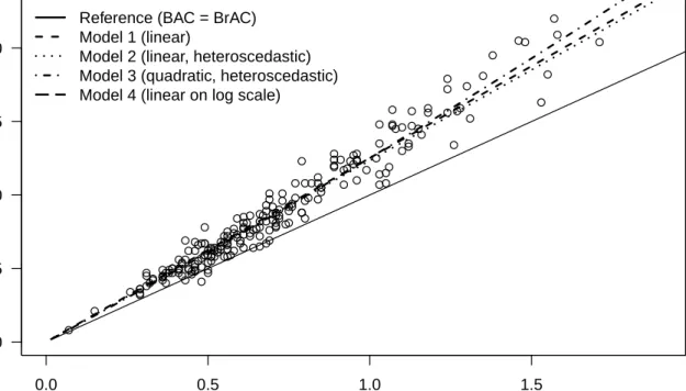
Both BAC and BrAC measurements of 212 persons were made available, where the BrAC measurements have been already transformed to BAK estimates based on the commonly used transformation factor 2000. A scatterplot of the original data is given in Figure 1. The models appearing in the plot are discussed below.
[Figure 1 about here.]
Figure 1 reveals that breath alcohol concentration tends to underestimate blood alcohol concentration. We fitted four linear regression models to these data in order to derive a suitable prediction model for BAC given BrAC. Note that the inclusion of further explanatory variables, such as gender or age is not of interest, as such information is not used in practice. All models are constructed such that the mean blood alcohol level is 0 if breath alcohol is 0. The fitted models were:
• Model 1: a simple linear model yi = γ1xi +ui without intercept, where yi and xi are
observed blood and breath alcohol concentration of individual i, γ1 is an unknown slope
parameter and ui is a mean-zero error term with variance τ2,
• Model 2: as model 1 but with heteroscedastic variance τ2
i =x2i of the error term.
• Model 3: as model 2, but with an additional quadratic term: yi =γ1xi+γ2x2i +ui.
• Model 4: a simple linear model for logyi with unknown intercept γ0 and offset logxi,
i.e. logyi =γ0+logxi+ui. The logarithmic transformation has been suggested by Labianca
and Simpson (1996). Note that if the error terms in Model 1 and 4 would equal zero, then
the two models are equivalent with γ0 = logγ1.
The models are fitted using (weighted) least squares. Note that, for purposes of prediction
in the model (Fuller, 1987). The estimated coefficients of the different models can be found in Table 2.
Point predictions for blood alcohol concentration can now easily be obtained from the fitted models. However, interval predictions are of major interest in the present context, in particular validity of the 95% prediction interval is central. Under an additional normality
assumption on the error term ui the predictive distribution can be computed based on
standard results for the general linear regression model (Weisberg, 1985). The resulting
t-distribution can be well approximated by a normal distribution due to the large number
of degrees of freedom (> 200). In Model 4 this implies that the predictive distribution for
log blood alcohol concentration is normal, hence the predictive distribution for blood alcohol concentration is log-normal.
A plot (not shown) of the prediction intervals for each model reveals that prediction intervals resulting from Model 1 are wider than those for the other two models for small values of BrAC and shorter for large values of BrAC. This already indicates a possible miscalibration of Model 1.
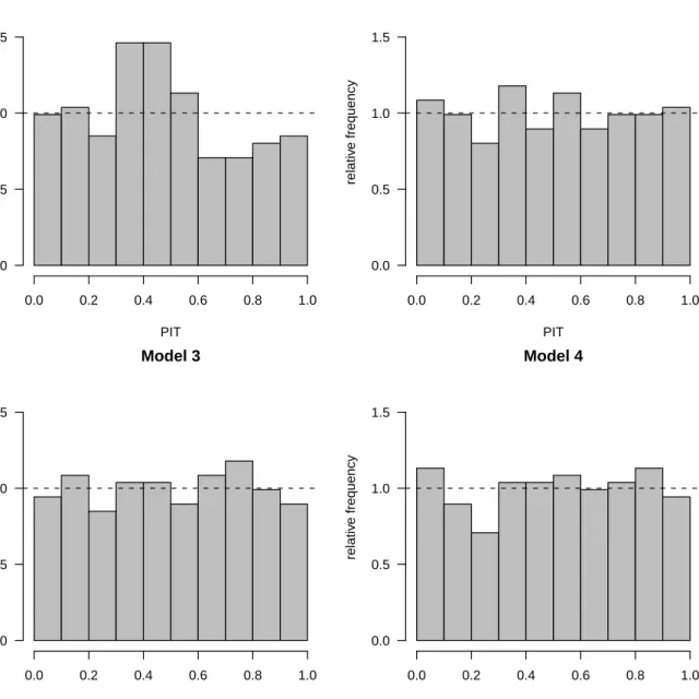
However, we would like to formally check how well ideally calibrated these models are for prediction. To this end, we perform a leave-one-out cross-validation to assess calibration of out-of-sample predictive distributions. Figure 2 displays the PIT histograms for the different
models. The p-values of a Kolmogorov-test on uniformity can be found in Table 2. There
is some indication that Model 1 is miscalibrated, but the evidence is not overwhelming (p
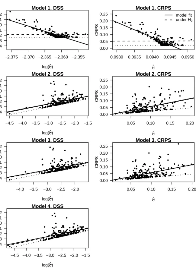
= 0.029). Based on the individual scores, we then applied the score regression approaches described in Section 4.2, i.e. computed the regression models (7) and (8) yielding least-squares
estimators ˆa,ˆbfor DSS and ˆc,dˆfor CRPS. The corresponding scatterplots of individual scores
can be found in Figure 3. Visual inspection indicates that Model 1 is strongly miscalibrated, with a tendency for increasing score values with decreasing (log) predictive standard
devi-ation. In a calibrated model, this should be the other way around. The other three models seem to be sufficiently well-calibrated.
[Figure 2 about here.] [Figure 3 about here.]
As for score regression, the resulting p-values for global χ2-tests of the hypotheses (9)
can be found in Table 2. The score regression approach clearly identifies Model 1 as not sufficiently calibrated and appears to have far more power than the Kolmogorov-test based
on the PIT values (very smallp-values in both cases). No evidence of miscalibration could be
found for the other three models, which also have very similar mean score values. Note that
CRPS and the corresponding CRP-score regression p-value is not available for log-normal
predictions (Model 4).
Finally, in Table 2 we also provide results of the deviance test for the cumulative exceedence probabilities, as introduced in Mason et al. (2007), not only for the median, but also for the
1st and 3rd quartile. This approach also shows no evidence of miscalibration of Model 3.
However, results for Models 1 and 2 are ambiguous. Note that contrary to score regression, the CEP approach has the disadvantage of introducing an additional parameter, the quantile
q(p) of interest, see (6). As a consequence, calibration test results for different quantiles may
differ, as in the current forensic application. See also the discussion in Section 4.1. It is therefore not clear what conclusion can be drawn from the CEP test regarding calibration of Models 1 and 2.
[Table 2 about here.]
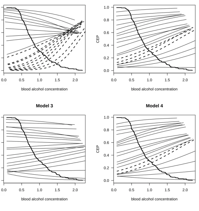
To gain further insight into the CEP approach, Figure 4 displays the estimated CEP curves for p= 0.05,0.1, . . . ,0.95 and the different models. The curves are useful for an explanatory assessment of calibration. In Model 1, all CEPs have very similar values for large values of
BAC. This is evidence of underdispersed predictions - regardless of the quantile q(p) - for large values of BAC. For small BAC values the predictions are overdispersed, the CEP curves cluster at the extremes values 0 and 1. Model 2 and especially Model 3 seem sufficiently better calibrated with approximately parallel CEP curves at evenly spaced heights.
[Figure 4 about here.]
6. Discussion
In this paper we have described new methodology for assessing calibration of continuous probabilistic predictions. In particular, a score regression approach based on scoring rules has proved to be useful. The method regresses individual scores on functions of the predictive variance, thus naturally complements the regression approach by Mason et al. (2007), where quantiles of the predictive distribution serve as covariates. However, note that the different tests assess different types of miscalibration. This is indicated in the results for Model 2, see Table 2. For this model, CEP identifies miscalibration for the third quartile, whereas according to the two score regression approaches no indication for miscalibration is found.
Initially we have focused on normal predictions, in which case analytic forms for the first two moments of the logarithmic and continuous ranked probability score could be derived for ideal forecasts. The unconditional tests can be applied for normal predictions, whereas the score regression approach can also be applied for certain non-normal predictions. Of course, the score regression approach depends crucially on variation of the individual predictive variances. If the predictive variance is constant for all predictions considered, the score regression approach will fail. The unconditional approach can then still be used in that case, if the predictive distribution is normal.
In two applications we have seen that the score regression approach has typically more power than other approaches considered. However, a general assessment of the power of any
of the proposed tests will require some assumptions about the data-generating distribution under the alternative. It is fairly easy to construct examples where the power of any of the tests described is low. For example, if the data-generating distribution is not fully determined by the first two moments, then the DSS-score regression approach may not be able to detect miscalibration if at least the first two moments of the forecast match the data-generating distribution. Even the unconditional tests may have poor power if the data-generating distribution is non-normal. In a small simulation study we found out the LS calibration test is not able to diagnose miscalibration of a normal forecast, if the true data-generating distribution has equal mean and variance, but is uniformly distributed. In this context we note that also the PIT values can be exactly uniform, although the forecast distribution may not equal the data-generating distribution such as for the climatological forecaster described in Section 5.1. Further research on the power of the different calibration tests seems warranted.
It is clear that in order to receive “good predictions” we should insist on having them calibrated. Calibration then serves as one (of possibly more) criteria for model selection, together with alternative measures such as AIC or BIC, or the mean score values of e.g. the CRPS. Understood this way, a significant result of one or more of the different calibration tests proposed in this paper does not immediately imply that a given set of predictions is not useful at all, calibration is only one aspect among others. Such an interpretation of calibration is frequently used in assessment of predictive performance of logistic regression models especially in the medical context, see e.g. Harrison et al. (2007) or Lix et al. (2008). An interesting research question is how to re-calibrate a miscalibrated model. This issue has been discussed for binary predictions resulting from logistic regression models via Cox (1958) calibration regression, see e.g. Steyerberg et al. (2004); Harrison et al. (2006). Further research is necessary into how to re-calibrate continuous predictions.
Furthermore, it is of interest how much the methods discussed here can be generalized to multivariate forecasts. Here the Box ordinate transform (Box, 1980; Gneiting et al., 2008) can be used as an alternative to PIT values. For multivariate normal predictions, the first two moments of the logarithmic score can be easily derived, and a score regression approach would be possible with the log predictive standard deviation replaced by the log determinant of the predictive covariance matrix. Score regression based on the energy score (Gneiting and Raftery, 2007), the multivariate analogue of the CRPS, is more difficult to employ. We are currently investigating calibration tests for multivariate forecasts in the context of longitudinal data analysis.
Acknowledgements
We thank Tilmann Gneiting for helpful discussions and Peter Iten for providing the data on alcohol concentration. We are also grateful for helpful comments by an Associate Editor and two referees on earlier versions of this paper.
References
Azzalini, A. and Capitano, A. (1999). Statistical applications of the multivariate skew normal
distribution. Journal of the Royal Statistical Society: Series B61, 579–602.
Box, G. (1980). Sampling and Bayes’ inference in scientific modelling and robustness.Journal
of the Royal Statistical Society: Series A (Statistics in Society) 143,383–425.
Brier, G. W. (1950). Verification of forecasts expressed in terms of probability. Monthly
Weather Review 78, 1–3.
Butler, R. W. (1986). Predictive likelihood inference with applications (with discussion). Journal of the Royal Statistical Society: Series B 48,1–38.
Cox, D. R. (1958). Two further applications of a model for binary regression. Biometrika
45, 562–565.
Czado, C., Gneiting, T., and Held, L. (2009). Predictive model assessment for count data. Biometrics to appear.
Dawid, A. P. (1982). The well-calibrated Bayesian. Journal of the American Statistical
Association 77, 605–610.
Dawid, A. P. (1984). Present position and potential developments: Some personal views.
Statistical theory. The prequential approach. Journal of the Royal Statistical Society:
Series A 174, 278–292.
Dawid, A. P. and Sebastiani, P. (1999). Coherent dispersion criteria for optimal experimental
design. Annals of Statistics 27, 65–81.
Fuller, W. A. (1987). Measurement Error Models. John Wiley & Sons, New York.
Gerds, T. A., Cai, T., and Schumacher, M. (2008). The performance of risk prediction
models. Biometrical Journal 50,457–479.
Gneiting, T., Balabdaoui, F., and Raftery, A. E. (2007). Probabilistic forecasts, calibration
and sharpness. Journal of the Royal Statistical Society, Series B 69,243–268.
Gneiting, T., Larson, K., Westrick, K., Genton, M. G., and Aldrich, E. (2006). Calibrated probabilistic forecasting at the Stateline wind energy center: The regime-switching
space-time method. Journal of the American Statistical Association 101, 968–979.
Gneiting, T. and Raftery, A. E. (2007). Strictly proper scoring rules, prediction, and
estimation. Journal of the American Statistical Association 102, 359–378.
Gneiting, T., Stanberry, L., Grimit, E., Held, L., and Johnson, N. (2008). Assessing proba-bilistic forecasts of multivariate quantities, with an application to ensemble predictions
of surface winds. Test 17, 211–235.
comparison of prognostic classification schemes for survival data. Statistics in Medicine
18, 2529–2545.
Hamill, T. (2001). Interpretation of rank histograms for veryfying ensemble forecasts. Monthly Weather Review 129, 550–560.
Harrison, D. A., Brady, A. R., Parry, G. J., Carpenter, J. R., and Rowan, K. (2006). Recalibration of risk prediction models in a large multicenter cohort of admissions to
adult, general critical care units in the United Kingdom. Critical Care Medicine 34,
1378–1388.
Harrison, D. A., Parry, G., Carpenter, J., Short, A., and Rowan, K. (2007). A new risk prediction model for critical care: The Intensive Care National Audit and Research Centre
(ICNARC) model. Critical Care Medicine 35, 1091–1098.
Hosmer, D. W. and Lemeshow, S. (1989). Applied Logistic Regression. John Wiley & Sons,
New York.
Labianca, D. A. and Simpson, G. (1996). Statistical analysis of blood- to breath-alcohol
ratio data in the logarithm-transformed and non-transformed modes. European Journal
of Clinical Chemistry and Clinical Biochemistry 34, 111–117.
Leone, F., Nelson, L. S., and Nottingham, R. B. (1961). The folded normal distribution. Technometrics 3,543–550. Correction in 22, 452.
Lix, L. M., Yogendran, M. S., Leslie, W. D., Shaw, S. Y., Baumgartner, R., Bowman, C., Metge, C., Gumel, A., Hux, J., and James, R. C. (2008). Using multiple data features improved the validity of osteoporosis case ascertainment from administrative databases. Journal of Clinical Epidemiology 61, 1250–1260.
Mason, S. J., Galpin, J. S., Goddard, L., Graham, N. E., and Rajartnam, B. (2007).
Conditional exceedance probabilities. Monthly Weather Review 135, 363–372.
regression models. Statistics in Medicine 10, 1213–1226.
Riebler, A. and Held, L. (2009). The analysis of heterogeneous time trends in multivariate
age-period-cohort models. Biostatistics
Sanders, F. (1963). On subjective probability forecasting. Journal of Applied Meteorology2,
191–201.
Schmid, C. H. and Griffith, J. L. (2005). Multivariate classification rules: Calibration and
discrimination. In Armitage, P. and Colton, T., editors, Encyclopedia of Biostatistics,
volume 5, pages 3491–3497. Wiley, 2nd edition.
Schumacher, M., Graf, E., and Gerds, T. (2003). How to assess prognostic models for survival
data: a case study in oncology. Methods of Information in Medicine 42,564–571.
Smith, J. Q. (1985). Diagnostic checks of non-standard time series models. Journal of
Forecasting 4, 283–291.
Spiegelhalter, D. (1986). Probabilistic prediction in patient management and clinical trials. Statistics in Medicine 5, 421–433.
StataCorp. (2003). STATA, reference A-F. Stata Corporation, 8.0 edition.
Steyerberg, E. W. (2009). Clinical Prediction Models. Springer, New York.
Steyerberg, E. W., Borsboom, G. J., van Houwelingen, H. C., Eijkemans, M. J., and Habbema, J. D. (2004). Validation and updating of predictive logistic regression models:
a study on sample size and shrinkage. Statistics in Medicine 23,2567–2586.
Appendix
The folded normal distribution
For a normally distributed random variable Z with mean µ and variance σ2, the random
variable Y =|Z| has a folded normal distribution with expectation
E(Y) = 2σϕ(µ/σ) +µ{2Φ(µ/σ)−1} (A.1)
and variance
Var(Y) = σ2 +µ2−E(|Z|)2,
see Leone et al. (1961). In the special case µ = 0, a so-called half-normal distribution is
obtained with mean E(Y) = σp2/π and variance Var(Y) = σ2(1−2/π).
Variance of the CRPS
Let Z =|Y1−Yobs|. To calculate the variance of the CRPS, we first note that
Var{CRPS(Yobs)} = Var E(Z|Yobs)
= Var(Z)−E Var(Z|Yobs). (A.2)
Under normality, the first term in (A.2) equals Var(Z) = 2σ2(1−2/π), due to the properties
of the half-normal distribution. As for the second term, let vµ,σ = E Var(Z|Yobs). Since
vµ,σ = σ2v0,1 for any µ ∈ R and σ > 0, we assume µ = 0 and σ = 1 in the following.
Then, abbreviating the expectation of a folded normal random variable with mean y ∈ R
and variance 1 as
ψ(y) = 2ϕ(y) +y{2Φ(y)−1}, (A.3)
(compare (A.1)), we get
v = v0,1 = E{E(Z2|Yobs)} −E{E2(Z|Yobs)}
= E(Z2)−E{E2(Z|Y
obs)}
= 2−E{ψ2(Y
Using (A.3), we thus have
E{ψ2(Y
obs)} = E[4ϕ2(Yobs) +Yobs2{2Φ(Yobs)−1}2+ 4Yobsϕ(Yobs)(2Φ(Yobs)−1)]
=: 4m1+m2+ 4m3. Now, m1 = Z ϕ3(x)dx = (2·31/2π)−1.
Using integration by parts twice, it turns out that m3 =m1. As for m2,
m2 = E[Yobs2{2Φ(Yobs)−1}2] = 2 ∞ Z 0 x2ϕ(x){2Φ(x)−1}2dx.
Inserting x2ϕ(x) = ϕ00(x) +ϕ(x) and again integrating by parts, one deduces
m2 = 4m1+ 1/3. Collecting all these results, we obtain in total
Var{CRPS(Yobs)} = 2σ2(1−2/π)−σ2{2−(12m1+ 1/3)} = σ2{1/3−4/π+ 12/(2π√3)} = σ2(1/3−4/π+√12/π) = σ2³1 3− 4−√12 π ´ ≈ 0.16275·σ2.
0.0 0.5 1.0 1.5 0.0 0.5 1.0 1.5 2.0
breath alcohol concentration
b
lood alcohol concentr
ation
Reference (BAC = BrAC) Model 1 (linear)
Model 2 (linear, heteroscedastic) Model 3 (quadratic, heteroscedastic) Model 4 (linear on log scale)
Figure 1. Scatterplots for blood vs. breath alcohol concentrations and fitted regression models.
0.0 0.2 0.4 0.6 0.8 1.0 0.0 0.5 1.0 1.5 Model 1 PIT relativ e frequency 0.0 0.2 0.4 0.6 0.8 1.0 0.0 0.5 1.0 1.5 Model 2 PIT relativ e frequency 0.0 0.2 0.4 0.6 0.8 1.0 0.0 0.5 1.0 1.5 Model 3 PIT relativ e frequency 0.0 0.2 0.4 0.6 0.8 1.0 0.0 0.5 1.0 1.5 Model 4 PIT relativ e frequency
−2.375 −2.370 −2.365 −2.360 −2.355 −4 −3 −2 −1 0 1 2 Model 1, DSS log(σ^) LS i 0.0930 0.0935 0.0940 0.0945 0.0950 0.00 0.05 0.10 0.15 0.20 0.25 Model 1, CRPS σ^ CRPS model fit under H0 −4.5 −4.0 −3.5 −3.0 −2.5 −2.0 −1.5 −4 −3 −2 −1 0 1 2 Model 2, DSS log(σ^) LS 0.05 0.10 0.15 0.20 0.00 0.05 0.10 0.15 0.20 0.25 Model 2, CRPS σ^ CRPS −4.0 −3.5 −3.0 −2.5 −2.0 −4 −3 −2 −1 0 1 2 Model 3, DSS log(σ^) LS 0.05 0.10 0.15 0.20 0.00 0.05 0.10 0.15 0.20 0.25 Model 3, CRPS σ^ CRPS −4.5 −4.0 −3.5 −3.0 −2.5 −2.0 −1.5 −4 −3 −2 −1 0 1 2 Model 4, DSS log(σ^) LS
Figure 3. Score regression plots. Shown are the individual scores (dots), a linear fit to the individual scores (solid), the expected value for ideal forecasts (dashed), and DSSmin and
CRPSmin (dotted), respectively. Note that in the lower three rows, the fitted and ideal lines
0.0 0.5 1.0 1.5 2.0 0.0 0.2 0.4 0.6 0.8 1.0 Model 1
blood alcohol concentration
CEP 0.0 0.5 1.0 1.5 2.0 0.0 0.2 0.4 0.6 0.8 1.0 Model 2
blood alcohol concentration
CEP 0.0 0.5 1.0 1.5 2.0 0.0 0.2 0.4 0.6 0.8 1.0 Model 3
blood alcohol concentration
CEP 0.0 0.5 1.0 1.5 2.0 0.0 0.2 0.4 0.6 0.8 1.0 Model 4
blood alcohol concentration
CEP
Figure 4. Estimated CEP curves forp= 0.05,0.1, . . . ,0.95 and the three different forensic models. The dotted curves denote slopes significantly different from zero with a significance level equal to 0.01, and the decreasing step function is 1 minus the empirical distribution function of the blood alcohol concentration sample.
Table 1
Proportion of rejected null hypotheses for Hamill’s forecast in 10000 simulations. n= 20 n= 50 n= 100 n= 500 n= 10000 n=100000
PIT Kolmogorov-test 0.038 0.044 0.044 0.048 0.094 0.729
LS calibration test 0.064 0.072 0.075 0.104 0.579 1.000
CRPS calibration test 0.048 0.050 0.049 0.060 0.280 0.992
CEP test median 0.107 0.142 0.220 0.760 1.000 1.000
DS-score regression 0.141 0.201 0.444 0.999 1.000 1.000
Table 2
Estimates from the different regression models, mean scores, andp-values of calibration tests.
Model 1 Model 2 Model 3 Model 4
effect x x x x2 1 ˆ γ 1.251 1.234 1.184 0.068 0.171 se(ˆγ) 0.008 0.009 0.022 0.027 0.009 ˆ δ 0.915 0.859 se(ˆδ) 0.116 0.114 DSS -1.860 -1.998 -2.007 -2.001 CRPS 0.052 0.050 0.049 NA
Kolmogorov-test PIT values 0.029 0.913 0.996 0.810
CEP test 0.25-quantile 0.117 0.115 0.615 0.0380
CEP test median 0.0113 0.0455 0.886 0.0613
CEP test 0.75-quantile 4.77e-07 0.000729 0.171 0.000726
DS-score regression <2e-16 0.941 0.937 0.702