DigitalCommons@University of Nebraska - Lincoln
Computer Science and Engineering: Theses,
Dissertations, and Student Research Computer Science and Engineering, Department of
8-2016
Exploring Dynamic Memory Allocations for
Bioinformatics Applications
Nitya Kovur
University of Nebraska-Lincoln, [email protected]
Follow this and additional works at:http://digitalcommons.unl.edu/computerscidiss
Part of theComputer Engineering Commons
This Article is brought to you for free and open access by the Computer Science and Engineering, Department of at DigitalCommons@University of Nebraska - Lincoln. It has been accepted for inclusion in Computer Science and Engineering: Theses, Dissertations, and Student Research by an authorized administrator of DigitalCommons@University of Nebraska - Lincoln.
Kovur, Nitya, "Exploring Dynamic Memory Allocations for Bioinformatics Applications" (2016).Computer Science and Engineering: Theses, Dissertations, and Student Research. 108.
APPLICATIONS
by
Nitya Kovur
A THESIS
Presented to the Faculty of
The Graduate College at the University of Nebraska
In Partial Fulfillment of Requirements
For the Degree of Master of Science
Major: Computer Science
Under the Supervision of Professor Jitender S Deogun
Lincoln, Nebraska
Nitya Kovur, M.S
University of Nebraska, 2016
Advisor: Jitender S Deogun
The progression of scientific data leads to an increase in the demand of powerful high performance computers (HPC) where data can be stored and analyzed. High performance computing is used in several research areas to solve large problems. How-ever, efficient usage of supercomputing resources that are available is a major concern for most of the researchers. The user has to choose the amount of resources needed for execution before submitting the job. Over or under subscription of resources leads to low system utilization and/or low user satisfaction.
Bioinformatics is one such field that heavily relies on HPC. One of the fundamental problems in bioinformatics is Genome Assembly. Generally, genome assembly tools require HPC systems with very large memories for the assembly process. Therefore, estimating the memory requirements of genome assembly tools prior to the assembly process is highly important.
We explore the methods to possibly predict the dynamic memory allocation for big data applications. Our approach for solving the problem is that, memory required by a specific type of application (e.g. genome assembly) can be predicted by execut-ing the application for small fractions of the dataset. In order to test our hypothesis, we have carried out experiments in three stages. First, we compare two resource monitoring tools in order to study effective memory consumption of the applications.
genome assembly applications (Velvet, Ray, and IDBA) on six different datasets. Furthermore, we investigate whether running the assembly on a small fraction of the data (process executable in a short time) can help us in predicting the memory and time resources required to assemble the full dataset. The generated results show that the memory usage obtained from different resource monitoring tools slightly differs for our datasets. Moreover, different fractions of data show similar patterns of mem-ory usage.
In stage 2, to further test our hypothesis, we analyzed the memory consumption of three different de novo genome assembly applications (Velvet, SPAdes, and Soap-DeNovo) on four different datasets. For each experiment we use three fractions of the dataset (10%, 20%, and 30%) and record the memory usage over time. Knowing this, we are able to build a linear model that can predict the memory usage of the entire dataset based on the dataset size. Using this model, we predict the memory usage of the full datasets with 2.582%, 19.29%, 9.62% and 43.55% error rates for Velvet, 4.506%, 27%, 55.11% and 173% error rates for SPAdes and 3.353%, 68%, 32% and 20.77% error rates for SoapDeNovo for dataset1, dataset2, dataset3 and dataset4 respectively.
In stage 3, we analyzed the memory usage for three different de novo genome as-sembly applications (Velvet, SoapDeNovo, Spades) on three different input datasets. For each experiment we use six fractions of the dataset (1%, 2%, 3%, 10%, 20%, 30%) and record the memory usage over time. Next, we use seven different machine learn-ing techniques (k-Nearest Neighbor, Linear Regression, Multivariate Adaptive Re-gression Splines, Neural Networks, Principal Component ReRe-gression, Stepwise Linear Regression and Support Vector Machines) to build the prediction model. The linear
9.62% error rates for Velvet; 3.353%, 68% and 32% for SoapDeNovo, and 4.506%, 27% and 68% error rates for Spades for input Dataset1, Dataset2 and Dataset3 re-spectively.
Considering that for a given input dataset and an application, the data fractions used have similar peak memory distributions, we believe that building a model for dynamic memory prediction and allocation is may be realistic and feasible.
ACKNOWLEDGMENTS
I am using this opportunity to express my gratitude to everyone who supported me throughout the course of my Masters program. I am thankful for their aspiring guid-ance, invaluably constructive criticism and friendy advices.
Firstly, I am extremely grateful to my advisor Dr. Jitender Deogun for his constant support during my M.S study and research. His motivation and immense knowledge in the subject helped me all the time during my research. I could not have imagined having a better mentor for my M.S. The door to Dr. Deoguns office was always open whenever I ran into a trouble spot or had a question about my research or writing.
I would like to thank the rest of my thesis committee: Dr. Byrav Ramamurthy and Dr. David Swanson, for their precious time, considerate and critical reading of this thesis.
I would also like to thank Natasha Pavlovikj for helping me with this research. I am gratefully indebted to her for her very valuable comments on this thesis.
Finally, I must express my very profound gratitude to my parents and to my hus-band for providing me with unfailing support and continuous encouragement through-out my years of study and through the process of researching and writing this thesis. This accomplishment would not have been possible without them. Thank you.
TABLE OF CONTENTS
CHAPTER 1 ... 1
Introduction ... 1
1.1 Background ... 1
1.2 Scope of the research ... 2
1.3 Outline of chapters ... 3
CHAPTER 2 ... 5
GENOME ASSEMBLY APPLICATIONS ... 5
2.1 Velvet ... 5
2.2 Ray ... 6
2.3 IDBA... 6
2.4 SPAdes ... 6
CHAPTER 3 ... 8
MEMORY TRACKING TOOLS... 8
3.1 Resource Monitor ... 9
3.2 Cgroup Monitor ... 10
CHAPTER 4 ... 11
EXPERIMENTAL SETUP STAGE 1... 11
4.1 Experimental Data ... 13
4.2 Experimental Results and Evaluation ... 13
4.2.1 Resource Monitor vs Cgroup Monitor ... 13
4.2.2 Comparison of the Plots Generated ... 18
CHAPTER 5 ... 21
EXPERIMENTAL SETUP STAGE 2 ... 21
5.1 Experimental Data ... 21
5.2.1 Generating Linear Models for Velvet, SPAdes and SoapDeNovo ... 22
5.2.2 Predicted Memory Percentage Error ... 27
CHAPTER 6 ... 30
EXPERIMENTAL SETUP STAGE 3 ... 30
6.1 Machine Learning Techniques ... 30
6.1.1 k-Nearest Neighbor ... 31
6.1.2 Linear Regression ... 32
6.1.3 Multivariate Adaptive Regression Splines ... 33
6.1.4 Neural Networks ... 33
6.1.5 Principal Component Regression ... 34
6.1.6 Stepwise Linear Regression ... 34
6.1.7 Support Vector Machines ... 35
6.3 Experimental Results and Evaluation ... 38
6.3.1 Comparing Memory Prediction Error Rates for Multiple Machine Learning Techniques ... 38
6.3.2 Evaluation of Memory Prediction Models using Regression Metrics .. 41
6.3.2.1 RMSE ... 42
6.3.2.2 MAPE ... 43
CHAPTER 7 ... 46
DISCUSSIONS AND CONCLUSIONS ... 46
7.1 Summary of Results ... 46
7.2 Limitations and Future Scope ... 49
LIST OF TABLES
Table 4.1: Description of the NGS data used in the experiments ... 12
Table 4.2: Total running time and maximum memory consumed using cgroup moni-tor ... 19
Table 4.3: Total running time and maximum memory consumed using resource mon-itor ... 20
Table 5.1: Overall characteristics of the datasets used ... 22
Table 6.1: Overall characteristics of the datasets used ... 37
Table 6.2: Coloring scheme on Machine Learning Techniques used in the experiments ... 45
LIST OF FIGURES
Figure 4.1: Velvet, Ray, and IDBA memory consumption of 10, 50, 100 percent of the input Dataset 1 respectively ... 14
Figure 4.2: Velvet, Ray, and IDBA memory consumption of 10, 50, 100 percent of the input Dataset 2 respectively ... 14
Figure 4.3: Velvet, Ray, and IDBA memory consumption of 10, 50, 100 percent of the input Dataset 3 respectively ... 14
Figure 4.4: Velvet, Ray, and IDBA memory consumption of 10, 50, 100 percent of the input Dataset 4 respectively ... 15
Figure 4.5: Velvet, Ray, and IDBA memory consumption of 10, 50, 100 percent of the input Dataset 5 respectively ... 15
Figure 4.6: Velvet, Ray, and IDBA memory consumption of 10, 50, 100 percent of the input Dataset 6 respectively ... ... 15
Figure 4.7: Velvet, Ray, and IDBA memory consumption using resource monitor and cgroup monitoring with Dataset 1 ... 16
Figure 4.8: Velvet, Ray, and IDBA memory consumption using resource monitor and cgroup monitoring with Dataset 2 ... 16
cgroup monitoring with Dataset 3 ... 16
Figure 4.10: Velvet, Ray, and IDBA memory consumption using resource monitor and cgroup monitoring with Dataset 4 ... 17
Figure 4.11: Velvet, Ray, and IDBA memory consumption using resource monitor and cgroup monitoring with Dataset 5 ... 17
Figure 4.12: Velvet, Ray, and IDBA memory consumption using resource monitor and cgroup monitoring with Dataset 6 ... 17
Figure 5.1: Linear equations for Velvet and dataset1, dataset2, dataset3, dataset4 based on the peak memory consumed per dataset fraction size ... 24
Figure 5.2: Linear equations for SPAdes and dataset1, dataset2, dataset3, dataset4 based on the peak memory consumed per dataset fraction size ... 25
Figure 5.3: Linear equations for SoapDeNovo and dataset1, dataset2, dataset3, dataset4 based on the peak memory consumed per dataset fraction size ... 25
Figure 5.4: Predicted memory percentage error rates for Velvet, SPAdes and Soap-DeNovo for dataset1, dataset2, dataset3 and dataset4 ... 28
Figure 6.1: Comparison of the predicted memory for kNN, when k is 1, 2, 3, 4, 5 and 6 respectively ... 32
Figure 6.2: Error rates of memory prediction models generated from multiple ma-chine learning techniques ... 36
Figure 6.3: Comparison of multiple models using the RMSE regression metrics ... 39
CHAPTER 1
INTRODUCTION
1.1 Background
Due to an immense expansion of scientific data, there is a constant increase in the demand of powerful computational resources. For big data to be stored and analyzed, the use of High Performance Computers (HPC) is inevitable. The HPC systems are expensive and constantly evolving. Moreover, these systems are shared among vari-ous users.
A high performance computer, can be used and managed without a lot of expense or expertise. Therefore, HPC users include scientists from various disciplines, such as biology, chemistry, physics, earth sciences and astronomy. Primary goal of these users is to obtain desired computational results. However, as discussed earlier, they do not have enough expertise to optimize their programs to reduce computational resource requirements including execution time. Also, non-computer science users might not be interested in considering various HPC software and hardware utilizations. These constraints lead to lower utilization of resources and reduced user satisfaction.
Various tools are available that can help us to effectively utilize the HPC systems. Resources commonly tracked by these tools include: CPU cores, memory usage, wall time and file size. All of these tools are designed to collect resource usage data as the programs are executed. Also, focus of these tools is on overall system utilization and not on resource usage per program/job. Several previous studies use machine learning algorithms to predict the resource requirements of an application. Most of these
pre-dictions are based on historical information of the application resource consumption in order to predict the application run time. However, no such mechanism is available that can dynamically predict the resource requirement of the job prior to its execution.
Among many disciplines, bioinformatics is one such area which highly relies on the use of HPC. Genome assembly is one of the fundamental problems in bioinformatics. Therefore, we have chosen genome assembly applications as high-performance scien-tific applications to analyze the memory usage and utilization of HPC. The input for genome assembly is generated using next-generation sequencing (NGS) technologies. NGS technologies produce large amount of fragmented genome reads that need to be assembled. As of August 2014, GenBank, the central repository of genetic se-quence information hosted by the NCBI, contains 16.6 billion bases from 175 million reported sequences. This number is constantly growing. These fragmented genome reads require HPC systems with very large memories for the assembly process. For example, assembling a genome of 250 MB requires more than 256 GB RAM. Even though there are existing parallel implementations of various genome assemblers, the main focus of these tools is the assembly quality, not the HPC resource utilization.
1.2 Scope of Research
Goal of our research was to find mechanisms to dynamically predict the resource utilization for big data applications. For this purpose, we have divided our research into two stages.
In the first stage, we run experiments and present a preliminary analysis of re-sources consumed by three commonly used genome assembly tools, Velvet [10], Ray [7] and IDBA [9] over six different datasets. The resources considered are memory
and time. Memory usage is tracked using two resource monitoring approaches using resource monitor [1] and cgroup Linux container [2]. From the results obtained, we observed that memory usage by different resource monitoring tools slightly differs for our datasets. Also, we found similar patterns of memory usage for different fractions of data. Based on the results of our first stage, we found that the memory required by an application can be predicted by executing the application for small fractions of the dataset.
In order to test our hypothesis, in the second stage, we investigate the memory usage of three genome assembly applications, Velvet, SPAdes and SoapDeNovo. We track the memory usage for small fractions of the dataset (10%, 20%, 30%) using resource monitor, a tool for monitoring HPC resources. Using the memory tracked, we try to develop linear regression equations to predict memory usage for 100% of data. This will be the predicted value. We also run experiments to track the memory usage when 100% of dataset is used. This will be the actual value of memory used. We then calculate the error rate based on predicted and actual values of memory used.
In the third stage, we track the memory consumed by few applications when the applications are run with small fractions of the entire input dataset (1%, 2%, 3%, 10%, 20%, 30%). For this purpose, we used seven machine learning techniques (k-Nearest Neighbor, Linear Regression, Multivariate Adaptive Regression Splines, Neural Networks, Principal Component Regression, Stepwise Linear Regression and Support Vector Machines) in order to build model for memory prediction. Knowing the sizes of the smaller dataset fractions and the consumed memory, we expect that the memory consumed depends on the size of the input dataset. We also believe that the Size Memory relationship should be linear. However, to test this, we include machine learning techniques that consider both linear and non-linear associations.
Our main objective is to use this information to build a model for dynamic re-source estimation for various big data applications.
1.3 Outline of chapters
The thesis is presented in the following chapters. Chapter 2 provides an insight into the Genome assembly tools use for the research. Chapter 3 describes the memory tracking tools used. Chapter 4, 5, 6 presents the experimental setup, results and eval-uation for stages 1,2, and 3 respectively. Chapter 7 summarizes the major findings of this research. The limitations and future work of this study are also presented in this chapter.
CHAPTER 2
GENOME ASSEMBLY APPLICATIONS
In bioinformatics, sequence assembly refers to the process of aligning and merging fragments of a long DNA sequence so as to rebuild the original sequence. With the recent and rapid development of next-generation sequencing, the genome sequence data is produced faster, easier, and more accurately [9]. The need to assemble this data led to development of various de novo assembly tools. De novo sequencing, is a technique in which sequencing analysis is performed without the aid of a reference genome. The main approach behind these tools uses de Bruijn graphs and k-mers. Examples include Euler [1], AbySS [1], SOAPdenovo [1] and Velvet [9]. Although efficient, de Bruijn graph construction is highly memory consuming for mostly all traditional genome assemblers.
2.1 Velvet
Velvet [9] is one of the most widely used de novo genomic assembler, specially designed for short read sequencing technologies. This is achieved by manipulating the de Bruijn graphs for genomic sequence assembly by removing errors and the sim-plifying repeated regions. It builds de Bruijn graphs from the sequenced reads and produces the best assembly. This process happens in two steps: hashing and graph building. The hashing process is composed of building a dictionary of all words of length k. The second process uses the dictionary to build de Bruijn graph from the words of length k and find Eulerian paths afterwards. These steps correspond to two Velvet executables, velveth and velvetg respectively [9].
2.2 Ray
Ray [14] is a parallel software that generates de novo genome assemblies with next-generation sequencing data. Ray makes use of a de Bruijn graphs. However, instead of using Eulerian paths, this approach uses specific subsequences, called seeds. These seeds are further extended into contigs. Ray is scalable tool because it uses message passing interface. This algorithm is run with only one executable, Ray.
2.3 IDBA
IDBA [15] is practical iterative de Bruijn graph de novo assembler for genome assembly. For the various de Bruijn graph approaches, the crucial part is to find a specific value of k. IDBA uses not only the specified k value, but also a range of k values to build the de Bruijn graph. IDBA is fast, parallel and convenient for assem-bling large scale genome assembly. The new version of IDBA, IDBA-UD performs better than the standard version and is executed with one executable, idba-ud.
2.4 SPAdes
SPAdes is a genome assembler, initially designed for single-cell and multi-cell bac-terial data. It breaks data into fixed-size words of length k to build the de Bruijn graph. The values of k are selected automatically based on the read length and data type. In the next stage, errors are detected and removed and paths through the graph are found. These paths are the contigs that belong to the final assembly. SPAdes main executable script is spades.py. This script includes modules for read-error correction, assembly, mismatch correction, alignment and assembly for highly polymorphic diploid genomes.
2.5 SoapDeNovo
SoapDeNovo is a de novo assembler for short reads. It is both memory and time efficient and it can be used for assembling large genomes such as the human genome. SoapDeNovo is composed of six modules: read-error correction, construction of de Bruijn graph, contig assembly, mapping of paired-end reads, scaffold construction and gap closure. The de Bruijn graph is built of data fragments of odd length k. SoapDeNovo requires a configuration file and an executable SOAPdenovo-63mer. The configuration file contains relevant information about the data and libraries used.
CHAPTER 3
MEMORY TRACKING TOOLS
With the constant development of HPC systems and high- performance scientific ap-plications, effective resource monitoring tools are expected for system profiling. With-out these tools, system resources can be easily underutilized (resulting in wasted/unused resources) or oversubscribed (resulting in failures/slow execution). While most of the resource monitoring tools collect statistics on system-level, there are a few that col-lect statistics on job-level. Some of the open source and commercial resource usage monitoring tools include: Gangila [17], systat/SAR [17], iostat [17]. Kickstart [2] is part of the Pegasus Workflow Management Systems and monitors HTC tasks. The TACC Stats package is a resource usage monitoring tool for HPC systems [17]. One of the best ways to expose memory usage and limits inside Linux containers [17] is to consider the metrics included in the control group, cgroup. This tool is powerful in controlling the amount of memory CPU, disk I/O or network I/O each process or user can actually use. However, most of the current system resource monitoring metrics were created before cgroup (free, top, vmstat) and they read metrics from the proc filesystem [1]. The proc filesystem is not containerized, meaning that the memory values they record come from the host system as a whole, not from the limits imposed by the cgroup. This means that the memory recorded from the proc filesystem does not usually represent the actual memory consumed from our program. Therefore, sometimes when our program fails due to exceeded memory limits, using free/top still shows less consumed memory than the one we are asking for. Considering this, tracking the memory usage from the cgroup container should help us gather the actual memory usage for our job. However, the cgroup container is private and we have not found a monitoring tool that can read information inside containers from system level.
For the purpose of our research, we use two resource monitoring tools:
1. resource monitor: uses the procfs Linux filesystem to obtain the statistics for the observed resource.
2. cgroup monitor: a custom script written to read the memory usage directly from the cgroup of the program process.
Both resource and cgroup monitor are executed from user level, as a wrapper to the program the user runs.
3.1 Resource Monitor
Resource monitor is a tool that monitors the computational resources used by a process. The data from resource monitor is gathered from procfs on Linux, and the kernel kvm interface on FreeBSD. The information about CPU usage, user and system time, and peak resident memory size is obtained using the getrusage() system call. However, in this approach, periodically short running processes can be missed. Resource monitor measures peak resource usage value while the task is running, be-cause this information is not available once the program terminates.
Resource monitor generates three report files:
1. a summary file with the maximum values of resources used.
2. a time-series that shows the resources used at periodic time intervals. 3. a list of files that were open (read and write) during execution.
Also, when a program is terminated due to exceeding resource limits, resource mon-itor reports the resources that went over the respective limits. Moreover, resource
monitor wraps some libc functions for better estimate of the resources used. It can monitor only the root process or its children as well.
3.2 Cgroup Monitor
Cgroup monitor is a simple tool we created to track the memory usage per time for a given process. Unlike the current monitoring tools, with cgroup monitor we gather data directly from the cgroup container. This method focuses on monitoring the cgroup resources from user perspective and uses the users privileges rather than those available to the system administrators. This means the user executes cgroup monitor together with the program that is monitored. Although this approach is experimental and further data smoothing and normalization is required, it is interesting to compare cgroup monitor tool with the other resource monitoring methods.
Cgroup monitor generates one report file that contains the memory consumed over certain period of time.
CHAPTER 4
EXPERIMENTAL SETUP STAGE 1
The main objective of this stage is to compare the resources (memory and time) tracked by two different resource monitoring methods when three different genome assembly tools are used. For Velvet, Ray and IDBA we use both resource monitor and cgroup monitor to compare the used memory and observe whether this value varies. Furthermore, we observe the memory usage when the genome assembly tools are run on the full dataset (100% dataset) and smaller fractions (10% dataset, 50% dataset) of it. Based on this knowledge, we further investigate whether running the whole assembly on a smaller part of the data (process executable in short time) can help us build a model for dynamic resource estimation for various big data applications.
All experiments are conducted on Tusker, one of the HPC clusters managed by Holland Computing Center (HCC), a High Performance Computing provider for the University of Nebraska [18].
While cgroup monitor tool is a simple script created for the purpose of this re-search, resource monitor is part of the cctools package developed by The Cooperative Computing Lab from the University of Notre Dame. This package is under constant development, and we used resource monitor Stable Version 4.3.3.
Velvet, Ray and IDBA are genome assembly tools that are available on Tusker. In order to use them, we loaded their modules and created simple SLURM submit files.
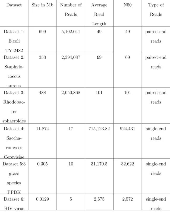
Dataset Size in Mb Number of Reads Average Read Length N50 Type of Reads Dataset 1: E.coli TY-2482 699 5,102,041 49 49 paired-end reads Dataset 2: Staphylo-coccus aureus 353 2,394,087 69 69 paired-end reads Dataset 3: Rhodobac-ter sphaeroides 488 2,050,868 101 101 paired-end reads Dataset 4: Saccha-romyces Cerevisiae 11.874 17 715,123.82 924,431 single-end reads Dataset 5:3 grass species PPDK 0.305 10 31,170.5 32,622 single-end reads Dataset 6: HIV virus 0.0129 5 2,575 2,572 single-end reads
4.1 Experimental Data
We used six DNA datasets from different organisms. Table 4.1 summarizes the details of each dataset, including its size, number of reads, length of reads, and read direction as well. Having datasets from different organisms and different sizes will help us observe the behavior of the genome assembly tools, and the resource usage.
4.2 Experimental Results and Evaluation
4.2.1 Resource Monitor vs. Cgroup Monitor for Genome Assembly Tools
The memory usage of three genome assembly tools is tracked using resource mon-itor and cgroup monmon-itor. Performing this experiment, we observe the difference of reported metrics when approaches using procfs and cgroup container are used respec-tively.
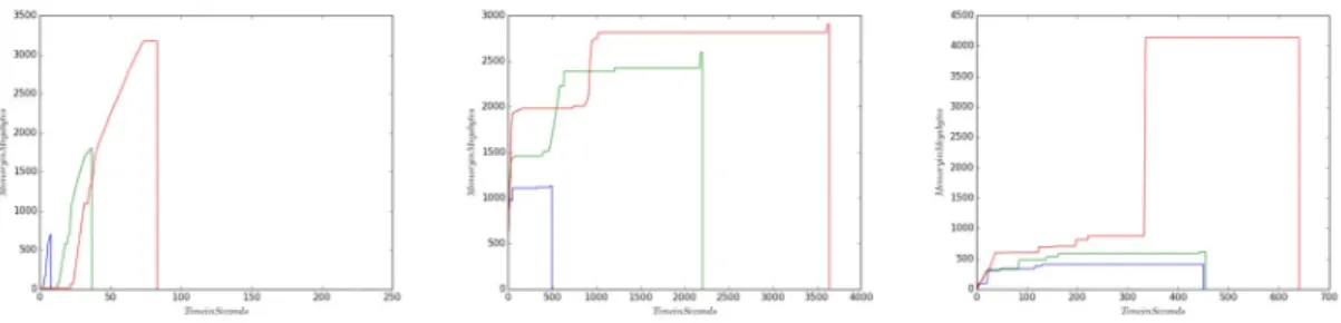
Figure 4.7-4.12 show the memory usage per time for Velvet, Ray and IDBA with the six different datasets. The xaxis is time in seconds, while the yaxis is -memory in MB. The blue line represents the values gathered from resource monitor, while the green line represents the values collected from cgroup monitor. We can see that the memory usage generated from cgroup monitor has similar curve as the mem-ory generated from resource monitor, but it is almost always higher. This difference can be observed from Table 4.2 and Table 4.3 respectively. The cgroup results are higher by about 2 GB for Velvet and Ray and by about 1.5 GB for IDBA.
Considering the running time, we can notice that even though we are using 3 genome assembly tools based on similar algorithms, their running time differs a lot.
The lowest running time is observed for Velvet, while the longest running time is produced when Ray is used.
Figure 4.1. Velvet, Ray, and IDBA memory consumption of 10, 50, 100 percent of the input Dataset 1 respectively.
Figure 4.2. Velvet, Ray, and IDBA memory consumption of 10, 50, 100 percent of the input Dataset 2 respectively.
Figure 4.3. Velvet, Ray, and IDBA memory consumption of 10, 50, 100 percent of the input Dataset 3 respectively.
Figure 4.4. Velvet, Ray, and IDBA memory consumption of 10, 50, 100 percent of the input Dataset 4 respectively.
Figure 4.5. Velvet, Ray, and IDBA memory consumption of 10, 50, 100 percent of the input Dataset 5 respectively.
Figure 4.6. Velvet, Ray, and IDBA memory consumption of 10, 50, 100 percent of the input Dataset 6 respectively.
Figure 4.7. Velvet, Ray, and IDBA memory consumption using resource monitor and cgroup monitoring with Dataset 1.
Figure 4.8. Velvet, Ray, and IDBA memory consumption using resource monitor and cgroup monitoring with Dataset 2.
Figure 4.9. Velvet, Ray, and IDBA memory consumption using resource monitor and cgroup monitoring with Dataset 3.
Figure 4.10. Velvet, Ray, and IDBA memory consumption using resource monitor and cgroup monitoring with Dataset 4.
Figure 4.11. Velvet, Ray, and IDBA memory consumption using resource monitor and cgroup monitoring with Dataset 5.
Figure 4.12. Velvet, Ray, and IDBA memory consumption using resource monitor and cgroup monitoring with Dataset 6.
4.2.2 Comparison of Plots Generated
For the next part of the experiments, we want to investigate whether running the assembly on a smaller part of the data (process executable in a short time) can help us predict the memory and time resources required to assemble the full dataset. Therefore, we run the three assembly tools and track the memory usage for 10%, 50% and 100% of the dataset.
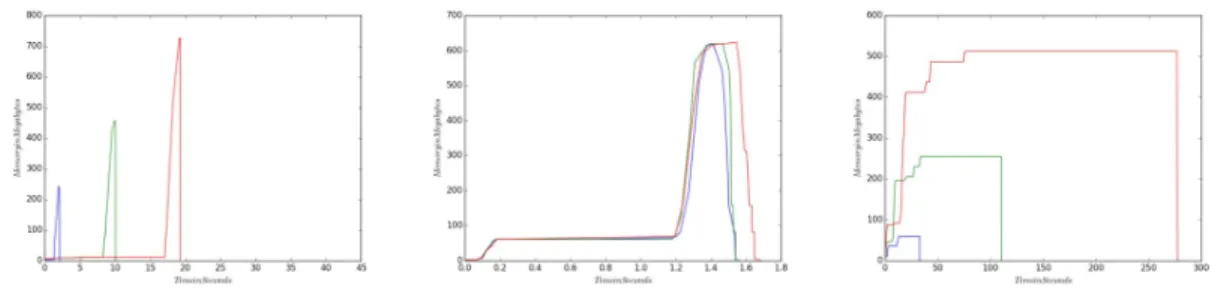
The obtained results are shown onFigure 4.1-4.6. The x-axis is time in seconds, while the y-axis is memory in MB. The blue line shows the memory usage for 10% of the full dataset. The green line is the memory consumption for 50% of the dataset, while the red line shows the memory usage for 100% of the dataset.
From these Figures, we can observe that the memory usage distribution for all three fractions of data follows a similar curve for all three assembly tools. Accordingly, the runs for 10% of the full dataset are much shorter compared to the runs for 100% of the dataset. Although Velvet, Ray and IDBA have different memory distributions for different datasets, all fractions ran for Velvet, Ray and IDBA are similar within the used tool.
Considering the shorter running time for smaller dataset, and the similar pattern of memory usage for different fractions of the initial data, we can say that building a model for dynamic resource allocation from these results is possible.
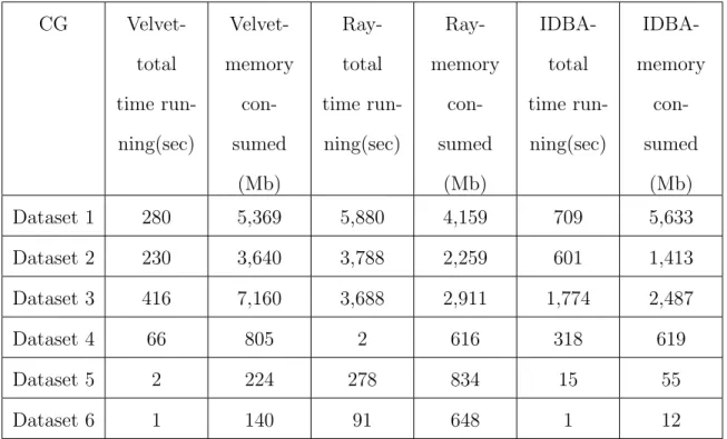
CG Velvet-total time run-ning(sec) Velvet-memory con-sumed (Mb) Ray-total time run-ning(sec) Ray-memory con-sumed (Mb) IDBA-total time run-ning(sec) IDBA-memory con-sumed (Mb) Dataset 1 280 5,369 5,880 4,159 709 5,633 Dataset 2 230 3,640 3,788 2,259 601 1,413 Dataset 3 416 7,160 3,688 2,911 1,774 2,487 Dataset 4 66 805 2 616 318 619 Dataset 5 2 224 278 834 15 55 Dataset 6 1 140 91 648 1 12
Table 4.2. Total running time and maximum memory consumed when cgroup monitoring is used.
RM Velvet-total time run-ning(sec) Velvet-memory con-sumed (Mb) Ray-total time run-ning(sec) Ray-memory con-sumed (Mb) IDBA-total time run-ning(sec) IDBA-memory con-sumed (Mb) Dataset 1 226 3,169 3,643 4,205 640 4,173 Dataset 2 202 3,271 2,264 1,739 662 1,192 Dataset 3 93 5,069 3,215 2,247 1,475 1,780 Dataset 4 43 728 2 610 277 519 Dataset 5 21 218 176 835 34 41 Dataset 6 11 137 92 640 24 6
Table 4.3. Total running time and maximum memory consumed when resoure monitor is used.
CHAPTER 5
EXPERIMENTAL SETUP STAGE 2
To generate data for this stage, four different datasets specified inTable 5.1 are used to run three popular bioinformatics applications. For each experiment, we track the memory usage when these applications are run on smaller fractions (e.g. 10%, 20%, 30%) of the full datasets. Based on this knowledge, we want to see whether running an application on a smaller data fraction (process executable in short time) can help us build a model for dynamic resource estimation for various big data applications.
For the purpose, we perform analysis for three popular bioinformatics applica-tions for generating genome assembly, Velvet, SPAdes and SoapDeNovo, on four DNA datasets from different organisms.
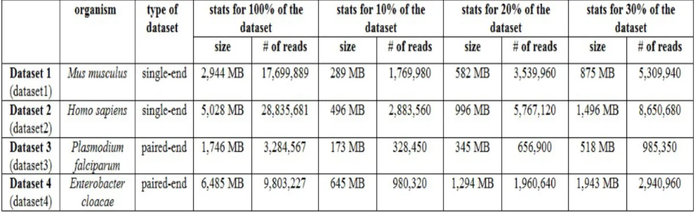
5.1 Experimental Data
Table 5.1 summarizes the details for each dataset, including its size and number of reads. We use two datasets with single-end reads with sizes of 2,944 MB and 5,028 MB respectively. We also use two datasets with paired-end reads with sizes of 1,746 MB and 6,485 MB.
The memory usage of the three genome assembly applications is tracked using resource monitor, tool for monitoring HPC resources.
Table 5.1. Overall characteristics of the datasets used.
5.2 Experimental Results and Evaluation
As part of the experiments, we initially used dataset fractions that represent 1%, 2% and 3% of the full dataset. However, the generated results produced unaccept-able error rates for predicting the memory resources used for the entire dataset. We observed similar behavior when 5%, 10% and 15% of the full dataset were used. How-ever, experiments for 10%, 20% and 30% of the dataset produced good error rates.
5.2.1 Generating Linear Models for Velvet, SPAdes and SoapDeNovo
For the first part of the experiment, we investigate whether running the genome assembly applications on a smaller data fraction can help us predict the memory re-sources required to assemble the entire dataset. For that reason, we extracted 10%, 20% and 30% of dataset1, dataset2, dataset3 and dataset4 respectively. The size and the number of reads of these dataset fractions are shown in Table 5.1. Next, we run Velvet, SPAdes and SoapDeNovo and track the memory usage for the various percentages of the datasets.
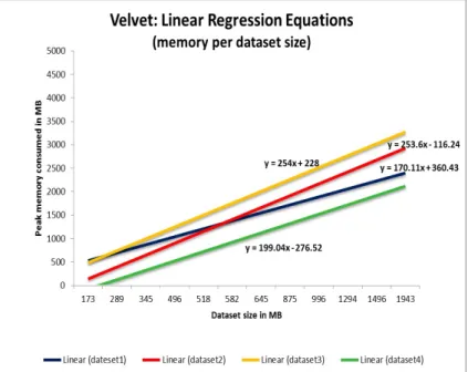
Figure 5.1 shows the experimental results when Velvet is used on 10%, 20% and 30% of dataset1, dataset2, dataset3 and dataset4 respectively. The x-axis rep-resents the dataset size in MBs, while the y-axis is the peak memory consumed in MBs. For example, for Velvet, for 10% of dataset1 (dataset size of 289 MB) the genome assembly reached peak memory of 738 MB; for 20% of dataset1 (dataset size of 582 MB) the peak memory is 1,269 MB; for 30% of dataset1 (dataset size of 875 MB) the recorded peak memory is 1,796 MB. Considering the peak memory values consumed for dataset1, we can observe that the memory linearly increases with the dataset size (blue line). Based on this, we are able to generate linear model for this dataset. The linear equation for dataset1 is y=170.11x+360.43, where x is the dataset size, and y is the peak memory. When we substitute x with the size of the entire dataset1 (2,944 MB) in the equation, y (the peak memory predicted) is 5,532.282 MB. Similarly, linear patterns are observed and models are generated for dataset2 (red line, y=253.6x-116.24), dataset3 (yellow line, y=254x+228) and dataset4 (green line, 199.04x-276.52).
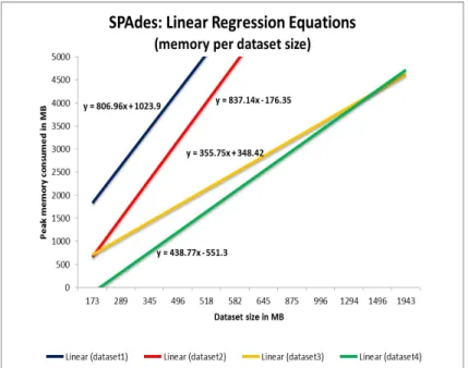
Figure 5.2 shows the experimental results when SPAdes is used on 10%, 20% and 30% of dataset1, dataset2, dataset3 and dataset4 respectively. The x-axis rep-resents the dataset size in MBs, while the y-axis is the peak memory consumed in MBs. For example, for SPAdes, for 10% of dataset1 (dataset size of 289 MB) the genome assembly reached peak memory of 2,865 MB; for 20% of dataset1 (dataset size of 582 MB) the peak memory is 5,184 MB; for 30% of dataset1 (dataset size of 875 MB) the recorded peak memory is 7,934 MB. Considering the peak memory values consumed for dataset1, we can observe that the memory linearly increases with the dataset size (blue line). Based on this, we are able to generate linear model for this dataset. The linear equation for dataset1 is y=806.96x+1023.9, where x is the dataset size, and y is the peak memory. When we substitute x with the size of
the entire dataset1 (2,944 MB) in the equation, y (the peak memory predicted) is 25,759.46 MB. Similarly, linear patterns are observed and models are generated for dataset2 (red line, y=837.14x-176.35), dataset3 (yellow line, y=355.75x+348.42) and dataset4 (green line, 438.77x-551.3).
Figure 5.1. Linear equations for Velvet and dataset1, dataset2, dataset3, dataset4 based on the peak memory consumed per dataset fraction size.
Figure 5.2. Linear equations for SPAdes and dataset1, dataset2, dataset3, dataset4 based on the peak memory consumed per dataset fraction size.
Figure 5.3. Linear equations for SoapDeNovo and dataset1, dataset2, dataset3, dataset4 based on the peak memory consumed per dataset fraction size.
Figure 5.3 shows the experimental results when SoapDeNovo is used on 10%, 20% and 30% of dataset1, dataset2, dataset3 and dataset4 respectively. The x-axis represents the dataset size in MBs, while the y-axis is the peak memory consumed in MBs. For example, for SoapDeNovo, for 10% of dataset1 (dataset size of 289 MB) the genome assembly reached peak memory of 1,882 MB; for 20% of dataset1 (dataset size of 582 MB) the peak memory is 2,171 MB; for 30% of the dataset1 (dataset size of 875 MB) the recorded peak memory is 2,505 MB. Considering the peak memory values consumed for dataset1, we can observe that the memory linearly increases with the dataset size (blue line). Based on this, we are able to generate linear model for this dataset. The linear equation for dataset1 is y=99.321x+1656.3, where x is the dataset size, and y is the peak memory.
When we substitute x with the size of the entire dataset1 (2,944 MB) in the equation, y (the peak memory predicted) is 4,697 MB. Similarly, linear patterns are observed and models are generated for dataset2 (red line, y=343.9x+150.6), dataset3 (yellow line, y=150.25x+1751.6) and dataset4 (green line, 320.67x-110.5).
Due to the few data points we use for conducting these experiments (10%, 20%, 30%), we are able to generate the linear equations using the Linear Regression option in Excel.
Considering the peak memory consumed, we can notice that even though we are using three genome assembly applications based on similar algorithms, the peak memory differs a lot. Also, all these applications produce assemblies with different statistics. For a given dataset and an application, the data fractions used have similar peak memory distributions. However, the memory distribution differs over different combinations of datasets and applications. Considering the similar memory
distribu-tion pattern, building a linear model for these results is realistic.
5.2.2 Predicted Memory Percentage Error
The second part of the experiment is to evaluate the linear model approach for predicting memory requirements of an application. As mentioned above, the linear models are built on information gathered from running the three genome assembly applications for 10%, 20% and 30% of the entire datasets. Once we know the linear equation and the full dataset size, we predict the peak memory required for running the application with the entire dataset. Knowing the predicted and the actual peak memory usage, we obtain the evaluation by calculating the percentage error (the dif-ference between the predicted and actual values, as a percentage of the actual value).
Figure 5.4 shows the peak memory percentage error per application and dataset. The red bars represent the memory error rates from the linear model built for Velvet and dataset1, dataset2, dataset3 and dataset4 respectively. Similarly, the green bars show the error rates for the linear model built for SPAdes, while the blue bars repre-sent the error rates for SoapDeNovo. The x-axis shows the datasets used, while the y-axis is the predicted memory percentage error rate.
Figure 5.4. Predicted memory percentage error rates for Velvet, SPAdes and SoapDeNovo for dataset1, dataset2, dataset3 and dataset4.
From Figure 5.4, we can observe that the error rates for dataset1 for all three genome assembly applications are really low, and they are 2.582%, 4.506% and 3.353% for Velvet, SPAdes and SoapDeNovo respectively. For dataset2, these error rate val-ues are slightly higher. While Velvet and SPAdes produce error rates within the range of 20%, SoapDeNovo has higher error rate of 68%. For dataset3, Velvet still produces the lowest memory error rate of 9.62%, whereas the error rates for SPAdes and SoapDeNovo are 55.11% and 32%. The error rates for dataset4 vary significantly. While the memory percentage error rate for Velvet is 43.55% and for SoapDeNovo is 20.77%, this value is 173% for SPAdes. In order to investigate why this value is so big, further analyses are required.
By comparing the error rates for the predicted memory requirements using the linear model, we can observe that for all four datasets used, Velvet shows the lowest
error rates (from 2.582% to 43.55%). Similar rates are also reported for SoapDeN-ovo (from 3.353% to 68%). For dataset1, dataset2 and dataset3, the error rates for SPAdes vary from 4.506 to 55.11. However, this value is much higher for dataset4. Due to this observation, we believe that the type of input dataset has big impact on the accurate memory prediction.
CHAPTER 6
EXPERIMENTAL SETUP STAGE 3
6.1 Machine Learning Techniques
This research investigates the possibility of building a model that can predict the memory usage of the entire dataset using the memory consumed for smaller fractions of the dataset. For this purpose, the memory consumed for 1%, 2%, 3%, 10%, 20% and 30% of the full dataset is tracked. Each fraction represents a data point for the machine learning techniques used. Therefore, the variables used for prediction are the fraction input dataset size and the respective memory consumed. In general, the function used to predict the memory usage can be represented as:
memory = f (Application, FractionDatasetSize, FractionMemoryCon-sumed)
The relationship between these variables can be linear or non-linear. This is the reason why, we build the prediction model using multiple machine learning tech-niques, some of which consider linearities, while some of them do not. This research applies and compares seven different machine learning techniques, k-Nearest Neigh-bor, Linear Regression, Multivariate Adaptive Regression Splines, Neural Networks, Principal Component Regression, Stepwise Linear Regression and Support Vector Machines. Since we are using three different datasets and three different genome assembly applications, nine datasets were used as an input to each of these machine learning techniques.
6.1.1 k-Nearest Neighbor
k-Nearest Neighbor (kNN) algorithm is a non-parametric method used for classi-fication and regression. A simple implementation of kNN regression includes estima-tion of continuous variables based on a distance metric. The commonly used distance metric is the Euclidean distance that for a new variable calculates the average of the values of its k nearest neighbors. Therefore, in order to use kNN, a value of k needs to be chosen. The optimal k value depends upon the data. Generally, larger values of k reduce the impact of noise. In our data, we have 6 feature data points per input dataset and application, and therefore, we explore the model accuracy when values of 1, 2, 3, 4, 5 and 6 are used for k. These results are summarized in Figure 6.1. The blue bars represent the memory predicted for Dataset1 and Velvet when k was within the range of 1 to 6 (the darker blue is the actual memory used, the lighter blue is the memory predicted for different k values). Similar notation follows: the orange bars are the actual and the predicted memory for Dataset2 and Velvet; the green bars are the actual and the predicted memory for Dataset3 and Velvet; the purple bars are the actual and the predicted memory for Dataset1 and SoapDeNovo; the red bars are the actual and the predicted memory for Dataset2 and SoapDeNovo; the brown bars are the memories for Dataset3 and SoapDeNovo; while the grey, yellow and pink bars are the actual and the predicted memories for Dataset1, Dataset2, Dataset3 and Spades respectively. From the Figure we can observe that even though the predicted mem-ory differs significantly from the actual for all 6 values of k, the closest prediction is achieved when k is 1 for all input datasets and applications. Therefore, the predicted memory from kNN is dependent only on the closest neighbor and these results are further analyzed.
Figure 6.1. Comparison of the predicted memory for kNN, when k is 1, 2, 3, 4, 5 and 6 respectively.
6.1.2 Linear Regression
Linear Regression (LR) is a technique for modeling relationship between variables that are linearly dependent. One variable is known as a dependent variable, while the others are explanatory (independent) variables. After a predictive model based on these variables is built, if additional independent variable is given, the fitted model can be used to predict the value of the dependent variable. One of the most common estimation methods for LR is the method of least-squares. This method calculates the best-fitting line for the observed data by minimizing the sum of the squares of the errors from each data point. LR performs best and shows optimal results when the relationships between the independent variables and the dependent variable are almost linear.
Here, we use the least-squares LR, part of the R package stats.
6.1.3 Multivariate Adaptive Regression Splines
Multivariate Adaptive Regression Splines (MARS) is a regression based, non-parametric technique used for analyzing complex structures that are commonly found in data. MARS models multiple non-linearities and interactions in data using hinge functions. During the model building process, MARS automatically selects which variables are important for the model and will be further used. Moreover, the MARS algorithm selects the positions of the kinks in the hinge functions, and how they are combined. In general, MARS models are more flexible than the LR models and because of the internal automatic selection, little or no data preparation is required.
In order to build the MARS model, we used the R earth() function within the earth package.
6.1.4 Neural Networks
Neural Networks (NN) are one of the most popular data mining techniques. They are used for unsupervised learning, classification and regression. They group unlabeled data, classify it and predict continuous values after performed training. NN is an in-terconnected group of nodes, where the independent variables are fed into the input nodes. After various operations are performed on the data, the results are selectively passed to the other layers (hidden) of the graph. Each node has its weight value that determines how the variables from the model are related. The output of each node is called activation. NN performing regression have one output node, which is just a
multiplication of the sum of the previous layers activations by 1. NN are extremely powerful and there is no need to understand the underlying data. However, these models are prone to overfitting and have long and computationally intensive training time.
In order to use NN on our data, we use the package nnet available in R. Few parameters required for performing NN are the number of nodes in the hidden layer, the number of iterations and the node weight value. After multiple performed exper-iments, we chose the values 200, 5000 and 0.01 respectively.
6.1.5 Principal Component Regression
Principal Component Regression (PCR) is a technique for analyzing multiple regres-sion data that is highly correlated. This method creates a linear regresregres-sion model and uses PCA to estimate the unknown regression coefficients in it. PCR is useful when the data has highly-correlated predictors which results in more reliable estimates and low standard error.
To use PCR in this work, we used the R package pls. One of the PCR arguments is the number of components used (ncomp). Considering that we have two main vari-ables (FractionDatasetSize, FractionMemoryConsumed) based on which we predict the memory used (Memory), we build a PCR model with one component (Fraction-DatasetSize, FractionMemoryConsumed).
6.1.6 Stepwise Linear Regression
a subset of attributes in the feature data that gives the best model. SLR performs regression multiple times, and each time removes the weakest correlated attribute. At the end, only the attributes that best fit the model are left. However, because of the large search space, SLR is prone to overfitting. Also, the created models can be over-simplifications of the real models of the data.
To build the linear model used for this work, we used the functions lm() and step() available in the stats R package. lm() is used to fit linear models, while step() selects a formula-based model by AIC (Akaike Information Criterion) in the stepwise algorithm.
6.1.7 Support Vector Machines
Support Vector Machines (SVM) are supervised learning models used for classification and regression of a continuous and categorical data. This method finds support points that best separate classes within a given data. SVM model complex and non-linear relationships and they are robust to noise. Unlike the other data mining techniques, SVM performs an optimization approach rather than a greedy search. In order to build the model, SVM includes only the points close to the decision boundary, instead of other approaches like LR and Nave Bayes that include all points.
For the purpose of this research, we used the function ksvm(), part of the R kernlab package for SVM.
Figure 6.2. Error rates of memory prediction models generated from multiple machine learning techniques.
6.2 Experimental Data
In order to perform the memory prediction, we use seven different machine learn-ing techniques. To generate feature data, three different input datasets specified in
Table 6.1 are used to run three popular genome assembly applications. For each experiment, we track the memory usage when these applications are run on smaller fractions (e.g. 1%, 2%, 3%, 10%, 20%, 30%) of the full input datasets. Based on this knowledge, we investigate whether running a genome assembly application on a smaller data fraction (process executable in short time) can help us build a model for dynamic resource estimation for these applications.
Analysis is performed for three bioinformatics applications used for generating genome assembly, Velvet, SoapDeNovo and Spades on three input DNA datasets from different organisms. Table 6.1summarizes the details for each dataset. We use
two datasets with single-end reads with sizes of 2,944 MB and 5,028 MB respectively and one dataset with paired-end reads with size of 1,746 MB. Datasets from different organisms and different sizes help us to better observe the behavior of the genome assembly tools and the memory usage.
6.3 Experimental Results and Evaluation
Our idea behind this research is that the memory required by a genome assembly application can be predicted by executing the application for small fractions of the full dataset. Executing the application for small fractions of the input dataset is a pro-cess executable in short time and any satisfactory memory prediction based on these results is useful. As part of the experiments, we used dataset fractions that represent 1%, 2%, 3%, 10%, 20% and 30% of the input datasets. We tracked the memory usage of three genome assembly applications on three different input datasets, and therefore we have nine resulting outputs to be analyzed. Each output is composed of informa-tion about the size of the dataset fracinforma-tions used, as well as the respective memory consumed. These outputs are used as feature data points for the machine learning techniques chosen to build the memory prediction model for the entire dataset. In the first part of the results, we compare the memory prediction error rates for each ma-chine learning technique, input dataset and genome application. Next, we compare multiple regression metrics in order to choose the most accurate machine learning approach that builds good memory prediction model.
6.3.1 Comparing Memory Prediction Error Rates for Multiple Machine Learning Techniques
For the first part of the experiments performed, we build memory prediction models for all three input datasets and applications using seven different machine learning techniques. Each of these techniques produces a numerical value - the predicted memory usage for 100% of the input datasets used. In order to compare the accu-racy of these predictions, we run the genome assembly applications with 100% of the datasets. This way, we know the actual memory consumed for the full dataset, which
we now use for evaluation. Knowing the predicted and the actual peak memory us-age, we can perform the evaluation by calculating the percentage error (the difference between the predicted and actual memory values).
Figure 6.3. Comparison of multiple models using the RMSE regression metrics.
Figure 6.2shows the error rates of predicted memory for each combination of input dataset, application and machine learning technique. The x-axis represents the error rates obtained from every machine learning technique for every application and every dataset. Therefore, there are 63 bars shown in the Figure. The corresponding col-oring scheme is defined in Table 6.2. The y-axis represents the percentages of the predicted memory error rates. From Figure 6.2 we can observe differences in the error rates within input datasets and applications used as well. In general, among the datasets, the lowest error rates are produced for Dataset1, while Velvet has the lowest error rates compared to SoapDeNovo and SPAdes.
Different genomics datasets have different reads distributions and different genome assembly applications have different algorithms implemented. This may be the rea-son why different machine learning techniques behave differently within multiple input datasets and applications. However, from Figure 6.2, we can notice an interesting pattern between the error rates from the seven different machine learning techniques. For all input datasets and applications, the SVM gives the highest error rates and the worst prediction results. SVM does not perform well for multi-class data and finding the right kernel function parameters is a hard and challenging task. The kNN method also performs poorly on our feature data. For the purpose, we tested kNN with values of k from 1 to 6 in order to obtain the best result. From Figure 6.1, we observed that the best result occurs when k is 1. This means that only the first closest neighbor is taken into consideration for building the model. However, the prediction results are not very good. Therefore, k value alone may not be sufficient for accurate prediction. Moreover, kNN is sensitive to data tuning and does not al-ways train well which may result in not so good generalization of the model. The third technique that gives bad prediction results and high error rates is NN. Handling continuous data in NN is very complicated topic, and lots of parameter tuning and iterations are required. Moreover, NN provide general-purpose solution that does not fit every problem well. The three techniques described above, SVM, kNN and NN produce significantly high error rates and lower accuracy compared to the other four methods. The other four machine learning techniques, LR, MARS, PCR and SLR have considerably better performance. The error rates of the predicted memory generated from these four methods slightly differ for different input datasets and ap-plications. Considering the observed results, we conclude that the linear regression based models (LR, MARS, PCR, SLR) outperform the non-linear regression methods.
Even though there are differences between the error rates obtained from these four methods, they are still lower compared to the error rates generated from the non-linear regression techniques. Among the results from LR, MARS, PCR and SLR, SLR gives the highest error rates. SLR performs multiple iterations and each time removes the weakest correlated attributes. The weakest correlated attributes are chosen by SLR, which may cause overfitting and over-simplification of the real models. MARS and PCR provide almost identical memory predictions. Both these methods perform well with highly correlated feature data. Considering that we are using information about the input dataset fraction size and the memory used in order to build the prediction model, we can say that these two attributes are highly correlated and dependent on each other. Overall the LR gives the lowest error rates compared to the other lin-ear and non-linlin-ear regression models. For all input datasets and applications used, these error rates vary from 2.582% to 68%, with 24.6% being the average error rate produced. From the observed results we can say that the memory distribution of the analyzed genome assembly applications follows linear pattern that may be predicted using linear regression models. Running smaller fractions of the full dataset is a pro-cess executable in short time. Building a prediction model from this data can give us estimations about the total memory required. Even with error rates of 24.6%, the users can still get directions and knowledge about the maximum memory required for their job that may save them long waiting time and system resources that are not fully utilized.
6.3.2 Evaluation of Memory Prediction Models using Regression Metrics
Each of the seven different machine learning regression techniques used (kNN, LR, MARS, NN, PCR, SLR, SVM) predicts numeric value. In the previous Section we compared these techniques using the error rates of the predicted memory. Next, we
evaluate these techniques using most commonly used regression metrics.This way we can see which method gives better statistical accuracy when the task is to predict the memory usage of full dataset for three known genome assembly applications.
Figure 6.4. Comparison of multiple models using the MAPE regression metrics.
6.3.2.1 RMSE
The most commonly used metric for regression is the Root Mean Square Error (RMSE) metric. This metric is defined as the square root of the average squared distance between the actual and the predicted score. RMSE is a good measure of accuracy and comparing errors of different models. Depending on the models and weights used, the RMSE values can range from 0 to intinity, and the lower the value, the better the model.
Figure 6.3 shows the RMSE values generated for our experiments. The x-axis con-tains information about input Dataset1, Dataset2 and Dataset3 used with Velvet, SoapDeNovo and Spades respectively. The y-axis is the generated RMSE value. For each of the nine combinations of input datasets and applications, there are seven bars. Each bar is the RMSE value generated with different machine learning technique. The corresponding coloring scheme is defined in Table 6.2. From this Figure, we ob-serve differences in these values within input datasets and applications used as well. Dataset2 produces the lowest RMSE values for all used techniques, while Spades has the lowest RMSE values compared to Velvet and SoapDeNovo. Due to this observa-tion, we believe that the type of input dataset and the application used have a big impact on the accurate memory prediction.
The distribution of RMSE values inFigure 6.3is really similar to the error rates shown on Figure 6.2. Similarly, the non-linear regression techniques, such as SVM, kNN and NN generate significantly high RMSE values and poor accuracy compared to the other methods. On the other hand, the other four techniques, LR, MARS, PCR and SLR have considerably better performance. The RMSE values generated from these four methods slightly differ. Considering these results, we can say that the linear regression based models outperform the non-linear regression methods for our data.
6.3.2.2 MAPE
While RMSE is the most common metric, sometimes it can be hard to be interpreted because of the wide value range. One alternative is the Mean Absolute Percentage Error (MAPE) for comparing regression models. This metric measures accuracy as a percentage of the error. For actual value A and predicted value P, MAPE is the
difference between A and P divided by A, and then summed for every predicted point in time and divided by the number of fitted points. Because the reported MAPE value is a percentage, it is much easier to understand it compared to the other met-rics. MAPE is scale sensitive and it reports extreme values for low-volume data. Considering that MAPE is a percentage, its value cannot exceed 100%, and similarly as RMSE, the lower the value, the better the model.
Figure 6.4 shows the MAPE values generated. The x-axis contains informa-tion about input Dataset1, Dataset2 and Dataset3 used with Velvet, SoapDeNovo and Spades respectively. The y-axis is the generated MAPE value. For each of the nine combinations of input datasets and applications, there are seven bars. Each bar is the MAPE value generated with different machine learning technique used. The corresponding coloring scheme is defined in Table 6.2. From this Figure, we can observe similar results as the one reported from RMSE. For all datasets and genome assembly applications, the SVM, kNN and NN give the worst results. The other four techniques, LR, MARS, PCR and SLR have better performance. Moreover, the MAPE values generated from these four methods slightly differ. Even though the percentage error values for LR, MARS, PCR and SLR are high, these are still lower compared to the values generated from kNN, NN and SVM.
Color Machine Learning Technique blue kNN red LR orange MARS green NN grey PCR yellow SLR purple SVM
Table 6.2. Coloring scheme on Machine Learning Techniques used in the experiments
CHAPTER 7
DISCUSSIONS and CONCLUSION
7.1 Summary of Results
Genome assembly is one of the fundamental problems in bioinformatics. For this process to be performed, use of HPC is inevitable. However, the HPC resources are shared among various users, and their utilization and performance is important for both HPC users and administration. Without effective resource monitoring tools, system resources can be easily underutilized, resulting in wasted/unused resources, or oversubscribed, resulting in failures/slow execution.
In stage 1, we compare the resource metrics, more specifically time and memory usage, for three commonly used genome assembly tools, Velvet, Ray, and IDBA, us-ing two types of resource monitorus-ing approaches resource monitor and cgroup Linux container (cgroup monitor). Most of the resource monitoring tools collect the metrics from the proc filesystem. However, these results are not always accurate, because the resource limits are imposed by the cgroup. For the purpose, we simple script is writ-ten so that it collects memory usage statistics from the control group (cgroup) while the program is running. As expected, comparing the results obtained from resource monitor and cgroup monitor, we can notice that the cgroup values are always higher. For our examples, these values are higher by about 2 GB. Later we further investigate the feasibility of dynamic memory estimation for big data applications. We run the genome assembly tools on smaller fractions of the original dataset (10%, 50%, 100% respectively).
From the results obtained, it can be observed that the memory distribution for all three fractions of data follows similar curve. Accordingly, the runs for 10% of the full dataset are much shorter compared to the runs for 100% of the dataset.
In stage 2, we investigate the memory usage of three genome assembly applica-tions, Velvet, SPAdes and SoapDeNovo for small fractions of four datasets (10%, 20%, 30%). From the peak memory per dataset fraction size distribution, we can observe that the memory linearly increases with the dataset size. Therefore, we are able to generate linear equations for these datasets and applications. The only required vari-able in the linear equations is the dataset size.
Knowing the equations and the size of the full dataset, we predict the mem-ory requirements for Velvet with 2.582%, 19.29%, 9.62% and 43.55% error rates for dataset1, dataset2, dataset3 and dataset4 respectively. Moreover, the error rates for SPAdes are 4.506%, 27%, 55.11% and 173%, while the error rates for SoapDeNovo and dataset1, dataset2, dataset3 and dataset4 are 3.353%, 68%, 32% and 20.77% correspondingly. Although SPAdes has an error rate of 173% for dataset4, the other error rates are significantly lower. Using smaller dataset fractions to build the model is a process executable in short time and does not require any previous application run-time historical information.
In the final stage of experiments, we investigate the memory usage of three genome assembly applications, Velvet, SoapDeNovo and Spades for small fractions of three datasets (1%, 2%, 3%, 10%, 20%, 30%). Usually, a user, for execution of a genome as-sembly application specifies the memory resources arbitrarily. Over/undersubscribing of resources may lead to problems like long waiting queue time or jobs exceeding the resources after running for a long time (days/weeks). We believe that, in order to
overcome the problem of over/under subscription of resources, a memory predic-tion model with acceptable error rate will be very useful. For this purpose, we use seven different machine learning techniques, k-Nearest Neighbor, Linear Regression, Multivariate Adaptive Regression Splines, Neural Networks, Principal Component Regression, Stepwise Linear Regression and Support Vector Machines. With these methods we build seven different memory prediction models per input dataset and application. Some of these machine learning techniques are linear regression models, while some are non-linear methods.
Four machine learning techniques, LR, MARS, PCR and SLR, produce signifi-cantly lower error rates and higher accuracy compared to the other three methods. The error rates of the predicted memory generated from these four methods slightly differ for different input datasets and applications. All these models are linear regres-sion models. Linear regresregres-sion tends to build and train a model on the specific input dataset used. On the other hand, the non-linear regression methods build a general model that fits any type of data. The other three machine learning techniques, SVM, kNN and NN have considerably lower performance and higher error rates. SVM, kNN and NN are methods that perform non-linear regression. Considering the observed results, we can say that the linear regression based models (LR, MARS, PCR, SLR) outperform the non-linear regression methods.
All these methods work well with linear and highly correlated feature data. In order to build the memory prediction model, the size of the data fraction and the memory consumed are used as variables. Therefore, we can say that these two at-tributes are highly correlated and dependent on each other. Overall, the Linear Regression method gives the lowest error rates compared to the other linear and non-linear regression models. For all input datasets and applications used, these error
rates vary from 2.582% to 68%, with 24.6% being the average error rate produced. Even with these memory prediction error rates, we are able to get familiar with the resources required when the full dataset is used. There are two advantages of this approach. First, running smaller fractions of the full input dataset in order to build the model is a process executable in short time. Second, using linear regression to build a memory prediction model, gives a certain error rate, but also gives the user sense of the possible memory required for the entire dataset. This way, we hope we can increase the system utilization and the user satisfaction as well.
7.2 Limitations and Future Scope
There were a few limitations for this study. The major limitation of this study is that it cannot be generalized to all Bioinformatics tools. Results of the study are highly dependent on input size of the file and also type of application under use. Therefore, we could get accurate results for certain type of applications alone.
These results open new directions for further research. As part of our future work, we could expand the experiments and include more input datasets and applications. Using more feature data can help us improve the current models and ultimately build tools (such as a scheduler) for accurate memory prediction.
REFERENCES
1. Kleftogiannis D., Kalnis P., and Bajic V. B. 2013. Comparing memory-efficient genome assemblers on stand-alone and cloud infrastructures. PLoS One. 2013; 8(9): e75505. Published online 2013 Sep 27. doi: 10.1371/journal.pone.0075505. 2. Ferreira da Silva R., Juve G., Deelman E., Glatard T., Desprez F., Thain D., Tovar B., and Livny M. 2013. Toward fine-grained online task characteristics estimation in scientific workflow. 8th Workshop on Workflows in Support of Large-Scale Science, 2013. doi: 10.1145/2534248.2534254.
3. Da Silva, Rafael Ferreira, et al. ”Toward fine-grained online task character-istics estimation in scientific workflows.” Proceedings of the 8th Workshop on Workflows in Support of Large-Scale Science. ACM, 2013.
4. Guo, Zhenhua, et al. ”Improving resource utilization in mapreduce.” Cluster Computing (CLUSTER), 2012 IEEE International Conference on. IEEE, 2012. 5. Schuster, Stephan C. ”Next-generation sequencing transforms todays biology.”
Nature 200.8 (2007): 16-18.
6. Juve G., Tovar B., Ferreira da Silva R., Robinson C., Thain D., Deelman E., Allcock W., and Livny M. 2015. Practical resource monitoring for robust high throughput computing. Workshop on Monitoring and Analysis for High Perfor-mance Computing Systems Plus Applications, 2015.
7. Matsunaga A., and Fortes J. 2010. On the use of machine learning to predict the time and resources consumed by applications. 10th IEEE/ACM Interna-tional Conference on Cluster, Cloud and Grid Computing (CCGrid), 2010. doi: 10.1109/CCGRID.2010.98.