Framework for Transfer Learning: Maximization of Quadratic Mutual Information to Create Discriminative Subspaces

A FRAMEWORK FOR TRANSFER LEARNING: MAXIMIZATION OF QUADRATIC MUTUAL INFORMATION TO CREATE

DISCRIMINATIVE SUBSPACES

By

MOHAMMAD NAZMUL ALAM KHAN

Bachelor of Science in Computer Science & Engineering Bangladesh University of Engineering & Technology

Dhaka, Bangladesh 2007

Submitted to the Faculty of the Graduate College of the Oklahoma State University

in partial fulfillment of the requirements for

the Degree of

DOCTOR OF PHILOSOPHY July, 2016

COPYRIGHT c

By

MOHAMMAD NAZMUL ALAM KHAN July, 2016

A FRAMEWORK FOR TRANSFER LEARNING: MAXIMIZATION OF QUADRATIC MUTUAL INFORMATION TO CREATE

DISCRIMINATIVE SUBSPACES Dissertation Approved: Dr. Douglas Heisterkamp Dissertation Advisor Dr. Blayne Mayfield Dr. Nohpill Park Dr. Guoliang Fan

ACKNOWLEDGMENTS

The completion of PhD is a great achievement and a milestone in my life. When I first left my country and joined Computer Science department of OSU, it was a whole new experience and change of my career. Now that I am at the verge of a successful competition of my degree, firstly I will be ever grateful and thankful to the Almighty who blessed me with enthusiasm, perseverance, courage and all necessary calibers for which I have been able to complete this long journey of almost seven years. Secondly, my final dissertation topic is fully supervised by the chair of my PhD committee and my research advisor Dr. Douglas Heisterkamp. I feel lucky and honored to have the opportunity to work under his supervision. It was him who guided me to the proper direction and helped me stick to the desired goal. He is an open-minded, visionary, extra-ordinary mentor and sometimes I feel that I might not be quite able to fulfill his level of vision. I would like to express my heartiest gratitude and thanks to him. Also a major part of my PhD study was guided by Dr. Guoliang Fan, a person to whom I will be ever grateful for teaching me how to do research. He is a very caring mentor and supported me a lot, specially when I was about to give up. Last but not the least, I was very much thankful to my department (Computer Science) for providing me with continuous assistantship through out my study. Now I will take the opportunity to thank my family: my wife (Zahra Maria), my parents and also my in-laws. I admit this accomplishment was not very smooth, but I did not lose hope and it was because of my wife who always tries to motivate me to reach my goal. It is not possible to acknowledge enough to her in this limited space. I am also very much delighted that I did not fail my family members, specially my parents. I feel accomplished to fulfill

their dream. I was not very confident to leave them and start a whole new life long away from my home country. They inspired me, always kept me in their prayers and always beside me, whenever I faced any difficulty in my life. Lastly, I will always remember the support and advice from my in-laws and be grateful to them. I would also like to thank whole heartedly to all my friends, relatives and well-wishers who was beside me directly or indirectly during this toughest period of my life. I apologize not to mention everyone’s name here because of space limitation.

Acknowledgements reflect the views of the author and are not endorsed by committee members or Oklahoma State University.

Name: Mohammad Nazmul Alam Khan Date of Degree: July, 2016

Title of Study: A FRAMEWORK FOR TRANSFER LEARNING: MAXI-MIZATION OF QUADRATIC MUTUAL INFORMATION TO CREATE DISCRIMINATIVE SUBSPACES

Major Field: Computer Science

In the area of pattern recognition and computer vision,Transfer learning has become an emerging topic in recent years. It is motivated by the mechanism of human vision system that is capable of accumulating previous knowledge or experience to unveil a novel domain. Learning an effective model to solve a classification or recognition task in a new domain (dataset) requires sufficient data with ground truth information. Visual data are being generated in an enormous amount every moment with the ad-vance of photo capturing devices. Most of these data remain unannotated. Manually collecting and annotating training data by human intervention is expensive and hence the learned model may suffer from performance bottleneck because of poor general-ization and label scarcity. Also an existing trained model may become outdated if the distribution of training data differs from the distribution where the model is tested. Traditional machine learning methods generally assume that training and test data are sampled from the same distribution. This assumption is often challenged in real life scenario. Therefore, adapting an existing model or utilizing the knowledge of a label-rich domain becomes inevitable to overcome the issue of continuous evolving data distribution and the lack of label information in a novel domain. In other words, a knowledge transfer process is developed with a goal to minimize the distribution di-vergence between domains such that a classifier trained using source dataset can also generalize over target domain. In this thesis, we propose a novel framework for trans-fer learning by creating a common subspace based on maximization of non-parametric quadratic mutual information (QMI) between data and corresponding class labels. We extend the prior work of QMI in the context of knowledge transfer by introducing soft class assignment and instance weighting for data across domains. The proposed approach learns a class discriminative subspace by leveraging soft-labeling. Also by employing a suitable weighting scheme, the method identifies samples with underly-ing shared similarity across domains in order to maximize their impact on subspace learning. Variants of the proposed framework, parameter sensitivity, extensive ex-periments using benchmark datasets and also performance comparison with recent competitive methods are provided to prove the efficacy of our novel framework.

TABLE OF CONTENTS

Chapter Page

1 Introduction 1

1.1 Terminology . . . 5

1.1.1 Definition: Transfer Learning . . . 7

1.2 Cases of Transfer Learning . . . 8

1.3 Settings of transfer learning . . . 9

1.4 History of transfer learning . . . 12

1.4.1 Instance based transfer . . . 13

1.4.2 Feature representation based transfer/ subspace learning . . . 14

1.4.3 Parameter transfer approach . . . 16

1.5 Comparison methods . . . 17

2 Subspace Learning Based On Quadratic Mutual Information In-duced With Soft-labeling 20 2.1 Mutual Information . . . 21

2.1.1 Estimating MI: non-parametric approach . . . 22

2.1.2 QMI with uniform instance weighting (UQMI) . . . 25

2.1.3 Subspace Learning By Maximizing QMI-S . . . 29

2.1.4 QMI-S as a trace ratio problem . . . 31

2.1.5 Solving QMI-S objective function . . . 32

2.1.6 Iterative update of soft-labeling and maximization of QMI-S . 34 2.1.7 Classification in target domain . . . 37

2.2.1 ExperimentA . . . 40

2.2.2 ExperimentB . . . 45

2.2.3 ExperimentC . . . 47

2.2.4 ExperimentD . . . 50

3 Subspace Learning Based on Mutual Information Induced With Soft-labeling and Instance Weighting 52 3.1 Weighted Quadratic Mutual Information with Soft Labeling (WQMI-S) 53 3.1.1 Subspace Learning By Maximizing WQMI-S . . . 57

3.1.2 Iterative update of instance weighting and soft-label prediction 57 3.2 Proposed Weighting Scheme: weight transfer approach . . . 62

3.2.1 Unsupervised Parameter Adaptation (UPA) . . . 70

3.2.2 Convergence criterion . . . 73

3.3 Weighting scheme: source-target imbalance . . . 74

3.4 Classification in target domain . . . 76

3.5 Experiments . . . 76

3.5.1 Classification using source candidate points . . . 77

3.5.2 Weight distribution in source domain . . . 80

3.5.3 Weighting scheme to control source-target imbalance . . . 84

4 Linear Transformation By Optimizing Individual Projection Direc-tion 87 4.1 Problem formulation . . . 90

4.2 Optimization with labeled and unlabeled data . . . 92

4.3 Experiments . . . 93

4.3.1 Applying ICA . . . 95

5 Applying Non-linear Method for QMI Maximization 98 5.1 Newton-Lanczos algorithm . . . 99

5.2 Experiments . . . 102

6 Conclusion and Future Work 105

REFERENCES 109

LIST OF TABLES

Table Page

1.1 Different settings of Transfer Learning. The table is adopted from [1] 10 2.1 Classification accuracy(%) of target data for 12 different sub-problems.

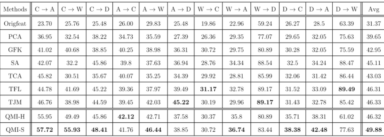
Each sub-problem is in the form of source→target, where C(Caltech-256), A(Amazon), W(Webcam) and D(DSLR) indicate four different domains. . . 41 2.2 Comparative results in terms of classification accuracy(%) of target

data for 12 different sub-problems. Each sub-problem is in the form of source→ target, where C(Caltech-256), A(Amazon), W(Webcam) and D(DSLR) indicate four different domains. . . 43 2.3 Classification accuracy(%) of target domain data for 12 different

sub-problems using SVM classifier (QMI-S [B]) andK-NN classifier (QMI-S [A]), both trained using projected source data. Each sub-problem is in the form of source → target, where C(Caltech-256), A(Amazon), W(Webcam) and D(DSLR) indicate four different domains. . . 45 2.4 Classification accuracy(%) of target data for 12 different sub-problems

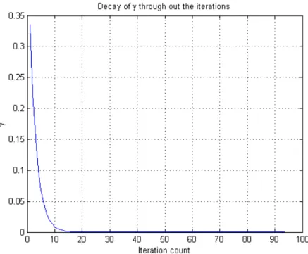
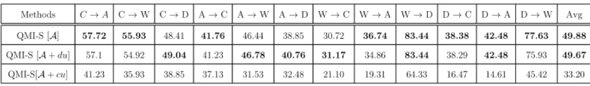
using K-nn classifier with K=1. Second row (QMI-S[A+du]) rep-resents accuracies where target predictions are obtained by adding a uniform uncertainty which is diminished through out the iterations (decayed uniform uncertainty). Third row (QMI-S[A+cu]) represents accuracies where target predictions are obtained with constant uniform uncertainty (γ = 0.5). . . 49

2.5 Average classification accuracy over all 12 sub-problems for different values of smoothing parameter (ρ) . . . 51 3.1 Comparative results in terms of classification accuracy(%) of target

do-main data for 7 different sub-problems using nearest neighbor classifier. Each sub-problem is in the form of source→target, where C(Caltech-256), A(Amazon), W(Webcam) and D(DSLR) indicate four different domains. . . 78 3.2 Classification accuracy (%) for target domain data using K-NN

clas-sifier trained with (I) all projected source points, (II) only projected source candidate points, (III) projectednon-candidate source points. 78 3.3 Comparative results in terms of classification accuracy(%) of target

data for 12 different sub-problems using the weighting scheme of source/target balancing. Each sub-problem is in the form of source→target, where C(Caltech-256), A(Amazon), W(Webcam) and D(DSLR) indicate four different domains. . . 84 4.1 Some possible partitions of a set 5 classes into two pseudo labels . . . 89 4.2 Classification accuracy (%) for target domain data in 7 different

sub-problems of Office+Caltech dataset. The last row represents the accu-racies achieved with the method described in this chapter. . . 94 4.3 att . . . 96 5.1 Classification accuracy(%) of target data for 12 different sub-problems

along with MI between data and corresponding labels using Newton-Lanzcos based nonlinear optimization . Each sub-problem is in the form ofsource→target, where C(Caltech-256), A(Amazon), W(Webcam) and D(DSLR) indicate four different domains. . . 103

LIST OF FIGURES

Figure Page

1.1 An example of transfer learning problem [1]. . . 2 1.2 Samples from different domains are represented by different features,

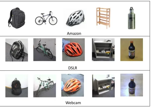
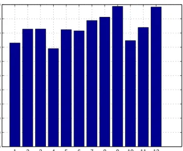
where red crosses, blue strips, orange triangles and green circles denote source positive samples, source negative samples, target positive sam-ples and target negative samsam-ples, respectively. By using two projection matrices P and Q, we transform the heterogenous samples from two domains into an augmented feature space. This picture is taken from [2]. 16 2.1 Proposed domain adaptation framework with two main steps. . . 35 2.2 Sample images from three different domains. . . 39 2.3 Number of target domain data (%) with reduced uncertainty of class

labels, upon convergence of iterative QMI-S. Each bar represents one sub-problem (source→target) indexed by {1, 2, . . . , 12}. . . 42 2.4 For each of 12 sub-problems, distance between 2 subspaces in

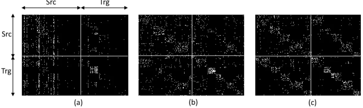
succe-sive iterations being decreased through out the iterations. Proposed algorithm reaches convergence when subspace distance is negligible. . 43 2.5 Assesing the quality of feature subspace by constructing similarity

ma-trix using projected source and target domain data (from 5 different classes) for sub-problem C → A using (a) original feature space, (b) TJM and (c) iterative QMI-S. . . 45

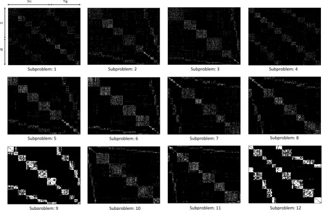
2.6 Similarity matrices S constructed with K nearest neighbors in learned subspaces for all 12 sub-problems. For each sub-problem, projected data (source and target) from 5 different classes are used to construct

S according to Equation (2.15). . . 46 2.7 Simulated annealing schedule for γ with the increase of iteration count. 48 3.1 Final subspace learned from Xs(blue shapes) and Xt(red shapes).

Circle, Rectangle and Star shapes represent three different object classes. Out-of-distribution source samples(light blue color) are distanlty lo-cated in the projected subspace. . . 59 3.2 Class label distribution (with four classes) for each source and target

domain datum. . . 60 3.3 Weighted K nearest neighbor approach to update a label prediction

of a target sample (marked as yellow). ‘S’and ‘T’represent source and target samples respectively. The updated label prediction will be p(c|x) = P4_i=1wip(c|xi), where wi is the corresponding weight of

each neighboring sample. . . 61 3.4 3-step iterative approach of the proposed framework based on

maxi-mization of WQMI-S. . . 62 3.5 Formation of candidate list Ω. . . 65 3.6 Proposed weighting scheme to be applied in iterative WQMI-S

algo-rithm for domain adaptation. . . 68 3.7 Plot of r vs. β. . . 70 3.8 3-step iterative approach of the proposed framework with intermediate

UPA approach at each iteration. In Step C, for each possible value ofτ

(say τ[i]), corresponding weight vector w[i] and M[i] are constructed to learn a subspace. . . 72

3.9 Comparison of source candidate size, source domain size and target domain size for each sub-problem. . . 79 3.10 Distribution of sourcecandidate points (%) among ten different classes

for each sub-problem. Each row represents one sub-problem and i-th column denotes percentile of source candidate from i-th class over all source candidate points. . . 80 3.11 Scatter plots of dm vs. weight of source domain data for 4 different

sub-problems. Source candidate points are higher weighted than non-candidate ones. The mean of dm distribution is idicated with red line

which is lower (higher) for source candidate (non-candidate) points. . 82 3.12 Illustration of distance vector constructed with dm values and

corre-sponding weight vector of 50 randomly selected source samples using colormap. Each sub-figure is representing one sub-problem. In each vector, a single stripe represents dm or weight of one sample. Higher

value of dm is associated with lower value of corresponding weight and

vice versa. . . 83 3.13 Illustration of projected data on WQMI-S subspace in 2d using t-sne

method [3]. The left column of sub-figures is for the sub-problem A→D and the right one for A→W. Each sub-figure is a two-dimensional vi-sualization of the learned subspace. (a and d) source and target point distributions in WQMI-S subspace , (b and e) same distributions with data annotated with class labels (represented as color) in WQMI-S sub-space, (c and f) class data distributions in TJM subspace. To assess the class discriminative nature of each subspace quantitatively, total scatter metric G is also reported. . . 85

4.1 Block diagram of the proposed method. Binary partiton of class labels is created and for each partition, a projection vector is learned inde-pendently by an iterative approach of WQMI-S maximization. Finally, all the projection vectors are stacked column wise to form a projection matrix. . . 94 4.2 Histogram plot of six randomly selected projection vector optimized

with binary class labels. Each sub-figure plots the 1-dimensional pro-jection of data along a propro-jection direction which shows a well-defined class separation of {C+, C−}. . . 95

CHAPTER 1

Introduction

In computer vision, object class detection or classification has been studied in both supervised and unsupervised settings. Traditional machine learning techniques try to learn a model based on a training data set and it is assumed that i) training and test data follow the same distribution, and ii) they are in the same feature space [4, 5]. These assumptions are often challenged in real life scenario. One major prerequisite of building most of these models is the availability of abundant labeled training images which might create a bottleneck, as it involves manual labor to annotate data. Also distribution of data changes over time. It is quite usual if the dataset on which a model is trained vary significantly from the data distribution during testing time [6–9]. This may cause poor model performance in terms of classification accuracy on the test set. Nevertheless, with the advance of image capturing and sensory devices e.g. DSLR (Digital Single-Lens Reflex) camera, webcam, mobile camera etc., enormous amount of image data are being generated at every moment. Therefore, the need for transfer learning may arise when the data can be easily outdated. In this case, the labeled data obtained in one time period may not follow the same distribution in a later time period. Hence, one of the challenges for building a model is to cope up with the emerging and ever-changing nature of dataset. Moreover, it is also assumed in traditional machine learning approach that the availability of labeled training examples in a dataset will be sufficient to build a model which will not face any novel category/instance or any variation or mutation of data during future testing. As for example, a model which is trained using indoor images captured

from canonical viewpoints of objects or categories, might perform poorly in outdoor settings. An example setting is provided in Figure 1.1. Therefore, a learning technique should be able to adapt to the changes across data distributions without requiring to train the model from scratch every time a new challenge appears. An adaptation method is required to reuse or transfer previously achieved knowledge for dealing with unknown samples or variation in test data distribution. In general, this research area is widely known as “Transfer Learning”.

Figure 1.1: An example of transfer learning problem [1].

In our research, we will investigate some issues of transfer learning problem and propose an efficient framework to deal with them. In this article, we will referdomain and dataset interchangeably. It is worth mentioning that this area is also known as domain adaption in literature [1, 10]. In a typical setting, there is a source domain where abundant labeled data are available or a trained model with available training samples are available for a specific task like classification, regression etc. There is another domain referred to as target where any combination of the following three cases may arise,

1. labeled data are in short supply. 2. the calibration effort is very expensive.

3. the learning process is time consuming and costly.

In this situation, sharing or transferring previous knowledge/experience from the source domain might be helpful to build a model in the target domain. The goal is to overcome the difficulties of the target domain to accomplish the task of interest. We already mentioned why these three situations may occur. This is a very interesting and challenging topic in current machine learning and vision based research which has direct impact on real life scenario. Therefore, I have decided to explore some of the issues in this area that can be dealt from different perspective or might need more attention for improvement. This type of topic is also exercised in Natural Language Processing (NLP), Sentiment classification and many other areas. It is assumed that although the data distributions in different domains is different, they share some com-mon characteristics in underlying low-dimensional manifold. The main challenge is to explore this underlying common structure or manifold across domains. Our research deals with the transfer learning problem and we propose an iterative framework to propagate knowledge from source to target domain in the form of class identity in-formation. The idea is to learn a common feature subspace such that data sharing underlying similarity (across domains) can be projected in close proximity on the learned subspace. This way, the divergence between source and target data can be minimized and then the labeled source data can be utilized to predict unlabeled tar-get domain data.

There are three main questions that need to be answered in the transfer learning area [1],

1. What to transfer? Before using previous experience or knowledge, we should be aware of what information we should utilize to learn a model that is suffer-ing from fewer trainsuffer-ing examples. This knowledge may come in various forms depending on the nature of the target task. Not all the information from an

available source domain might be effective in knowledge adaptation and this may affect the system performance. Identifying the source information as use-ful or non-useful might be a challenging task. In this research, we investigated this issue and provide a very simple but elegant approach to deal with this. 2. How to transfer? The next issue is how to efficiently apply the transferred

knowledge in order to facilitate model building in the target domain. This question is about the methodology that can connect the source knowledge to-wards target domain so as to efficiently explore the unknown or unlabeled target domain data.

3. When to transfer? This issue deals with the appropriate choice of the source knowledge that has been selected as a candidate for transfer. As for exam-ple, a model built on indoor home object images or office supply images is not a suitable candidate for learning a model that will identify school or campus decor objects, as these two domains do not share any features or characteris-tics among them. It is already mentioned that the domain difference might occur due to variability in capturing devices, images captured in different time domain, different resolutions, different surrounding environments and also dif-ferent canonical viewpoints. Whether the transferred knowledge is worthwhile in the target domain is another prime issue to address. In some cases, trans-ferring knowledge might cause performance bottleneck if we fail to apply it appropriately and when needed.

In our research, we propose a framework that will deal with these three issues inher-ently. The motivation was to utilize the underlying common shared structure to learn a low-dimensional subspace and propagate the source information towards unlabeled target data gradually. Our formulation is a ‘knowledge propagation’approach where ‘knowledge’refers to discriminative identity information of the available source model.

1.1 Terminology

In this section, some definitions and notifications are introduced that will be used through out this article. This section is highly influenced by the work of Pan and Yang [1].

Domain: A domain (D) or dataset is referred to as a collection of visual data. Each image is represented in a high-dimensional feature spaceX as a data point and a marginal distribution of data points is associated with a domain. In this research area, it is generally assumed that one domain follows a single marginal distribution. Thus a domain can be defined as D = {X, P(x)}. A domain might be referred to assource ortarget depending on the direction of knowledge transfer. Usually source domain is rich with label information i.e. each image is correctly annotated, whereas target domain suffers the availability of annotations and hence training a classification or regression model using only target domain data becomes impossible. Therefore, source domain data along with label information are utilized to explore the novel target domain in a transfer learning based approach.

Task: Given a specific domain, D={X, P(X)}, a task is referred to as learning a model f(.) (classification, regression etc.) to annotate unknown data in a label space Y. Therefore, a task T is defined as a tuple T = {Y, f(.)}. f(.) is generally an objective predictive function that is leaned using the domain data x ∈ X and corresponding label information y ∈ Y. For a single domain, data are sampled as training and testing set where training set contains data from different object cat-egories. The model is tested using the test data. Another approach is to partition the whole data set into three subsets: training, validation and testing set, where val-idation set is used to fine-tune the model parameter. This setting is used for various tasks, for example, object category detection, scene recognition, padestrian detection,

face recognition [11, 12] etc. It is worth noting that both training and testing data are sampled from the same marginal distribution, this setting might be challenged in real life scenario, e.g. if testing data come from a different distribution. Although the set of class labels is same across training and testing distributions, the marginal data distributions are different. This entails a bottleneck for a learned model to correctly identify the unknown test data.

In this research, we focus on this domain difference problem. It has been proven ex-perimentally that trained model performs poorly if the testing data are sampled from a different distribution. Therefore, it will be impractical to deploy a trained model without considering variability of unknown data. This necessitates model adaptation such that divergence difference is minimized. There are mainly two approaches for this adaptation:

1. Adapting a trained model by developing an adaptation layer on top of the model which will minimize the dataset bias. One popular approach is to utilize a Convolutional Neural Network model [13]. Usually a CNN is trained to learn a hierarchical features for images where intermediate layers represent mid-level image features. These mid-level features posses the characteristics of shared common structure. Therefore these features can be utilized to minimize the divergence gap between two different distributions.

2. Utilizing a label-rich large dataset for transferring knowledge i.e. if the labeled source and unlabeled target domain data are available, then they can be pro-jected in a common low-dimensional manifold subspace with a goal to utilizing their underlying common structure. On that projected space, the labeled source domain data can be used to predict the class identity of the unknown target domain data.

1.1.1 Definition: Transfer Learning

. Given a source domain Ds and learning task Ts, a target domain Dt and learning

task Tt, transfer learning aims to help improve the learning of the target predictive

function ft(.) in Dt using the knowledge of Ts inDs, whereDs 6=Dt or Ts 6=Tt [1].

According to the definition, as domain is defined as a pair D = {X, P(X)}, the condition Ds 6= Dt implies that either Xs 6= Xt or Ps(X) 6= Pt(X). For example, in

a task of document classification, there are both source document set and a target document set and either the term features are different between the two sets (e.g., they use different languages), or their marginal distributions are different. Similarly, a task is defined as a pair T = {Y, P(Y|X)}. Thus, the condition Ts 6= Tt implies

that eitherYs6=YtorP(Ys|Xs)6=P(Yt|Xt) [1]. When the target and source domains

are same, i.e. Ds =Dt and their learning tasks are same, i.e., Ts = Tt, the learning

problem becomes a traditional machine learning problem.

Given specific domains Ds and Dt, when the tasks Ts and Tt are different, then

either the label spaces between domains are different i.e. Ys 6=Yt or the conditional

probability distributions of theses domains are different i.e. P(Ys|Xs) 6= P(Yt|Xt).

In the document classification example, the former case corresponds to the situation where source domain has binary document classes whereas the target domain has 10 classes to classify the documents to. The latter case corresponds to the imbalanced situation in class distribution in source and target domains. In addition, the two domains are considered to be related if there exists some underlying shared structural similarity among the two domains.

1.2 Cases of Transfer Learning

Let source and target domains are represented by Ds and Dt respectively. In the

same way, source and target domain tasks are represented as Ts and Tt respectively,

their corresponding predictive functions are represented asfs(.) andft(.) respectively

and also their corresponding label spaces asYs and Yt respectively. According to the

definition of domain, the domain difference or distribution shift occurs (i.e Ds 6=Dt)

when either Xs6=Xt or P(xs)6=P(xt). Therefore, transfer learning deals with the

scenario where Ds 6= Dt and tries to learn a predictive function ft(.) by using the

knowledge inDs and the source predictive function fs(.).

Based on the definition of transfer learning, the following four cases are the possible scenarios where the transfer of previous knowledge is necessary,

Xs 6=Xt In this case, feature encodings across domains are different i.e. the feature

space where a model is trained is different from the feature space of the novel target domain. This difference might be the result of mismatch in dimensionality across domains or using different image representations. As for example, the same image or object can be represented as multiple feature representations, this line of research is also known as Heterogeneous Feature Adaptation (HFA) [14]. Usually a set of pivot features are detected across feature spaces to connect the two different feature distribution into a common shared feature set.

P(xs)6=P(xt) In this case, the marginal distributions of two different domains

(i.e. training and testing) are different. This scenario is commonly known as domain adaptation, distribution shift or dataset bias [10, 15, 15, 16]. Our research is focused on this issue with a goal to minimize the shift between this two marginal distributions. Here images from source and target domains are represented with the same feature encoding and also the label space are

same across domains. The goal is to identify the target domain data with a classification model that is mainly trained with the source domain data. This also minimizes the necessity of label information in target domain and adapts an already existing model to cope up with continuous evolving data set.

Ys 6=Yt This scenario is possible when the class data distribution is imbalanced.

In other words, if the source domain consists of p number of classes and the target domain consists of q number of classes, where p 6= q. Here the label space is different across domains. In the literature, this scenario is also known as zero-shot learning [17] or one-shot learning [18]. In zero-shot learning, no training data is available for the novel category in the target domain, whereas in one-shot learning, only one labeled training datum is available during training phase. Usually auxiliary information is harnessed to extract the underlying features existing in the novel category. This setting will be considered as a future extension of our current research so that the current proposed algorithm can handle the scenario of facing novel category that was not present during the training phase.

1.3 Settings of transfer learning

Based on the information available in source and target domain, several settings of transfer learning is possible, among them three common settings are: inductive transfer learning, transductive transfer learning and unsupervised transfer learning. Table 1.1 summarizes these three different scenarios. This table has been quoted from [1]. Here is a brief description of each of these settings.

Inductive transfer learning: In this setting, Ts 6= Tt i.e. the predictive target

functionft(.) is different from the one in the source domain. Therefore, source

infor-Table 1.1: Different settings of Transfer Learning. The table is adopted from [1]

.

Transfer Learning Setting

Related Areas Source Domain Labels

Target Domain Labels

Inductive TL Multi-task Learning Available Available

Self-taught Learning Unavailable Available

Transductive TL Domain Adaptation, Sample

Selection Bias, Co-variate Shift

Available Unavailable

Unsupervised TL Unavailable Unavailable

mation used in training a source model can be used as an auxiliary data for the target model. Although the target domain might not suffer from labeled data, researchers have been utilizing related auxiliary data from a different do-main to boost up the robustness or performance of the model. One example of this setting is to use semantic feature space for the corresponding object or image dataset and build a connection between image feature space and semantic feature space to enhance the quality of the trained model [19]. Based on the availability of the labled data in the source domain, this inductive setting can be further categorized into following two settings:

a. Labeled data in the source domain are available in plenty of amount. This scenario is often referred to as multi-task learning [20]. A significant dif-ference between multi-task learning and inductive transfer learning is that multi-task learning tries to optimize the function for both source and target task whereas inductive learning tries to learn a predictive function using target domain data along with utilizing the information available from the source domain data.

b. No labeled data are available in the source domain, this scenario is widely known as self-taught learning [21]. Rainaet al. first proposed a framework to utilize the knowledge of unlabeled source data that come from the same distribution as the labeled target domain data. Also the label

distribu-tion P(y) might be different across domains. This implies that unlabeled data might not be directly employed to learn a predictive model for the target domain, rather this information might act as a connecting auxiliary knowledge to help learn the target model.

Transductive transfer learning: In this setting, Ts = Tt but Ds 6= Dt i.e. the

tasks across domains are similar whereas the source and target domains are different either in terms of feature space or marginal probability distribution of data. Usually, target domain suffers from lack of labeled data causing difficulty to build a classification or regression model. This requires exploiting related source domain where plenty of labeled data are available. The term ‘transfer learning’is used for this setting in general. Based on the type of distribution of source and target domains, this setting is further categorized into following two sub-settings:

a. Here domain difference implies P(xs) 6= P(xt) although the images are

represented in the same feature space i.e. Xs=Xt. Also the two domains

have the same label space. This area is widely known as domain adapta-tion. In this research, we will mainly focus on this issue. Two different settings in domain adaptation (DA) are usually considered: i)unsupervised domain adaptation [7, 8, 22, 23], where no labeled data available in target domain; and ii) semi-supervised domain adaptation [24, 25], where only a few labeled data are available in target domain along with abundant labeled data of source domain. Some other related topics in the liter-ature that deal with domain adaptation include domain adaptation for knowledge transfer in text classification [26] , sample selection bias [27] or covariate shift [28].

data which was not present in the source domain during training phase. This implies that label space is different across domains i.e. Ys 6=Yt. The

goal is to identify the features that have similar characteristics distribu-tion among available source categories and the novel ones. Often a set of auxiliary information from web search is used in training to enhance the feature space for fitting novel category in the target domain [17, 29, 30]. Unsupervised transfer learning: This setting is similar to inductive transfer

learning except that this is an unsupervised learning method i.e. the task in target domain includes clustering, dimensionality reduction, density estimation etc [31,32]. In this case, no labeled data are needed in the target domain, hence source data are used in an unsupervised way to help train a model dedicated for the target task.

Our research will be focused on second setting oftransductive case whereP(Xs)6= P(Xt) and P(Ys|Xs) 6= P(Yt|Xt). The label space will be same across domains i.e. Ys=Yt. Nevertheless, in our research, we consider the tasks across domains be same

i.e. mainly focusing on classification or object recognition task across domains.

1.4 History of transfer learning

Broadly, three different types of approaches are found in the literature to deal with the above three cases of transfer learning settings. As our focus is on the trunsductive scenario, we performed our literature review based on that case only. Researchers have proposed a vast number of approaches to deal with the transfer learning issue, they can be roughly categorized as the following three approaches,

1. Instance based transfer.

3. Model parameter transfer.

The first context can be referred to as instance-based transfer learning (or instance transfer/ instance reweighting) approach [33–37], which assumes that a certain por-tion of the source domain can be potential candidate for knowledge transfer, hence source domain data are weighted based on their relevance with target domain data. In this scheme, the impact of non-relevant data are minimized by down-weighting them as they share the least common characteristics with target data. A second case can be referred to as feature-representation transfer learning approach [38, 39]. This can be also referred to as subspace learning based approach. The idea here is to learn a common ‘good’feature representation that can be used to encode both source and target domain image. Therefore the knowledge that will be transferred from source domain will be encoded in the feature encoding. This is intuitive as although the marginal distributions are different across domains, their underlying structure should be similar in a low-dimensional manifold. A third case can be referred to as parameter-transfer approach [13, 40] which reuse the parameter space learned using a label-rich source domain data. In this case the knowledge is transferred in the pa-rameter space. A fine-tuning step might be necessary to align the papa-rameter set to work for the target domain task, therefore available labeled data in the target domain is used to fine-tune this ’‘adaptation”layer.

1.4.1 Instance based transfer

This approach is based on correspondence relationship across domains using some pivot instances which are used to build a common shared model. Therefore, instance relationship should be known as prior information. In [19], a instance similarity has been applied along with some external semantic knowledge to propagate the source information for learning a target predictive function. Hoffman et al. propose a class invariant transformation function that projects the data points from one subspace to

another (source or target) with the help of instant constraints. This method uses both low-dimensional manifold structure and instance constraints to learn a feature space. A different approach is applied by Lim who tries to augment the source training data by for each class by borrowing example samples from other classes and learns a trans-formation function with the augmented set [41]. In [42, 43], authors propose to learn a similarity function using both source and target domain data and source label infor-mation both in linear and kernel form. This similarity function is plugged in various established classification models such that labeled source data are used for classifier training and unlabeled data are used for testing. Similar type of approach has been proposed by Donahue et al. [24] who tried to learn a smoothness regularizer to plug into an existing classification model. This smoothing function is learned with the help of instance relationship across domains. A geometric relationship among instances in the target domain is utilized by [44] which is known as low-rank reconstruction. The idea is that a point with same neighborhood class points in target domain can be reconstructed by the same neighboring class points in the source domain.

1.4.2 Feature representation based transfer/ subspace learning

In this category, a common image representation is sought in order to minimize the distribution divergence across domains and hence source data can be used to predict the identity of unknown target domain data. One of the case is, if data in differ-ent domains are encoded with differdiffer-ent image represdiffer-entations or they have differdiffer-ent dimensionality across domains. This scenario is known as Heterogeneous Domain Adaptation (HDA) [45]. Another approach is based on Heterogeneous Feature Aug-mentation (HFA) [2]. Here source and target domain data are represented with different feature spaces and hence two different projection matrices P and Q are learned for projecting them into a common feature space. This augmented feature space takes into account the original feature set and learned feature set with a goal to

build a large feature vector that will incorporate both common and individual char-acteristics among source and target domains (see Figure 1.2). A Feature Replication (FR) based approach has been applied in [39] i.e. each data x ∈ _Rd _{is augmented}

by extending its dimension upto three timesx∈_R3d_{. Therefore two different feature}

transformation function are learned to map the data as following, φs(x) = [x, x,0]T

and φs(x) = [x,0, x]T where φs(.) and φt(.) are learned for source and target domain

data respectively. This is also a feature augmentation based approach similar to [2] except that no projection or mapping was applied in this augmentation, only original raw feature space is used to augment the feature space. Although seems surprising, they provided promising results to support their framework.

Hoffman et al. proposes a domain-invariant feature representation with a goal to minimize the effect of distribution shift in the feature space [46]. As a part of the classification training process, they learn a feature mapping function that aligns the target domain features towards source domain. They propose a generic framework by optimizing feature space and classification jointly. Their method also supports large scale problem, heterogeneous domain adaptation and multi-class representation learning. Fei-feiet al. reused an old model built on unrelated categories to minimize the necessity of labeled images for the novel categories during training phase [47].The authors employed a Bayesian probabilistic framework to model the object categories along with prior information available in the source domain. Another line of work based on discriminative learning is widely used in NLP area [38]. A structural learning framework based on feature correspondence is proposed to establish a shared classifi-cation model across domains. Another issue of domain adaptation is the continuous evolving of data through out the time. Hoffman et al. deals with this issue where target data are considered to be samples from different subspaces and propose a novel framework for continuous manifold adaptation.

Figure 1.2: Samples from different domains are represented by different features, where red crosses, blue strips, orange triangles and green circles denote source positive samples, source negative samples, target positive samples and target negative samples, respectively. By using two projection matricesPandQ, we transform the heterogenous samples from two domains into an augmented feature space. This picture is taken from [2].

Recently subspace learning based methods have gain popularity because of their simplicity and effectiveness in learning process [7, 22, 48]. In these cases, authors utilize both source and target training data to learn a common low-dimensional sub-space with a goal to bring the two different distributions close together. Our work is somewhat related to this category, we propose a framework of subspace learning based on information theoretic perspective. Unlike others’ approach, we not only used the marginal distribution of source and target data, but also take the advantage of class conditional distribution of source domain data to build a discriminative common subspace.

1.4.3 Parameter transfer approach

In this approach, two major lines of work are widely practiced: one is to reuse the parameter set of an existing trained model as a initializer of the training process for the target domain task model, another is to employ the model parameters as a reg-ularization function in the objective function of target task model. Usually a model built using a large scale database is a suitable candidate for transfer learning using parameter transfer approach. Oquab et al. showed how a convolutional neural

net-work model trained with large image database can be efficiently applied to different tasks or different domains where labeled data is not sufficient to build a classification model. Mid-level image representations have been proved effective in transfer learn-ing scenario as they possess the common shared features across domains, therefore, the authors propose to train an adaptation layer by reusing the previously learned layer. This can alleviate the necessity of labeled target data even if the source task is completely different from the target domain task. Tommasi et al. proposed a model adaptation framework based on both parameter transfer and instance weighting ap-proach. Their work focuses on extending an SVM based model along with weighting previous knowledge in order to align the source domain with the target one. The work of Ayter et al. is also based on parameter transfer approach where they pro-pose to transfer the training of a detector model to identify a novel category in the target domain [40]. The previously learned object template has been adapted to act as a regularizer for the training of novel categories. Some other notable research in this category include hierarchical classification model to incorporate object hierar-chy structure [49], one shot learning utilizing class relevance metrics [50], adapting a Naive Bayes Nearest Neighbor classifier [51] etc.

1.5 Comparison methods

In next chapters, we propose our domain adaptation framework with exhaustive ex-perimental evaluations. We have used several benchmark datasets to prove the effi-cacy of the proposed model. We show that the proposed framework surpasses state-of-the-art approaches in most of the cases by a significant margin. We also conduct detailed experiments by varying parameter setting and analyzed the effect of them on the proposed method. Here we will provide a brief description of each of the method that are used for comparison, thanks to the authors of these methods to publish their codes online. Same experimental protocol has been followed to test the performance

by each method along with ours for a fair comparison. According to DA setting, labeled source data and unlabeled target data are applied to learn a common sub-space. Finally, the projected source data are utilized to annotate the unlabeled target domain data. In the following, the methods to be compared are described briefly.

1. Geodesic flow kernel [22]: This approach is based on finding a low-dimensional feature representation. The authors propose a kernel based method that model the underlying low-dimensional structure along the geodsic path from source to target domain. The model integrates an infinite number of subspaces which char-acterizes the domain shift in geometrical and structural properties along the path from source to target.

2. Subspace alignment [7]: In this method, source and target domain is rep-resented by their corresponding eigen spaces. An optimization function is designed to align the source domain with the target one. This mapping function projects cross-domain data into a low-dimensional subspace such that a classifier trained us-ing projected source data can be efficiently applied to projected unlabeled target data.

3. Transfer feature learning [23]: The authors propose a dimensionality reduction framework with a goal to minimize the distribution divergence between source and target domain data. Their method, known as Joint Distribution Adap-tation, jointly optimizes both the marginal and conditional distribution between domains. Their optimization criterion is the non-parametric Maximum Mean Dis-crepency (MMD) that measures the difference between the sample means of source and target data. The MMD criterion is integrated with PCA formulation to learn a low-dimensional subspace.

Transfer jont matching [8]: The authors propose a cross-domain feature rep-resentation which is invariant to both the distributions across domains and also the

irrelevant instances. They employ a feature matching and instance reweighting based technique to identify closely distributed source samples with target ones. The idea is to assign higher weights to source samples that are more relevant to the target domain data in order to minimize the impact of irrelevant data existing in the source domain.

Transfer component analysis [9]: Here the authors also use MMD metric to learn transfer components in a reproducing kernel Hilbert space. These transfer com-ponents will act as connecting landmarks between source and target domains such that in the projected subspace the difference in domain distributions is minimized. The authors prove that this new feature representation is suitable to use in traditional machine learning methods in order to classify unknown target domain data.

Principal component analysis [52]: This method is not intended for domain adaptation but has been used as a benchmark method for our proposed algorithm. PCA is an unsupervised dimensionality reduction technique with a goal to preserve maximum data variance in low-dimensions. We will project both source and target data into a PCA subspace and evaluate the classification accuracy achieved by a clas-sifier trained using projected source data. The performance evaluation will serve as a benchmark criterion for the need of domain adaptation or transfer learning.

CHAPTER 2

Subspace Learning Based On Quadratic Mutual Information Induced With Soft-labeling

In this chapter, a domain adaptation framework based on maximization of mutual information induced with soft-labeling has been proposed. In this problem setting, a source domain dataset with corresponding class labels and an unlabeled target do-main dataset are available. The goal is to learn a low-dimensional common feature subspace using both source and target domain data so that a classifier trained using projected source data can be applied to predict class labels for the unlabeled target domain data.

It is assumed that source and target data of a same class will be closely located in an ideal common subspace. A supervised technique based on maximization of non-parametric mutual information (MI) between data and corresponding class labels has been proved effective in learning such discriminative subspace [53–56]. Now to extend the prior work in domain adaptation setting, we induced soft assignment of class labels (probability that a point belongs to a class) into the objective function [53] of MI maximization. In the learned subspace, target data will be labeled softly using neighboring labeled source data. These two steps: i) finding MI-maximized subspace and ii) updating target data predictions will continue in an iterative fashion till converging to a final feature space. This iterative approach will aid to learn a domain-adaptive discriminative subspace utilizing both source and target domain data. In summary, our contributions in this work will be,

• utilizing class label distribution of source data along with all data across do-mains to develop a domain adaptation framework.

• extending supervised method of MI to support unlabeled target data by induc-ing soft-labelinduc-ing and

• proposing an iterative approach of common subspace learning based on maxi-mization of non-parametric MI with soft-labeling.

2.1 Mutual Information

According to information theoretic literature, Mutual Information (MI) is defined as a measures of independence between random variables [56, 57]. Assume a random variable X representing d-dimensional data points x∈ _Rd _{and another discrete}

ran-dom variableCrepresenting class labels fromc∈ {1,2, . . . , Nc}, whereNcis the total

number of classes. Also let p(x) is the marginal probability density function for the data samples, P(c) is the class prior probability and p(c) marginal distribution of class labels. Then MI is defined as,

I(X, C) =H(C)−H(C|X). (2.1) whereH(C) denotes the Shanon’s entropy or uncertainty of class labels [57] which is defined as,

H(C) =−X c

P(c) log(P(c)). (2.2) and H(C|X) is the class conditional entropy which is defined as,

H(C|X) = − Z x p(x) X c p(c|x) log(p(c|x)) ! dx (2.3)

Therefore,I(X, C) can be written as,

I

(

X, C

) =

−

P

P

(

c

) log

P

(

c

) +

R

p

(

x

) (

P

p

(

c|

x

) log

p

(

c|

x

))

Using the identities, p(c,x) = p(c|x)p(x) and P(c) = R_xp(c,x)dx, we can further simplify the above equation,

I(X, C) = −X c Z x p(c,x) logP(c) +X c Z x p(c,x) logp(c|x) =−X c Z x p(c,x) logP(c) +X c Z x p(c,x) log p(c,x) p(x) =X c Z x p(c,x) log p(c,x) P(c)p(x) =X c Z x p(x, c) log p(x, c) P(c)p(x) =KLp(x, c), P(c)p(x) (2.5) Whenp(x, c) = P(c)p(x), then the MI betweenCandXequals zero which essentially proves their independence of each other. MI can also be interpreted as the Kullback-Leibler divergence KL(,) between p(x, c) and the product of two distributions P(c) and p(x) [54].

2.1.1 Estimating MI: non-parametric approach

Estimating MI is a non-trivial task. Histogram-based approach is suitable for low-dimensional data and performs poorly in high-dimansional case [54]. The sparse nature of high-dimensional data makes it difficult for histogram based estimation. To overcome this, a non-parametric estimation based on parzen window has been pro-posed [54] following the formulation of Renyi’s non-parametric entropy [58]. Torkkola proposed a non-parametric quadratic measure of MI estimation, named as Quadratic Mutual Information (QMI). His proposed derivation of MI is inspired by Kapur [59]. Kapur argues that the third axiom of Shanon’s entropy can be relaxed in certain cir-cumstances. He tries to establish that instead of evaluating entropy of a distribution, we often focus on finding a distribution dm that minimizes/maximizes that entropy.

In this situation, the axioms for deriving the divergence measure (MI) can be relaxed and that optimization process can generate the desired distributiondm. This theory

leverages the options of a large number of entropy measure, one such outcome is Renyi’s entropy.

Following the above relaxation approach, Kapur also presented several non-parametric estimates of MI. Among those measures presented in [59], one is the following,

D

(

P

, P

) =

P

[

p

−

αp

q

+ (

α

−

1)

q

]

, α

6

= 0

, α

6

= 1

α = 2, ignore a constant and extend the discrete distributions to continuous ones as f1(x) and f2(x) respectively, the above equation of divergence measure becomes (following [54]),

D2(f1(x), f2(x)) = Z

x

(f1(x)−f2(x))2dx (2.7) It is possible to substitutef1(x) =p(x, c) andf2(x) =p(x), P(c) to derive a quadratic divergence measure between a joint distributionp(x, c) and a product of two distribu-tionsP(c) and p(x). Torkkola [54] also justified thatD2(,) eventually maximizes the lower bound ofKL(p(x, c), P(c)p(x)), that results in maximization of MI. Therefore, using Equation (2.7), QMI can be formulated as follows,

I(X, C) =X c Z x (p(x, c)−p(x)P(c))2dx =X c Z x p(x, c)2dx+X c Z x p(x)2P(c)2dx−2X c Z x p(x, c)p(x)P(c)dx (2.8) The probability distributions used in I(X, C) can be estimated by Parzen window method with a Gaussian kernel [60, 61]. A Gaussian function with mean µ and covariance matrix Σis defined as,

N (x;µ,Σ) = _p 1 2π|Σ| e −1 2(x−µ) T Σ−1 (x−µ)

We need to find expressions for P(c), p(x, c) and p(x) to compute MI according to equation (2.8). We will derive these expressions using Parzen window based density estimator [60]. Parzen-windowing estimates a probability density function (PDF)

p(x) from which samples were derived. Each observation is examined underneath a window function and size of the window determines the influence of that observation towards other samples inside that window. In this way, each samplexcontributes to the PDF estimate. While doing this, each sample is considered with equal importance. This assumption can be challenged in domain adaptation setting as we need to deal with two different distributions and our final feature space will be constructed with samples sharing similar underlying structures across two domains. Therefore, the approach will be not to assign equal importance (weight) for each sample. The closed form expression of MI presented in [53] is extended to a generalized version incorporating instance weighting and soft class assignment for target domain data. Hence, the main contribution to address domain adaptation problem using mutual information will be i) inducing soft class assignment into MI formulation for target domain data and ii) inducing instance weighting into QMI formulation to reduce the impact of unrelated samples (from both source and target domain) in learning a common subspace. Based on these attempts, we will derive closed-form expressions for,

a. Quadratic Mutual Information with Uniform Weighting of samples (UQMI) b. Quadratic Mutual Information with Non-uniform Weighting of samples (WQMI). In this chapter, the formulation of UQMI between data and corresponding class labels is presented. The goal is to learn a common subspace based on maximization of QMI between projected data and corresponding class labels. In next chapter, we will elaborately discuss about the WQMI approach. Each of this approach involves soft-labeling of samples i.e. instead of hard label annotation, each data point is associated

with a distribution of class labels.

2.1.2 QMI with uniform instance weighting (UQMI)

As stated earlier, we will now expand Equation (2.8) by substituting appropriate estimations of P(c),p(x, c) and p(x).

Evaluating P(x): A Parzen window density estimation of p(x) using IID drawn samplesxi is, p(x) = n X i=1 P(xi)N x;xi, σ2I

where n is the cardinality of data set. As the samples are un-weighted or uniformly weighted, P(xi) for each data sample can be expressed as P(xi) = 1_n and therefore p(x) becomes, p(x) = n X i=1 1 nN x;xi, σ 2_I

Evaluating P(c): P(c) is the prior class probability for class c ∈ {1,2, . . . , Nc}

which can be expressed as,

P(c) =

n

X

i=1

P(c| xi)P(xi)

NowP(c|xi) is the probability that xi belongs to a classc. Therefore, it indicates a

sample’s soft class labeling (probability of a datum being classified as class c). P(c) represents each sample’s class conditional probability, summed over all samples. We will denote this measure as Sc now on for notational convenience, that is,

P(c) = n X i=1 P(c|xi) 1 n =Sc

Evaluating p(x, c): A Parzen window estimate of the class data distributionp(x|c) is, p(x|c) = 1 P(c) n X i=1 P(c,xi)N x;xi, σ2I = 1 P(c) n X i=1 P(c|xi)P(xi)N x;xi, σ2I

= 1 Sc n X i P(c|xi) 1 n N x;xi, σ2I

Finally, the estimate ofp(x, c) i.e. joint pdf of xi and c takes the following form, p(x, c) = p(x|c)P(c) = 1 Sc n X i=1 P(c|xi) 1 n N x;xi, σ2I ! Sc = n X i=1 P(c|xi) 1 n N x;xi, σ2I = 1 n n X i=1 P(c|xi)N x;xi, σ2I

Using the expressions for p(x), P(c) and p(x, c) derived above, a closed form for Equation (2.8) will be formulated. As Gaussian kernel is used, we can define a centralized kernel matrix K∈_Rn×n _{asK =K˜ −E}

nK˜ −KE˜ n +EnKE˜ n , where

˜

Ki,j = N(xi −xj;0,2σ2I) and En is an n × n matrix with all elements equal

to 1/n. Let Φ∈ _Rn×m _{represents the mapped data points from raw feature space}

to a kernel Hilbert space using the mapping function ψ : X → H, where m is the dimension of kernel space (which is usually equals to infinity). Therefore,K =ΦΦT_. Following [53], Equation (2.8) can be represented as,

I(X, C) =Vin+Vall−2Vbtw (2.9) where Vin = X c Z x p(x, c)2dx = 1 n2 X c n X i=1 P(c|xi)N x;xi, σ2I !2 = 1 n2 X c n X i=1 n X j=1 P(c|xi)P(c|xj)N xi −xj; 0,2σ2I = 1 n2 X c n X i=1 n X j=1 P(c|xi)P(c|xj)Ki,j

= 1 n2 X c zcTKzc = 1 n2 X c trKzczcT = 1 n2tr ( ΦΦT X c zczcT ) = 1 n2tr ( ΦT X c zczTc ! Φ )

Herezc= [P(c|x1), P(c|x2), . . . , P(c|xn)]T ∈Rn×1. Vin essentially represents within

class potential [54] i.e. interactions between pairs of samples inside a class, summed over all classes. Therefore, maximizingI(X, C) will result in maximizing interactions between every pair of samples within a classcirrespective of their originating domains. Hence, this term will play a vital role in bridging data distributions of a specific class from two domains i.e. minimizing divergence in class conditional distributions (alternatively, divergence between Ps(c|xs) and Pt(c|xt) will be reduced between

source and target domains).

Vall = X c Z x p(x)2P(c)2dx =X c n X i=1 1 nN x;xi, σ 2_I !2 S_c2 =X c S_c2 n X i=1 n X j=1 1 n2N xi;xi, σ 2_I N xj;xi, σ2I =X c S_c2 n X i=1 n X j=1 1 n2N xi −xj;0,2σ 2_I = 1 n2 X c S_c2 ! _n X i=1 j=1 X j=1 Ki,j = 1 n2 X c S_c2 ! 1TK1 = 1 n2 X c S_c2 ! trK11T

= 1 n2 X c S_c2 ! tr ΦΦT11T = 1 n2 X c S_c2 ! trΦT11TΦ where 1= [1,1, . . . ,1]T ∈ _Rn×1_{. V}

all will control interactions between every pair

of samples weighted by squared sum of class prior probability, irrespective of their class labels and originating domains which will eventually ensure interactions between source and target domain data in our domain adaptaion setting.

Vbtw = X c Z x p(x, c)P(c)p(x)dx =X c 1 n n X i=1 P(c|xi)N x;xi, σ2I ! Sc n X j=1 1 nN x;xj, σ 2_I ! =X c Sc n X i=1 n X j=1 1 n2P(c|xi)N x;xi, σ 2_I N x;xj, σ2I =X c Sc n X i=1 n X j=1 1 n2P(c|xi)N xi −xj;0,2σ 2 I =X c Sc n X i=1 n X j=1 1 n2P(c|xi)Ki,j = 1 n2 X c SczcTK ·1 = 1 n2 X c trSc K·1·zcT = 1 n2tr ( X c Sc ΦΦT ·1·zTc ) = 1 n2tr ( ΦΦT ·1·X c SczcT ) = 1 n2tr ( ΦT 1·X c SczcT ! Φ )

Vbtw essentially represents interactions between class data points against all points.

In other words, it corresponds to interactions of a specific classcand all the available samples weighted by the prior of classc. According to Equation (2.9), minimizing this

term will eventually maximize MI between data points and corresponding class labels. Substituting the expressions for Vin, Vall and Vbtw into Equation (2.9), the closed

form expression of QMI will be,

I(X, C) = 1 n2tr ( ΦT X c zczcT ! Φ ) + 1 n2 X c Sc2 ! trnΦT11TΦo− 2 n2tr ( ΦT 1·X c SczcT ! Φ ) = tr ( ΦT ( 1 n2) X c zczcT ! + X c S2 c n2 ! 11T−2·1 X c Sc n2 ! zcT ! Φ ) = trnΦTMΦo. (2.10) where M = ( 1 n2) X c zczcT ! + X c S2 c n2 ! 11T −2·1 X c Sc n2 ! z_cT . (2.11)

M matrix is the core of the proposed subspace learning procedure. It essentially characterizes the subspace which is optimized based on maximization of mutual in-formation. The soft-labeling has been induced to original QMI formulation of [53] by the vectorzc= [P(c|x1), P(c|x2), . . . , P(c|xn)]T ∈Rn×1, we refer to this formulation

as QMI-S. Now maximizing QMI will eventually boils down to a trace optimization problem. In the next section, we will provide the objective function for learning a feature subspace cast as a trace ratio optimization approach.

2.1.3 Subspace Learning By Maximizing QMI-S

Now we can describe the objective function of the proposed algorithm for subspace learning based on the maximization of QMI between data and corresponding class la-bels, where instead of using hard labeling for each data point, a class label distribution (soft labeling) is used. Our formulation is inspired by the approach in [53]. Given a set of labeled data Xs ∈Rn×d from source domain (Ds) and unlabeled data Xt∈ Rn×d

from target domain (Dt), our input data matrix consists of X = [Xs,Xt] ∈ Rn×d, where n = ns+nt and ns and nt represent source and target data size respectively.

Computing QMI requires labeled data, whereas our target domain data is unlabeled. To overcome this issue, soft assignment of class labels for target data points are used. Each of these label distributions are initialized with uniform distribution of class la-bels (described in Section 2.1.6) and updated gradually in an iterative fashion.

As stated earlier, MI betweenX and C is measured in kernel space using mapped data pointsΦ. Therefore, data are first transformed into kernel space. Kernel matrix

K will be computed using kernel trick, K(xi,xj) =< φ(xi), φ(xj) >, where φ(x)

is a mapped datum from original feature space to a reproducing kernel Hilbert space using the mapping function ψ : X → H. We have mainly used Gaussian kernel in our thesis. By kernelizing the data matrix X, the goal is to find a k-dimensional feature subspace (k << m) using a linear transformation such that the QMI be-tween projected data and corresponding class labels (according to Equation (2.10)) is maximized. In other words, we need to find a projection matrix W ∈ _Rm×k _for

this transformation. W will transform the input data from kernel space to a low-dimensional feature space. Letwi is a projection vector fromW withwi ∈Rm. We

can impose a constraint onwi’s to be in the range ofΦi.e. they will span the kernel

feature space. Therefore, wi can be expressed as a linear combination of φ(x) i.e.

wi =

Pn

j=1ai,jφ(xj) = ΦTai, where ai ∈ Rn×1 is a coefficient vector. Projection

matrix W can be constructed by arranging each wi vector in columns such that

W = [w1,w2, . . . ,wn] = ΦTA, where A= {ai}ni=1 ∈ Rn

×k_{. Each column of A is}

ai, that is, Ai =ai. Using W, the projected data, XP ∈Rn×k can be obtained by

XP = ΦW. Our goal is to maximize QMI in the projected space. Therefore, the

QMI between data and corresponding class distributions in the learned space will be following,

Ip(Xp, C) = tr

(Xp)TM Xp

= tr

WTΦTMΦW

= trATΦΦTMΦΦTA

= trATKM KA (2.12)

Finding an optimal W now boils down to finding A with a goal to maximizing QMI. Hence the objective function for learning the QMI-maximized subspace can be represented as,

A∗ = arg max

AT_KA=Itr

ATKM KA (2.13)

The constraint in Equation (2.13) is derived from the orthogonality of the projection matrix W [53]. Here I represents identity matrix. This constraint can be deduced as, WTW =I ⇒(ΦTA)T(ΦTA) =I ⇒ ATΦΦTA=I ⇒ ATKKA =I. We will focus on casting the optimization problem in Equation (2.13) into a trace ratio optimization problem. In the next section, a brief overview on trace ratio optimization is provided.

2.1.4 QMI-S as a trace ratio problem

In the area of machine learning and pattern recognition, dimensionality reduction methods have been practiced and widely used. There exists a good number of su-pervised and unsusu-pervised dimensionality reduction techniques such as Linear Dis-criminant Analysis (LDA) [62], Principal Component Analysis (PCA) [52], Local Linear Embedding (LLE) [63], ISOMAP [64] and so on. Almost all of these meth-ods can be generalized as a trace ratio optimization problem which has been an active research topic in this area. This unified approach involves searching for a transformation matrix W that maximizes or minimizes a trace ratio of the form trWTSaW /tr

WTSbW where Sa and Sb are symmetric positive definite

Therefore, the trace ratio problem will take the following form, A∗ = arg max WT_W=I tr WT_S aW tr{WT_S aW}

This optimization problem suffers from an optimal closed form solution. Researchers have come up with an approximate solution by casting the above problem into an alternative ratio trace problem [65] defines as follows,

A∗ = arg max

WT_W=Itr

(WTSaW)−1(WTSaW)

The ratio trace problem can be solved by generalized eigen value decomposition (GEVD) method as Saul = βlSbul, where ul is the eigen vector corresponding

tol-th largest/smallest eigen value. The projection matrixW will be formed by the desired number of eigen vectors.

Researchers have argued that the above approximation approach is often far from optimal and tried to find a better solution. Besides GEVD approach, a number of other non-linear iterative techniques to the trace ratio problem has also been proposed in the literature [65–67]. In our work, the GEVD based solution is utilized because of its simplicity and fast implementation for the QMI-S optimization problem. Later in the thesis, we will incorporate a non-linear approach based on Newton’s method to solve the trace ratio problem in the proposed domain adaptation framework.

2.1.5 Solving QMI-S objective function

In order to cast the QMI-S optimization as a trace ratio optimization problem dis-cussed above, the following two constraints have been applied to Equation (2.13) according to [53],

i. Constraint 1: Often the class data happen to be imbalanced in either domains which makes the M matrix non-symmetric. To cast Equation (2.13) into a trace