IMPROVED PERMEABILITY PREDICTION USING
MULTIVARIATE ANALYSIS METHODS
A Thesis by JIANG XIE
Submitted to the Office of Graduate Studies of Texas A&M University
in partial fulfillment of the requirements for the degree of MASTER OF SCIENCE
December 2008
IMPROVED PERMEABILITY PREDICTION USING
MULTIVARIATE ANALYSIS METHODS
A Thesis by JIANG XIE
Submitted to the Office of Graduate Studies of Texas A&M University
in partial fulfillment of the requirements for the degree of MASTER OF SCIENCE
Approved by:
Chair of Committee, Akhil Datta-Gupta Committee Members, Yalchin Efendiev
Christine Ehlig-Economides Head of Department, Stephen A. Holditch
December 2008
ABSTRACT
Improved Permeability Prediction Using Multivariate Analysis Methods. (December 2008)
Jiang Xie, B.S., University of Science and Technology of China Chair of Advisory Committee: Dr. Akhil Datta-Gupta
Predicting rock permeability from well logs in uncored wells is an important task in reservoir characterization. Due to the high costs of coring and laboratory analysis, typically cores are acquired in only a few wells. Since most wells are logged, the common practice is to estimate permeability from logs using correlation equations developed from limited core data. Most commonly, permeability is estimated from various well logs using statistical regression.
For sandstones, often the logs of permeability can be correlated with porosity, but in carbonates the porosity permeability relationship tends to be much more complex and erratic. For this reason permeability prediction is a critical aspect of reservoir characterization in complex reservoirs such as carbonate reservoirs. In order to improve the permeability estimation in these reservoirs, several statistical regression techniques have already been tested in previous work to correlate permeability with different well logs. It has been shown that statistical regression for data correlation is quite promising in predicting complex reservoirs. But using all the possible well logs to predict permeability is not appropriate because the possibility of spurious correlation increases if you use more well logs. In statistics, variable selection is used to remove
unnecessary independent variables and give a better prediction. So we apply variable selection to the permeability prediction procedures in order to further improve permeability estimation.
We present three approaches to further improve reservoir permeability prediction based on well logs via data correlation and variable selection in this research. The first is a combination of stepwise algorithm with ACE technique. The second approach is the application of tree regression and cross-validation. The third is multivariate adaptive regression splines.
Three methods are tested and compared at two complex carbonate reservoirs in west Texas: Salt Creek Field Unit (SCFU) and North Robertson Unit (NRU). The result of SCFU shows that permeability prediction is improved by applying variable selection to non-parametric regression ACE while tree regression is unable to predict permeability because it can not preserve the continuity of permeability. In NRU, none of these three methods can predict permeability accurately. This is due to the high complexity of NRU reservoir and measurement accuracy. In this reservoir, high permeability is discrete from low permeability, which makes prediction even more difficult.
Permeability predictions based on well logs in complex carbonate reservoirs can be further improved by selecting appropriate well logs for data correlation. In comparing the relative predictive performance of the three regression methods, the stepwise with ACE method appears to outperform the other two methods.
DEDICATION
ACKNOWLEDGEMENTS
I would like to take this opportunity to express my deepest gratitude and appreciation to the people who have given me their assistance throughout my studies and during the preparation of this thesis. I would especially like to thank my advisor and committee chair, Dr. Akhil Datta-Gupta, for his continuous encouragement, financial support, and especially for his academic guidance. I would like to thank Dr. Christine Economides and Dr. Yalchin Efendiev for serving as committee members, and I do very much acknowledge their friendliness, guidance, and helpful comments while working towards my graduation.
I want to thank my friends in the reservoir characterization group, Dr. Xianlin Ma (now with Chevron), Dr. Deepak Devegowda (now in University of Oklahoma), Dr. Adedayo Oyerinde (now with ExxonMobil), Dr. Eduardo Jimenez (now with Shell), Sarwesh Kumar (now with Chevron), Prannay Parihar (now with Chevron), Jong-Uk Kim, Jichao Yin, Eric Bhark, Ajitabh Kumar, Ahmed Al-Huthali, Shingo Watanabe, Alvaro Rey and Qing Tao for making my graduate years very pleasant. I would also like to thank my Chinese friends Zhuoyi Li, Xiaoqing Wu, Jiaoyao Deng, Chang Liu and Ting He in the Harold Vance Department of Petroleum Engineering for their help.
I thank the various member companies of the Joint Industry Project for providing field data and funding. The facilities and resources provided by the Harold Vance Department of Petroleum Engineering, Texas A&M University, are gratefully acknowledged. I thank Texas A&M University for educating me in various ways, and by providing me with the very best education there is. I would like to take the opportunity to thank the faculty and staff helping me prepare for a life after graduation.
I am going to remember these years of hard work with great pleasure. To all of you, I appreciate what you have done to help me in my scholastic and professional growth. I would like to thank you for providing me with a work environment that lends itself to creativity and productivity, without too many financial concerns. Not everyone is so fortunate. I know I still have much to learn, but with continued support and encouragement from people like you I know I can accomplish a great deal.
NOMENCLATURE
ACE = alternating conditional expectations AIC = Akaike information criterion BIC = Bayes information criterion DPHI = density log derived porosity DT = acoustic transit time EF = electrofacies
GR = gamma ray log LLD = lateral log deep LLS = lateral log shallow
ΜΑΕ = mean absolute error
ΜΑRS = multivariate adaptive regression splines
ΜSE = mean squared error
MSFL = microspherically focused log NPHI = neutron log derived porosity NRU = North Robertson Unit RHOB = bulk density
RSS = residual sum of squares SCFU = Salt Creek Field Unit SP = spontaneous potential
α = cost complexity factor
TABLE OF CONTENTS
Page ABSTRACT ...iii DEDICATION... v ACKNOWLEDGEMENTS ... vi NOMENCLATURE ...viii TABLE OF CONTENTS ... ix LIST OF FIGURES... xiLIST OF TABLES... xiv
CHAPTER I INTRODUCTION ... 1 1.1 Literature Review... 1 1.1.1 Data Correlation ... 2 1.1.2 Data Partitioning ... 2 1.1.3 Variable Selection... 3 1.2 Objectives... 5
1.3 Two Field Cases: SCFU and NRU ... 6
1.3.1 Salt Creek Field Unit (SCFU) ... 6
1.3.2 North Robertson Unit (NRU)... 10
1.4 Error Measurement... 14
CHAPTER Page
II STEPWISE ALGORITHM ... 16
2.1 Introduction ... 16
2.2 Methodology ... 16
2.2.1 Response Transformation Models: ACE Algorithm... 16
2.2.2 Stepwise Algorithm ... 19
2.2.3 Combining ACE with Stepwise Procedure ... 20
2.3 Field Example: North Robertson Unit ... 21
2.4 Field Application: Salt Creek Field Unit... 29
2.5 Summary ... 41
III TREE REGRESSION ... 42
3.1 Introduction ... 42
3.2 Methodology ... 42
3.2.1 Regression Tree ... 42
3.2.2 Cross-validation and Pruning ... 43
3.3 Tree Regression Procedures ... 43
3.4 Field Application: Salt Creek Field Unit... 45
3.5 Field Application: North Robertson Unit ... 53
3.6 Summary ... 57
IV MULTIVARIATE ADAPTIVE REGRESSION SPLINES... 58
4.1 Introduction ... 58
4.2 Methodology ... 58
4.3 Procedure... 59
4.4 Field Application: Salt Creek Field Unit... 60
4.5 Field Application: North Robertson Unit ... 65
4.6 Summary ... 68
V DISCUSSION AND CONCLUSIONS ... 69
5.1 Discussion ... 69
5.2 Future Work... 71
REFERENCES... 72
LIST OF FIGURES
Page Figure 1.1 Location of Salt Creek Field Unit, Kent County, TX ... 7 Figure 1.2 Screenplot, A Barplot of the Variances of
the Principal Components ... 8 Figure 1.3 The Distribution of Electrofacies Data Plotted on
the First Two Principal Components of Well Logs ... 9 Figure 1.4 General Location of the North Robertson Unit ... 11 Figure 1.5 Location of Cored Wells in the North Robinson Unit ... 11 Figure 1.6 A Barplot Representing the Variances Described
by the PC’s ... 12 Figure 1.7 Electrofacies Characterization via Cluster Analysis... 14 Figure 2.1 Measured Permeability vs. Predicted,
W1509 NRU, Stepwise Regression... 27 Figure 2.2 Measured and Predicted Permeability vs. Depth,
W1509 NRU, Stepwise Regression... 28 Figure 2.3 Optimal Transform of GR in Electrofacies VII,
SCFU, ACE Algorithm... 31 Figure 2.4 Optimal Transform of LLD in Electrofacies VII,
SCFU, ACE Algorithm... 31 Figure 2.5 Optimal Transform of MSFL in Electrofacies VII,
SCFU, ACE Algorithm... 32 Figure 2.6 Optimal Transform of NPHI in Electrofacies VII,
Page Figure 2.7 Optimal Transform of PEF in Electrofacies VII,
SCFU, ACE Algorithm... 33
Figure 2.8 Optimal Transform of RHOB in Electrofacies VII, SCFU, ACE Algorithm... 33
Figure 2.9 Optimal Regression ln(Kg)_Tr vs. Sum_Tr_Indep of Electrofacies VII, SCFU, ACE Algorithm ... 34
Figure 2.10 Optimal Inverse Transform of Dependent Variable of Electrofacies VII, SCFU, ACE Algorithm ... 35
Figure 2.11 Cross plot of Fitted vs. Measured Permeability in Electrofacies VII... 36
Figure 2.12 Measured Permeability vs. Predicted Permeability, G517 SCFU, Stepwise ACE Algorithm ... 39
Figure 2.13 Measured and Predicted Permeability vs. Depth, G517 SCFU, Stepwise ACE Algorithm ... 40
Figure 3.1 Initial Regression Tree Model for Electrofacies I at SCFU... 45
Figure 3.2 Cross-validation of Electrofacies I at SCFU... 46
Figure 3.3 Optimal Regression Tree Model for Electrofacies I at SCFU ... 47
Figure 3.4 Measured Permeability vs. Predicted Permeability, G517 SCFU, Tree Regression ... 50
Figure 3.5 Measured and Predicted Permeability vs. Depth, G517 SCFU, Tree Regression ... 51
Figure 3.6 Measured Permeability vs. Predicted Permeability, W1509 NRU, Tree Regression... 55
Figure 3.7 Measured and Predicted Permeability vs. Depth, W1509 NRU, Tree Regression... 56
Page Figure 4.1 Measured Permeability vs. Predicted Permeability,
G517 SCFU, MARS... 63 Figure 4.2 Measured and Predicted Permeability vs. Depth,
G517 SCFU, MARS... 64 Figure 4.3 Measured Permeability vs. Predicted Permeability,
W1509 NRU, MARS ... 66 Figure 4.4 Measured and Predicted Permeability vs. Depth,
LIST OF TABLES
Page Table 2.1 Stepwise Regression Procedures and S-plus Report of
Electrofacies VII, NRU ... 21
Table 2.2 Regression and Prediction Errors of Full Linear model and Stepwise Linear Model of Electrofacies VII, NRU... 25
Table 2.3 Variables Selected of All Electrofacies, NRU ... 25
Table 2.4 Regression and Prediction Errors of All Electrofacies, NRU... 26
Table 2.5 Stepwise Procedure of Electroafacies VII, SCFU ... 30
Table 2.6 Regression and Prediction Errors of Electrofacies VII, SCFU ... 37
Table 2.7 Variables Selected of All Electrofacies, SCFU... 37
Table 2.8 Regression and Prediction Errors of All Electrofacies, SCFU ... 38
Table 3.1 Comparison of Regression and Prediction Errors of Initial Tree and Optimal Tree Model of Electrofacies I, SCFU ... 48
Table 3.2 Optimal Tree Size and Variables Selected for All Electrofacies, SCFU... 49
Table 3.3 Comparison of Regression and Prediction Errors of Initial and Optimal Tree Model for All Electrofacies, SCFU ... 49
Table 3.4 Comparison of Regression and Prediction Errors of Tree Regression and ACE for All Electrofacies, SCFU ... 52
Table 3.5 Comparison of Regression and Prediction Errors of Initial and Optimal Tree Model for All Electrofacies, NRU ... 53
Page Table 3.6 Comparison of Regression and Prediction Errors of
Tree Regression and ACE for All Electrofacies, NRU... 54
Table 4.1 Relative Variable Importance of Electrofacies I, SCFU... 60
Table 4.2 Basis Functions of Electrofacies I, SCFU ... 61
Table 4.3 Variable Selection of All Electrofacies, SCFU... 61
Table 4.4 Regression and Prediction Errors of All Electrofacies ... 62
Table 4.5 Comparison of MARS, ACE and Tree Regression ... 62
Table 4.6 Variables Selected of All Electrofacies, NRU ... 65
Table 4.7 Regression and Prediction Errors of All Eletrofacies, NRU ... 65
CHAPTER I
INTRODUCTION
1.1Literature Review
Predicting rock permeability from well logs in uncored wells is an important task in reservoir characterization. Due to the high costs of coring and laboratory analysis, permeability in most uncored wells is estimated using correlation equations developed from limited core data. Most commonly, permeability is estimated from various well logs using either an empirical relationship1, 2 or some form of statistical regression: parametric or non-parametric.1, 3-8 The empirical models may not be applicable in regions having different depositional environments without making adjustments to constants or exponents in the model. Also, significant uncertainty exists in the determination of irreducible water saturation and cementation factor in these models. Statistical regression has been proposed as a more versatile solution to the problem of permeability estimation. Conventional statistical regression is generally performed parametrically using multiple linear or nonlinear models that require a priori
assumptions regarding functional forms.3, 4
Three important aspects in predicting permeability using statistical regression are: 1. Data correlation
2. Data partitioning 3. Variable selection
1.1.1Data Correlation
In recent years, non-parametric regression techniques such as Generalized Additive Model (GAM)9, Alternating Conditional Expectation (ACE)4-6, 10-12 and Neural Networks (NNET)3 have been introduced to overcome the limitations of conventional multiple regression methods.1, 5-8 Applications to complex carbonate reservoirs have shown great promise in handling many forms of heterogeneity in rock properties. However, significant difficulties remain in the identification of sharp local variations in reservoir properties caused by abrupt changes in the depositional environment. Another distinctive feature in carbonate reservoirs is the porosity-permeability mismatch, that is, low permeability in regions exhibiting high porosity and vice-versa. These features are extremely important from the point of view of fluid flow predictions, particularly for early breakthrough response along high permeability streaks.
Lee’s work10 improves permeability predictions in heterogeneous carbonate reservoirs through a combination of electrofacies characterization and non-parametric regression techniques. Three non-parametric approaches are considered: ACE, GAM, and NNET. In this study, tree regression13, 14 and multivariate adaptive regression splines (MARS)15-17 are considered and compared to Lee’s results for a field case (Salt Creek Field Unit)
1.1.2Data Partitioning
Another important aspect in data correlation for permeability predictions is data partitioning. A variety of approaches have been proposed to partition well log responses into distinct classes in order to improve permeability predictions. The simplest approach utilizes flow zones or reservoir layering.6 Other approaches like lithofacies18, Hydrologic Flow Unit (HFU)7, 19-21 and electrofacies10, 11, 22 are explored and widely used. Previous work by Lee10 shows that electrofacies characterization with
the ACE algorithm, when compared against other data partitioning methods based on reservoir layering, lithofacies information and hydraulic flow units, gives a good permeability prediction. We will use electrofacies characterization as our data partitioning method and focus on other two aspects – data correlation and variable selection.
1.1.3Variable Selection
A spurious correlation is defined as a sample correlation that is large in absolute value purely by chance.23 Consider a well log as a possible predictor and the probability of observing the spurious correlation of this predictor is psc, we can calculate the probability of at least one spurious correlation when considering a set of k independent predictors, which is simply
(
)
∑
(
)
( ) = − − = − − k i i sc sc k sc p p p 1 1 1 1 1We can see that the penalty for increasing the number of predictors considered from k-1 to k is
(
)
( 1) 1− k− sc sc p pAs we use an increasing number of well logs, the chance of observing at least one spurious correlation increases. This is one of the reasons why we need to select appropriate variables for data correlation. Other possible problems with more well logs are:
1. Unnecessary predictor information will add noise to the estimation of other quantities that we are interested in.
2. Degrees of freedom will be wasted. Assume that n is sample size and k is number of independent variables, the degrees of freedom equalsd =n−k−1.
Degrees of freedom decreases as the number of independent variables increases.
Variable Selection is intended to select the “best” subset of predictors. Variable selection methods fall into two categories: best subset selection methods and stepwise regression methods. Best subset selection methods evaluate all the possible subsets of variables from a full model and identify the best reduced regression models based on some criterion. Evaluating all possible models is the most reasonable way to proceed in variable selection but it is computationally demanding, especially when one has a very large number of predictors. Stepwise algorithm is to evaluate the variables one at a time and look at a sequence of models.24
While stepwise algorithm is widely accepted for variable selection, pruning a regression tree may also be considered as a variable selection method. The difficulties of the stepwise algorithm and tree regression are the same: stopping criterion and optimal model selection. In the stepwise algorithm, a variety of criteria are available – AIC, BIC, adjusted R2, Predicted Residual Sum of Squares (PRESS) and Mallow’s Cp Statistic. We choose the AIC-criterion because the number of independent variables from AIC-criterion is a balance between model size and model regression error. In tree regression, cross-validation and AIC-criterion are two ways to select optimal tree size.13, 14 We choose cross-validation for tree regression because AIC-criterion tends to give a larger optimal tree size and over-fit in prediction.
1.2Objectives
The objective of this study is to further improve permeability prediction using well logs by variable selection and data correlation. First, stepwise regression is tested as a variable selection method. Then a method combining the stepwise algorithm and non-parametric regression is proposed and applied to a highly heterogeneous carbonate reservoir in the Permian Basin, west Texas: Salt Creek Field Unit (SCFU). Tree regression and multivariate adaptive regression splines (MARS) are performed for data correlation. Results are compared with non-parametric regression (ACE).
In statistics, stepwise regression is widely used for variable selection and model reduction. We start with stepwise regression as the linear regression model and apply it to North Robertson Unit (NRU) as a synthetic case in order to prove that stepwise algorithm can be used to improve permeability prediction. After that, a method combining the stepwise algorithm with non-parametric regression (ACE) is proposed and applied to Salt Creek Field Unit (SCFU). The result is compared with the ACE algorithm without variable selection.
In regression tree analysis, pruning might be considered as a method of variable selection14. Following this idea, we try to predict permeability using a regression tree and improve permeability estimation with a pruning tree. The key behind pruning trees is to select the optimal tree size. Cross-validation is a practical way to choose the optimal tree size. An AIC-criterion for pruning could also be used. Pruning with tree regression is applied to SCFU and NRU.
Another statistical regression method, multivariate adaptive regression splines (MARS), will be tested and applied to two field cases: SCFU and NRU. Results are compared with those from ACE algorithm.
1.3Two Field Cases: SCFU and NRU
In this study, we are focusing on data correlation and variable selection aspects of permeability estimations. We use electrofacies characterization for data partitioning.
1.3.1Salt Creek Field Unit (SCFU)
The Salt Creek field, located in Kent County, Texas, is a highly heterogeneous, shallow reef carbonate reservoir in the Basin shown in Figure 1.1. The reservoir lies on Strawn limestone and is overlain by the Cisco shale. The field consists of two major carbonate buildups: the South Main Body and the Northwest Extension. The buildup consists of grainstone shoals, bars and spits associated with a shelf environment. The average depth and thickness are 6300 ft and 170 ft respectively. The oil-water contact is located at -4425 ft subsea. Stratigraphically, the field can be subdivided into several vertical zones (labeled C5, C4, C3, C2b, C2a, C1b, and C1a) on the basis of paleontological picks and wireline correlations. Ten lithofacies have been identified from detailed core and thin-section studies: shale, siltstone, skeletal wackestone, algal wackestone, algal packstone, intraclastic packstone, skeletal/peloid packstone, peloid/skeletal mud lean packstone, peloid/sketetal grainstone, and ooid grainstone.4, 25
Figure 1.1 Location of Salt Creek Field Unit, Kent County, TX
In this study, we are focusing on the Northwest Extension area, which has 89 wells arranged in a 20-acre, five-spot pattern. The data presented in this analysis were collected from seven wells. We omitted two cored wells (G517 and G520) to verify our correlations with blind tests. 904 sample points from five wells are assigned as training data while 174 sample points from G517 and 183 sample points from G520 are assigned as prediction data. We have 10 well logs: caliper, spontaneous potential (SP), gamma ray (GR), three different resistivity (lateral log deep (LLD), lateral log shallow (LLS), and micro-spherically focused log(MSFL), acoustic transit-time (DT), neutron (NPHI), density (RHOB), and photoelectric logs (PEF). Seven well logs (GR, LLD, MSFL, DT, NPHI, RHOB and PEF) are selected out of ten well logs for data correlation and variable selection because of the similarity of the LLS and LLD responses, and also to account for the poor vertical resolution of SP and caliper logs.
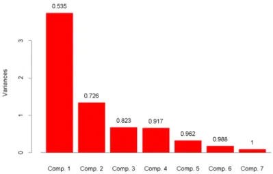
Figure 1.2 Screenplot, A Barplot of the Variances of the Principal Components labeled by ∑ = Σ j i i trace 1 ) ( / λ
Principal Component Analysis is applied to obtain the principal components PCj (j=1,…,7) from the well log data after normalization. Figure 1.2 shows the screen plot, a bar plot of the variance of the principal components labeled by
which often provides a convenient visual method of identifying the important components. Only 4 principal components explain around 90% variation of the whole data set. First principal component (PC1) appears to indicate porosity of the formation while second principal component (PC2) shows a stronger correlation with gamma ray readings. The eigenvectors of the covariance matrix provides coefficients of the principal components transformation. For example, PC1 and PC2 are given by
∑
= j i i trace 1 ) ( / Σ λ(
)
(
)
(
)
(
)
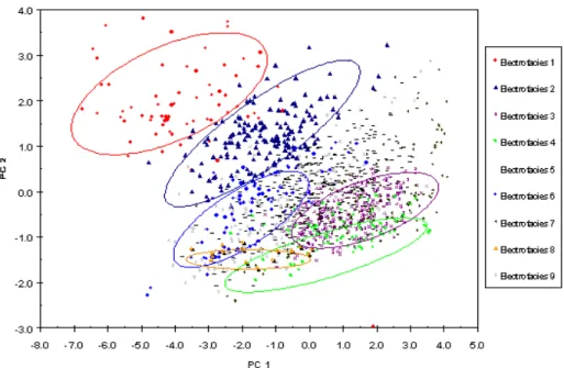
PEF . NPHI - . RHOB - . DT . MSFL . - LLD . -GR . PC PEF . NPHI . RHOB - . DT . MSFL . LLD . GR . PC 68 0 08 0 09 0 13 0 log 14 0 log 31 0 62 0 2 1 0 48 0 47 0 46 0 log 42 0 log 36 0 15 0 1 + = + + + + =Model-based Cluster Analysis is used to define 8 distinct groups based on the unique characteristics of the well log measurements. In Figure 1.3, each cluster can be treated as an electrofacies that reflects the hydrologic, lithologic, and diagenetic characteristics. Qualitatively speaking, the first electrofacies group (EF1) indicates tight media with low gamma ray reading and the eighth electrofacies group (EF8) represents porous media with high gamma ray reading.
-5 -4 -3 -2 -1 0 1 2 3 4 -6 -5 -4 -3 -2 -1 0 1 2 3 4 5 PC1 EF1 EF2 EF3 EF4 EF5 EF6 EF7 EF8
Figure 1.3 The Distribution of Electrofacies Data Plotted on the First Two Principal Components of Well Logs
1.3.2North Robertson Unit (NRU)
North Robertson Unit is a heterogeneous shallow shelf carbonate reservoir in Gaines County, west Texas. The NRU is located in the northern part of the Central Basin Platform of the Basin shown in Figure 1.4. There are two main producing horizons, the Glorieta and Clearfork Formations, often referred to as the Upper and Lower Clearfork, between the correlative depths of approximately 5874 – 7440 feet. The reservoir interval is thick (gross interval = 1400 ft). More than 90% of the interval has uniform lithology (dolostone), but is characterized by a complex pore structure that results in extensive vertical layering.7
Reservoir sediments accumulated in the Clearfork area of the Central Basin Platform were deposited in shallow, agitated waters providing a favorable environment for carbonate generation. Early winnowing in this high-energy environment provided primary intergranular porosity in some carbonates. However, fluctuations in relative sea level resulted in cyclic deposition typical of many Permian stratigraphic units in west Texas. Also, leaching and dissolution of skeletal grains, as well as selective dolomitization, modified porosity distribution significantly. In addition, local fractures and other late diagenetic processes affected the reservoir quality of the deposits, and the end result is a very heterogeneous and complex carbonate.7, 11
Figure 1.4 General Location of the North Robertson Unit
Figure 1.5 Location of Cored Wells in the North Robinson Unit
The data presented in this analysis were gathered from 6 cored wells and two wells (1509 and 3533) shown in Figure 1.5 are left out to verify our correlations using blind tests. 2630 sample points from six wells are assigned as training data while 712 sample points from W1509 and 851 sample points from W3533 are assigned as prediction data.
In this field, we have 9 well logs in different wells: caliper, spontaneous potential (SP), gamma ray (GR), two different resistivity logs (LLD and MSFL), acoustic transit-time or sonic (DT), neutron (NPHI), density (RHOB), and photoelectric (PEF). Only 6 well logs (GR, LLD, MSFL, DT, NPHI, and RHOB) are chosen because of their field-wide availability.
Electrofacies Characterization: Principal component analysis is used to summarize the data effectively and to reduce the dimensionality without any significant loss of information. This analysis is applied to obtain the principal components PCj (j=1,…,6) from the well log data after normalization.
Figure 1.6 A Barplot Representing the Variances Described by the PC’s
components labeled by
( )
∑
= ∑ l i i trace 1 / λ ,which often provides a convenient visual method of identifying the important principal components.
Only 3 principal components explain approximately 90% variation of the whole data set. First principal component (PC1) appears to indicate porosity of the formation while second principal component (PC2) shows a stronger correlation with gamma ray readings. The eigenvectors of the covariance matrix provides coefficients of the principal components transformation. For example, PC1 and PC2 are given by the following relationships
(
)
(
)
(
)
(
NPHI .)
RHOB - . DT . LLS . LLD . GR . PC NPHI . RHOB - . DT . LLS . LLD . GR . -PC 16 0 06 0 21 0 log 20 0 log 13 0 93 0 2 42 0 41 0 46 0 log 46 0 log 46 0 16 0 1 + + + = + + + =Next we apply model-based cluster analysis to define distinct groups based on the unique characteristics of the well log measurements. Each cluster can be treated as an electrofacies that reflects the hydrologic, lithologic, and diagenetic characteristics. The clustering algorithm indicates 9 distinct groups based on the well log measurements (Figure 1.7).
Figure 1.7 Electrofacies Characterization via Cluster Analysis
A qualitative interpretation of the clusters is aided by the relationship. For example, we can say that the first electrofacies group (EF1) represents porous media with high gamma ray reading and the ninth electrofacies group (EF9) represents tight media with low gamma ray reading.
1.4Error Measurement
In statistics, the mean squared error (MSE) and the mean absolute error (MAE) are two quantities used to measure the difference between prediction and true value. As the names suggest, the mean absolute error is an average of the absolute errors and the mean squared error is the second moment of the error:
(
)
(
)
(
)
(
)
∑
∑
= = − = − = − = − = N i i i i i N i i i i i y y N y y E MAE y y N y y E MSE 1 1 2 2 ˆ 1 ˆ ˆ 1 ˆ iy is defined as true value, yˆi as the prediction or estimator, and N is number of data. After permeability prediction with statistics regression, MSE and MAE are calculated to measure the prediction errors and compare different regression methods. Another measurement of data correlation for our approach is the correlation coefficient between measured permeability and predicted permeability.
( )
( )
y( )
y y y ˆ var var ˆ , cov = ρThe correlation coefficient indicates the degree of linear dependence between the variables. The closer the coefficient is to ±1, the stronger the correlation between the variables, which reflects our prediction accuracy.
1.5Thesis Outline
In Chapter II, we discuss stepwise algorithm as a variable selection method to improve non-parametric regression. Stepwise regression with a linear model is applied to illustrate the availability of the stepwise algorithm. A method combining the stepwise algorithm and ACE is proposed and applied to SCFU and NRU.
In Chapter III, we apply tree regression to permeability prediction and utilize cross-validation to select the optimal tree for variable selection. The results of SCFU and NRU from tree regression are compared with results from ACE.
In Chapter IV, the multivariate adaptive regression splines (MARS) method is compared with ACE. We utilize MARS software from Salford systems to perform multivariate adaptive regression splines.
CHAPTER II
STEPWISE ALGORITHM
2.1Introduction
In previous papers, electrofacies characterization and non-parametric regression ACE technique are proven to be successful in predicting permeability in highly heterogeneous carbonate reservoirs10, 11. In this chapter, we utilize the stepwise algorithm with AIC-criteria as a variable selection method to further improve permeability estimates. Stepwise regression is a kind of stepwise algorithm used in linear regression. We first demonstrate the availability of the stepwise algorithm by applying stepwise regression to North Robertson Unit (NRU). A method combining the stepwise algorithm and ACE is proposed and applied to field case Salt Creek Field Unit (SCFU). Results are compared with those from regression without variable selection.
2.2Methodology
In this section, we discuss the non-parametric regression technique, stepwise procedure and stepwise algorithm. A new method combining the stepwise procedure with ACE is proposed for permeability estimation.
2.2.1Response Transformation Models: ACE Algorithm14, 26
The response transformation models generalize the additive model by allowing for a transformation of the response variable y. The models have the following general form:
θ α ∑ φ ε = + + = p l l x l y 1 ) ( ) (
The main motivation behind response transformation is that often a simple additive model may not be appropriate for E(y | x1, x2,…,xp), but may be quite appropriate for
E{θ(y) | x1, x2,…, xp}. An example of such models is the Alternating Conditional
Expectation (ACE) algorithm.
The ACE algorithm, originally proposed by Breiman and Friedman26, is used here to derive the optimal transformations of the data to maximize the correlation between permeability and well logs. Let us say that we have a dependent random variable (for example, permeability) and independent random variables (for example, well logs). We first define arbitrary mean-zero transformations
Y p x x x1, 2...,
( ) ( )
y ,φ1 x1 ,...,φ2( )
xp θ .Suppose that a regression of the transformed dependent variable on the sum of transformed independent variables (under the constraint,E
[
θ2( )
y]
=1) results in the following error: 2 1 1 2( , ,..., ) {[ ( )∑
( )]} = − = p l l l p E y x e θ φ φ θ φ Then, transformations( ) ( )
y x *( )
xp 2 1 * 1 * ,φ ,...,φθ are said to be optimal for
regression if they satisfy the following
) ,..., , ( min ) ,..., , ( 2 1 ,..., , * * 1 * 2 * 1 p p e e p φ φ θ φ φ θ φ φ θ =
More details on the procedure to derive the optimal transforms can be found.6, 26 Briefly, our approach proceeds as follows:
Develop optimal non-parametric transforms for permeability and well log variables based on cored wells:θ
( ) ( )
y ,φ1 x1 ,...,φ2( )
xp ;corresponding transforms
{
( )
xli *( )
xpi}
1 *
1 ,...,φ
φ from step 1;
1. Estimate the optimal transform for permeability using the following relationship
( )
∑
( )
= = p l li l i x y 1 * * φ θ ;2. Finally, predict permeability through back transformation
( )
⎥ ⎦ ⎤ ⎢ ⎣ ⎡ =∑
= − p l li l pre i x y 1 * *1 φ θ .Thus, our calculation involves p forward transformations of
{
xli,...,xpi}
to
{
( )
xli *( )
xpi}
1 *
1 ,...,φ
φ , and a backward transformation. By restricting the transformation of the response variable to be monotone, we can ensure that is invertible. Non-parametric implies that no functional form is assumed between the dependent and independent variables and the transformations are derived solely based on the data set. The optimal correlation is given by plotting the transformed dependent variable against the sum of the transformed independent variables.
*
θ
Permeability is correlated with well logs within each electrofacies group using a non-parametric regression method. As mentioned before, the non-parametric regression allows us to correlate permeability with well logs without a priori assumptions regarding the functional form of the correlation. Specifically, a user-friendly software, GRACE (GRaphical ACE) is used for this purpose.
2.2.2Stepwise Algorithm24
Stepwise Procedures include backward elimination and forward selection. Backward Elimination is the simplest of all variable selection procedures and can be easily implemented without special software. The algorithm is as follows:
Start with all the variables in the model;
Remove the variable with highest p-value greater than critical; Refit the model and go to 2;
Stop when all p-values are less than critical.
The critical is sometimes called the “p-to-remove” and does not have to be 5%. If prediction performance is the goal, then a 15-20% cut-off may work best.
Forward selection just reverses the backward method: Start with no variables in the model;
For all predictors not in the model, check their p-value if they are added to the model. Choose the one with lowest p-value less than critical;
Continue until no new variable can be added.
Stepwise regression is a combination of the stepwise procedure and linear regression. In stepwise regression, Akaike Information Criterion (AIC) and Bayes Information Criterion (BIC) are two commonly used criteria. In general,
p
AIC =−2log−likelihood+2
while, BIC =−2log−likelihood+ plogn
p is number of variables and n is number of data.
For a linear regression model, the -2log-likelihood is known as the deviance, . In our study, we choose to minimize AIC in order to find the optimal model. Larger models will fit better and so have smaller RSS but use more parameters. Thus the best choice of model will balance fit with model size.
) /
log(RSS n
2.2.3Combining ACE with Stepwise Procedure
A new method combining the non-parametric regression technique (ACE) with the stepwise procedure is proposed. The general idea is to replace linear regression in stepwise regression with the ACE algorithm. We still utilize AIC criteria for model selection and use both backward elimination and forward addition in our stepwise procedure. The procedure is the following:
Fit the training data with the full model (all well logs) using ACE; Calculate AIC criteria;
Single term deletions and additions,
Non-parametric regression (ACE) with all new models, Calculate AIC criteria of new models;
If there is a smaller AIC value, select that model with least AIC value and repeat step2. If no model has smaller AIC than the initial model, stop the stepwise procedure and select initial model as the optimal model.
When we combine the stepwise algorithm with ACE technique, the basic procedure follows the stepwise procedure while the ACE technique is only used for model fitting. In stepwise regression, the basic procedure is the same but linear regression is used to fit the model.
2.3Field Example: North Robertson Unit
Stepwise regression is used for a field case to demonstrate how the stepwise procedure is performed. We will show that stepwise regression on North Robertson Unit improves the initial linear regression result.
Here, electrofacies VII is used as an example to show how stepwise regression works. Starting with the full model, which means that all six well logs (GR, DT, log10(LLD), log10(MSFL), NPHI and RHOB) are used, we follow stepwise procedure of backward elimination and forward addition. As each well log is added or eliminated, a linear regression is run and the AIC-criterion is calculated to compare with the optimal model from the last step until no more well logs can be added or eliminated. The following shows the stepwise procedure and stepwise regression result of electrofacies VII from an S-plus report.
Table 2.1 Stepwise Regression Procedures and S-plus Report of Electrofacies VII, NRU
Explanation S-plus Report
Starting full model with six well logs
*** Stepwise Regression ***
*** Stepwise Model Comparisons ***
Start: AIC= 273.0431
lnkcore ~ GR + NPHI + RHOB + DT + log.LLD. + log.MSFL.
Step 1
Backward elimination: (no forward addition because no well logs could be added)
Single term deletions
Model:
lnkcore ~ GR + NPHI + RHOB + DT + log.LLD. + log.MSFL.
Table 2.1 Continued
Explanation S-plus Report
Calculate regression models with only one well log eliminated.
Choose the best model with least AIC value.
Here, well log GR is eliminated. Df Sum of Sq RSS Cp <none> 230.5697 273.0431 GR 1 1.43069 232.0004 268.4061 NPHI 1 11.51604 242.0857 278.4915 RHOB 1 2.78198 233.3517 269.7574 DT 1 1.96724 232.5369 268.9427 log.LLD. 1 8.73986 239.3096 275.7153 log.MSFL. 1 6.83604 237.4057 273.8115 Step: AIC= 268.4061
lnkcore ~ NPHI + RHOB + DT + log.LLD. + log.MSFL.
Step 2
Backward elimination & forward addition:
Calculate regression models with only one well log eliminated or added.
Choose the best model. Here, well log RHOB is eliminated.
Single term deletions
Model:
lnkcore ~ NPHI + RHOB + DT + log.LLD. + log.MSFL. scale: 3.033812 Df Sum of Sq RSS Cp <none> 232.0004 268.4061 NPHI 1 10.09090 242.0913 272.4294 RHOB 1 2.62001 234.6204 264.9585 DT 1 2.90834 234.9087 265.2468 log.LLD. 1 7.31938 239.3198 269.6579 log.MSFL. 1 8.01270 240.0131 270.3512
Single term additions
Model:
lnkcore ~ NPHI + RHOB + DT + log.LLD. + log.MSFL. scale: 3.033812
Df Sum of Sq RSS Cp <none> 232.0004 268.4061 GR 1 1.430695 230.5697 273.0431
Step: AIC= 264.9585
Table 2.1 Continued
Explanation S-plus Report
Step 3
Backward elimination & forward addition
Well log DT is eliminated
Single term deletions
Model:
lnkcore ~ NPHI + DT + log.LLD. + log.MSFL. scale: 3.033812 Df Sum of Sq RSS Cp <none> 234.6204 264.9585 NPHI 1 10.41612 245.0365 269.3070 DT 1 1.03523 235.6556 259.9261 log.LLD. 1 9.57489 244.1953 268.4658 log.MSFL. 1 12.19701 246.8174 271.0879
Single term additions
Model:
lnkcore ~ NPHI + DT + log.LLD. + log.MSFL. scale: 3.033812 Df Sum of Sq RSS Cp <none> 234.6204 264.9585 GR 1 1.268725 233.3517 269.7574 RHOB 1 2.620006 232.0004 268.4061 Step: AIC= 259.9261
lnkcore ~ NPHI + log.LLD. + log.MSFL.
Step 4
Backward elimination & forward addition.
With single term deletion and addition, no other regression model is better than initial model in term of AIC criteria.
Single term deletions
Model:
lnkcore ~ NPHI + log.LLD. + log.MSFL. scale: 3.033812 Df Sum of Sq RSS Cp <none> 235.6556 259.9261 NPHI 1 15.3416 250.9972 269.2001 log.LLD. 1 46.7732 282.4288 300.6317 log.MSFL. 1 13.6257 249.2813 267.4842
Table 2.1 Continued
Explanation S-plus Report
Stepwise regression is stopped. Variables (NPHI, log10_LLD, log10_MSFL) are selected.
Model:
lnkcore ~ NPHI + log.LLD. + log.MSFL. scale: 3.033812 Df Sum of Sq RSS Cp <none> 235.6556 259.9261 GR 1 1.857994 233.7976 264.1357 RHOB 1 0.746895 234.9087 265.2468 DT 1 1.035225 234.6204 264.9585
Linear regression of optimal model is performed.
*** Linear Model ***
Call: lm(formula = lnkcore ~ NPHI + log.LLD. + log.MSFL., data = NRU.EF7, na.action
= na.exclude) Residuals:
Min 1Q Median 3Q Max -3.496 -1.119 -0.1982 0.6347 4.576
Coefficients:
Value Std. Error t value Pr(>|t|) (Intercept) -6.0195 1.0103 -5.9583 0.0000 NPHI 12.4082 5.4714 2.2678 0.0261 log.LLD. 1.6695 0.4216 3.9598 0.0002 log.MSFL. -0.7314 0.3422 -2.1372 0.0357
Residual standard error: 1.727 on 79 degrees of freedom Multiple R-Squared: 0.1834
F-statistic: 5.915 on 3 and 79 degrees of freedom, the p-value is 0.001078
After stepwise regression, an optimal model is selected, called the stepwise model. We perform regression and prediction with both the stepwise model and full model (all six well logs are used). Regression error and prediction errors of electrofacies VII are
shown in Table 2.2. From MSE and MAE of electrofacies VII, we can see that the stepwise procedure selects a generalized model and gives better predictions of well 1509 and 3533 compared to the full model. Thus, we can consider the stepwise algorithm as a variable selection and model reduction procedure.
Table 2.2 Regression and Prediction Errors of Full Linear model and Stepwise Linear Model of Electrofacies VII, NRU
Error Full model Stepwise model
MSE 2.7780 2.8392 Regression MAE 1.2667 1.3022 MSE 0.8885 0.6058 Prediction W1509 MAE 0.7355 0.6342 MSE 1.4308 1.0176 Prediction W3353 MAE 0.9763 0.8078
Table 2.3 Variables Selected of All Electrofacies, NRU Electrofacies Variables selected
I No variables
II RHOB, log10_LLD, log10_MSFL
III NPHI, RHOB, log10_LLD
IV NPHI, DT, log10_LLD
V GR, RHOB
VI NPHI
VII NPHI, log10_LLD, log10_MSFL
VIII NPHI, RHOB, DT, log10_MSFL
Table 2.3 shows the selected variables of each electrofacies. Different electrofacies represent different geologic zones or regions and can be characterized by specific variables. In electrofacies I, no variable is selected, which means that constant fitting is better than all other linear fits. This is the limitation of the linear regression model.
Table 2.4 Regression and Prediction Errors of All Electrofacies, NRU Error Full model Stepwise model
MSE 2.7724 2.8776 Regression MAE 1.2864 1.3225 MSE 1.3535 1.3376 Prediction W1509 MAE 0.8068 0.7661 MSE 2.8961 2.5827 Prediction W3353 MAE 1.0985 1.0712
The mean squared errors and mean absolute errors are compared in Table 2.4. Errors show us the improvement of the stepwise model in predicting permeability. The stepwise model gives larger regression error in training data because the stepwise model is a more general model for all data sets and the full model is more specific for this training data set. Table 2.4 shows that the stepwise procedure can be used as a variable selection method to improve permeability estimate.
10-3 10-2 10-1 100 101 102 103 10-3 10-2 10-1 100 101 102 103 Measured permeability P re d ic te d p e rm e a b ilit y MSE=1.3376 MAE=0.76611 ρ=0.195
Figure 2.1 Measured Permeability vs. Predicted, W1509 NRU, Stepwise Regression
From the comparison of measured permeability and predicted permeability in Figure 2.1 and Figure 2.2, we can not see a good permeability prediction. Figure 2.2 indicates that stepwise regression is unable to predict the general variation of W1509 and correlation coefficientρ =0.1950shows low linear dependency. This may be a result of the limitation of the stepwise regression method or the permeability data from
North Robertson Unit (NRU). 10-3 10-2 10-1 100 101 102 103 6000 6200 6400 6600 6800 7000 7200 7400 Permeability De p th
Measured permeability
Predicted permeability
Figure 2.2 Measured and Predicted Permeability vs. Depth, W1509 NRU, Stepwise Regression
2.4Field Application: Salt Creek Field Unit
The new method combining the stepwise algorithm with ACE technique is tested with data from Salt Creek Field Unit (SCFU). After electrofacies characterization, training data are grouped into eight electrofacies and data from G517 and G520 are used for a blind test and prediction.
We first apply the new method to electrofacies VII as a simple example: Table 2.5 summarizes the procedure of this method. In step1, the initial model is the full model with all seven well logs. After single term deletions and ACE regression, RSS (residual sum of squares), AIC and BIC criteria are calculated. The model with well log DT deleted is selected as the initial model for the next step.
In step2, we have the same single term deletions and additions and non-parametric regression. After calculation of the AIC citeron, we found that no other regression model is better than the initial model, thus the stepwise procedure is stopped and the optimal model is selected with six well logs (GR, log10_LLD, log10_MSFL, NPHI, PEF and RHOB). The optimal model will be applied to ACE. The following figures show the result of software GRACE.
Table 2.5 Stepwise Procedure of Electroafacies VII, SCFU
Step 1 RSS AIC BIC
7 logs 3961.819 308.6657 155.3264 - DT 3842.11 305.5331 152.2643 -DT - GR 4152.886 308.4043 155.1355 - log10(LLD) 5018.874 315.3962 162.1274 - log10(MSFL) 4276.268 309.4852 156.2164 - NPHI 4244.215 309.2075 155.9387 - PEF 4175.475 308.6047 155.3359 - RHOB 4335.877 309.9962 156.7274
Step 2 RSS AIC BIC
6 logs 3842.11 305.5331 152.2643 Stop - GR 4058.689 305.5575 152.3593 - log10(LLD) 5972.486 319.8179 166.6197 - log10(MSFL) 5274.891 315.2328 162.0346 - NPHI 4102.583 305.9546 152.7564 - PEF 4279.182 307.5103 154.3122 - RHOB 4238.882 307.161 153.9629
Optimal Transform
y = -1.5147E-03x3 + 3.8003E-02x2 - 2.0346E-01x - 2.5609E-01
R2 = 9.5336E-01 -2.50E+00 -2.00E+00 -1.50E+00 -1.00E+00 -5.00E-01 0.00E+00 5.00E-01
0.00E+00 5.00E+00 1.00E+01 1.50E+01 2.00E+01 2.50E+01
GR
GR_T
r
Figure 2.3 Optimal Transform of GR in Electrofacies VII, SCFU, ACE Algorithm
Optimal Transform
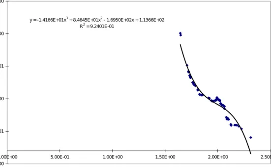
y = -1.4166E+01x3 + 8.4645E+01x2 - 1.6950E+02x + 1.1366E+02 R2 = 9.2401E-01 -1.00E+00 -5.00E-01 0.00E+00 5.00E-01 1.00E+00 1.50E+00
0.00E+00 5.00E-01 1.00E+00 1.50E+00 2.00E+00 2.50E+00
log10(LLD) lo g 10( LL D) _ T r
Optimal Transform
y = 2.5858E+01x3 - 1.3513E+02x2 + 2.3181E+02x - 1.3067E+02 R2 = 9.4128E-01 -1.00E+00 -8.00E-01 -6.00E-01 -4.00E-01 -2.00E-01 0.00E+00 2.00E-01 4.00E-01 6.00E-01
0.00E+00 5.00E-01 1.00E+00 1.50E+00 2.00E+00 2.50E+00
log10(MSFL) log1 0( M S FL) _ Tr
Figure 2.5 Optimal Transform of MSFL in Electrofacies VII, SCFU, ACE Algorithm
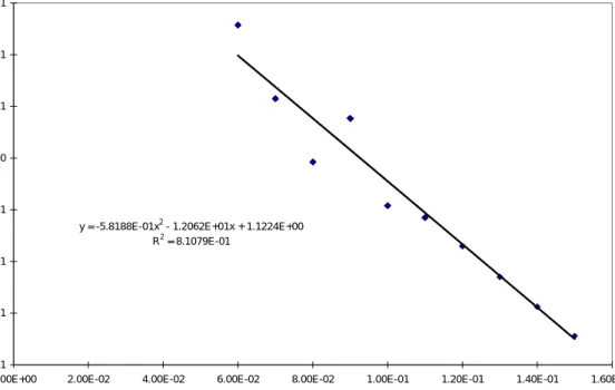
Optimal Transform
y = -5.8188E-01x2 - 1.2062E+01x + 1.1224E+00 R2 = 8.1079E-01 -8.00E-01 -6.00E-01 -4.00E-01 -2.00E-01 0.00E+00 2.00E-01 4.00E-01 6.00E-01
0.00E+00 2.00E-02 4.00E-02 6.00E-02 8.00E-02 1.00E-01 1.20E-01 1.40E-01 1.60E-01
NPHI
NPHI
_T
r
Optimal Transform
y = -6.0319E-01x2 + 6.9066E+00x - 1.9470E+01 R2 = 9.8938E-01 -8.00E-01 -6.00E-01 -4.00E-01 -2.00E-01 0.00E+00 2.00E-01 4.00E-01
0.00E+00 1.00E+00 2.00E+00 3.00E+00 4.00E+00 5.00E+00 6.00E+00
PEF
P
E
F_
Tr
Figure 2.7 Optimal Transform of PEF in Electrofacies VII, SCFU, ACE Algorithm
Optimal Transform
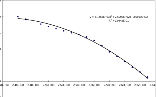
y = -5.1454E+01x2 + 2.5098E+02x - 3.0509E+02
R2 = 9.9342E-01 -1.50E+00 -1.00E+00 -5.00E-01 0.00E+00 5.00E-01 1.00E+00 1.50E+00
2.44E+00 2.46E+00 2.48E+00 2.50E+00 2.52E+00 2.54E+00 2.56E+00 2.58E+00 2.60E+00 2.62E+00 2.64E+00
RHOB
RHO
B_T
r
The general idea of non-parametric regression ACE algorithm is to transform independent and dependent variables into optimal space with maximized linear correlation. We utilized the GRACE software developed by Peter Valko and Akhil Datta-Gupta to perform the non-parametric regression ACE technique. Figure 2.8, Figure 2.4, Figure 2.5, Figure 2.6, Figure 2.7 and Figure 2.8 give the relations between independent variables and their transformed values. We fit those curves with polynomials in order to get simple correlations. In optimal space, we build a linear correlation between ln(Kg)_Tr and Sum_Tr (sum of all variables_Tr) in Figure 2.9. The correlation coefficient is 0.7089 for this case.
Optimal Regression, Correl:0.7089
-7.00E+00 -6.00E+00 -5.00E+00 -4.00E+00 -3.00E+00 -2.00E+00 -1.00E+00 0.00E+00 1.00E+00 2.00E+00 3.00E+00
-3.50E+00 -3.00E+00 -2.50E+00 -2.00E+00 -1.50E+00 -1.00E+00 -5.00E-01 0.00E+00 5.00E-01 1.00E+00 1.50E+00
Sum_Tr_Indep ln (K g )_ T r
Figure 2.9 Optimal Regression ln(Kg)_Tr vs. Sum_Tr_Indep of Electrofacies VII, SCFU, ACE Algorithm
Optimal Inv Transform
y = 2.2505E-01x2 + 1.7926E+00x + 3.4391E-01 R2 = 9.5822E-01 -4.00E+00 -3.00E+00 -2.00E+00 -1.00E+00 0.00E+00 1.00E+00 2.00E+00 3.00E+00 4.00E+00 5.00E+00
-7.00E+00 -6.00E+00 -5.00E+00 -4.00E+00 -3.00E+00 -2.00E+00 -1.00E+00 0.00E+00 1.00E+00 2.00E+00 3.00E+00
ln(Kg)_Tr
ln
(K
g
)
Figure 2.10 Optimal Inverse Transform of Dependent Variable of Electrofacies VII, SCFU, ACE Algorithm
Fitted Stdev = 1.1785 -4 -3 -2 -1 0 1 2 3 4 5
-4.00E+00 -3.00E+00 -2.00E+00 -1.00E+00 0.00E+00 1.00E+00 2.00E+00 3.00E+00 4.00E+00 5.00E+00
ln(Kg)_Meas Fr o m Fi t
GR_Tr= -1.5147E-03x3 + 3.8003E-02x2 - 2.0346E-01x - 2.5609E-01 log10(LLD)_Tr= -1.4166E+01x3 + 8.4645E+01x2 - 1.6950E+02x + 1.1366E+02 log10(MSFL)_Tr= 2.5858E+01x3 - 1.3513E+02x2 + 2.3181E+02x - 1.3067E+02 NPHI_Tr= -5.8188E-01x2 - 1.2062E+01x + 1.1224E+00
PEF_Tr= -6.0319E-01x2 + 6.9066E+00x - 1.9470E+01 RHOB_Tr= -5.1454E+01x2 + 2.5098E+02x - 3.0509E+02 ln(Kg)= 2.2505E-01 SumTr2 + 1.7926E+00 SumTr + 3.4391E-01
Figure 2.11 Cross plot of Fitted vs. Measured Permeability in Electrofacies VII
Figure 2.10 is an inverse transform of ln(Kg) from transformed space. Figure 2.11 is the final fitting vs. measured log-permeability. With polynomial equations from Figure 2.11, we are able to predict the new data set (G517 and G520) and calculate errors (MSE and MAE).
Table 2.6 shows the improved permeability estimate in terms of reduced errors. Compared to the full model, the optimal stepwise is a generalized model with better permeability prediction ability.
Table 2.6 Regression and Prediction Errors of Electrofacies VII, SCFU
Error Full model Stepwise model
MSE 1.2202 1.3895 Regression MAE 0.8697 0.9234 MSE 2.4793 1.0917 Prediction G517 MAE 1.1647 0.8439 MSE 1.7861 1.5227 Prediction G520 MAE 1.3361 0.7525
In order to apply the new method to all the other electrofacies, we select variables and obtain the optimal model for each electrofacies in Table 2.7 and then calculate the mean squared error and the mean absolute error in Table 2.8.
Table 2.7 Variables Selected of All Electrofacies, SCFU Electrofacies Variables Selected
I DT, GR, log10_MSFL, PEF
II GR, log10_LLD, log10_MSFL
III DT, GR, log10_LLD, PEF, RHOB
IV DT, GR, log10_LLD, log10_MSFL, RHOB
V DT, GR, log10_MSFL, NPHI, RHOB
VI DT, GR, log10_LLD
VII GR, log10_LLD, log10_MSFL, NPHI, PEF, RHOB VIII DT, GR, log10_LLD, log10_MSFL, NPHI, PEF, RHOB
Table 2.8 Regression and Prediction Errors of All Electrofacies, SCFU
Error Full model Stepwise model
MSE 1.58 1.6850 Regression MAE 0.97 1.1033 MSE 2.25 1.9728 Prediction G517 MAE 1.15 1.0682 MSE 1.74 1.8127 Prediction G520 MAE 1.04 1.0592
Finally, we plot measured permeability vs. predicted in Figure 2.12 and plot measured and predicted permeability vs. depth in Figure 2.13. Figure 2.12 indicates good linearity between measured permeability and predicted permeability with correlation coefficient = 0.6967. From Figure 2.13, we see that in general prediction is able to define the main feature of measured permeability vs. depth, but less successful in reproducing detailed extreme permeability. Permeability prediction is good considering that this is a highly heterogeneous carbonate reservoir.
10-3 10-2 10-1 100 101 102 103 10-3 10-2 10-1 100 101 102 103 Measured permeability P re d ic te d p e rm e a b ilit y MSE=1.9728 MAE=1.0682 ρ=0.68227
Figure 2.12 Measured Permeability vs. Predicted Permeability, G517 SCFU, Stepwise ACE Algorithm
10-3 10-2 10-1 100 101 102 103 6220 6240 6260 6280 6300 6320 6340 6360 6380 6400 6420 Permeability D ept h
Measured permeability
Predicted permeability
Figure 2.13 Measured and Predicted Permeability vs. Depth, G517 SCFU, Stepwise ACE Algorithm
2.5Summary
In this chapter, we discussed the stepwise algorithm, stepwise regression and proposed a new method combining the stepwise procedure with ACE algorithm to predict permeability. Our results show that the proposed method can improve permeability prediction under highly heterogeneous reservoir environments. Statistical software S-Plus is used for stepwise regression. Computer program GRACE (data correlation with ACE model developed by Peter Valko and Akhil Datta-Gupta) and manual stepwise procedure is performed with our new proposed method.
The following specific conclusions can be drawn based on this chapter:
1. The stepwise algorithm in conjunction with non-parametric regression (ACE) technique shows potential for permeability predictions in complex carbonate reservoirs.
2. An examination of the errors for uncored wells indicates that the stepwise algorithm potentially improves permeability estimation with both linear model and non-parametric regression model.
3. Variable selection and model reduction can be used further in permeability prediction.
4. Non-parametric regression techniques provide a practical tool for estimating permeability in heterogeneous carbonate reservoirs.
CHAPTER III
TREE REGRESSION
3.1Introduction
In this chapter, we discus regression tree and cross validation and their applications in data correlation and variable selection. The regression tree method is used to generate an initial tree model and cross-validation is used to find the optimal tree size. Cross validation and pruning tree together can be considered as a way of variable selection. After pruning, the optimal tree model is used to fit training data and predict the blind test data. Tree regression method is applied to both SCFU and NRU. Results are compared to non-parametric regression ACE.
3.2Methodology
3.2.1Regression Tree13, 14
A regression tree is built through a process known as binary recursive partitioning. This is an iterative process of splitting the data into partitions, and then splitting them further on each of the branches. Initially all of the records in a training set (the pre-classified records that are used to determine the structure of the tree) are lumped in one big box. The algorithm then tries breaking up the data, using every possible binary split on every field. The algorithm chooses the split that partitions the data into two parts such that the sum of the squared deviations from the mean in the separate parts is minimized. This splitting or partitioning is then applied to each of the new branches. The process continues until each node reaches a user-specified minimum node size and becomes a
terminal node. (If the sum of squared deviations from the mean in a node is zero, then that node is considered a terminal node even if it has not reached the minimum size.)
3.2.2Cross-validation and Pruning
Since the tree is grown from the training data set, when it has reached full structure it usually suffers from over-fitting (i.e. it is "explaining" random elements of the training data that are not likely to be features of the larger population of data). This results in poor performance on real life data. Therefore, it has to be pruned using the validation data set. Cross-validation13 is a very practical way to choose optimal tree size. It requires splitting data into k subsets, with a default choice of k=10. Each of the k subsets of the data is left out in turn, the model is fitted to the remaining data, and the results used to predict the outcome for the subset left out are compared with the initial tree regression results. In a regression model, prediction error is usually taken as the sum of differences between observed and predicted, that is, the criterion is the same as that used for the splitting rule.
Pruning can also be considered as a method of variable selection. AIC penalizes minus twice log-likelihood by twice the number of parameters. For regression tree, we can take . One way to select would be from the fit of the full tree model. But AIC-criterion tend to over-fit and choose larger constants14 because we usually underestimate from the full tree model.
2 ˆ 2σ α = σˆ2 2 ˆ σ
3.3Tree Regression Procedures
This section lists tree regression and cross-validation procedures and S-plus commands as an illustrative workflow. S-plus is an interface-based statistical software package; however, the command line can also be used to run the program. In the following
procedure, we find the optimal tree and make a prediction for each electrofacies. After predictions, mean squared error (MSE) and mean absolute error (MAE) are calculated. Procedure:
1. Generate full tree model with mincut = 2, minsize = 4, mindev = 10-6 and plot full tree,
tree.full <- tree(predictor ~ ., data = electrofacies, mindev = 10-6, mincut = 2, minsize = 4);
plot.tree(full.tree, “uniform”); text.tree(full.tree); 2. Cross-validation to find optimal tree size,
tree.cv <- cv.tree(tree.full, , prune.tree);
for (i in 2:5) tree.cv$dev <- tree.cv$dev + cv.tree(tree.full, , prune.tree)$dev; tree.cv$dev <- tree.cv$dev/5;
plot(tree.cv);
3. Prune full tree model to optimal tree size and plot optimal tree, tree.prune <- prune.tree(tree.full, best = optimal size);
4. Predict new data set with optimal tree model,
tree.predict <- predict.tree(tree.prune, newdata = list(), type=”vector”);
3.4Field Application: Salt Creek Field Unit
After electrofacies characterization, the training data set is divided into eight electrofacies. In each of electrofacies, tree regression is performed according to the workflow. Now we take electrofacies I as an example to demonstrate this regression tree method.
Figure 3.1 shows a regression tree for data correlation between the logarithm of permeability and well logs in electrofacies I. The numbers in each terminal node represent the final fitted logarithm of permeability for this regression tree model. This initial tree model has 47 terminal nodes and a residual mean deviance of 0.562. These attributes represent the complexity of the tree and its accuracy. The initial regression tree model is used to fit the training data itself and predict logarithm permeability in electrofacies I of the blind wells G517 and G520.
Using a cross-validation chart, we select the optimal tree size and prune the initial tree to this size. Figure 3.2 shows the cross-validation chart of electrofacies one and Figure 3.3 shows the optimal regression tree after pruning with an optimal tree size of 5. The number of terminal nodes is reduced from 47 to 5 with an increase in residual mean deviance of 0.562 to 1.799. However, the accuracy of the prediction should be improved by cross-validation and pruning.
1 10 20 30 40 size 36 0 380 4 00 42 0 440 4 60 dev ian c e 120.00 15.00 9.40 4.80 2.30 1.80 1.00 0.79 0.44 0.28 0.13
Figure 3.3 Optimal Regression Tree Model for Electrofacies I at SCFU
Next, we use the optimal regression tree model to fit training data and predict blind well G517 and G520. Table 3.1 is a comparison of regression error and prediction error of the initial tree model and optimal tree model for electrofacies I. The MSE and MAE result proves that a simpler tree structure leads to a better predictive ability because unseen samples are less sensitive to the statistical irregularities and idiosyncrasies of the training data.
Table 3.1 Comparison of Regression and Prediction Errors of Initial Tree and Optimal Tree Model of Electrofacies I, SCFU
Error Initial model Optimal model
MSE 0.3241 1.718
Regression error
MAE 0.4071 1.076
MSE Prediction error
G517 MAE No data in EF1
MSE 5.6609 4.2986
Prediction error
G520 MAE 1.8817 1.7656
The advantage of pruning and cross-validation is clear from Table 3.1. Moreover, pruning tree and cross-validation can be considered as a variable selection method to improve permeability prediction. In electrofacies I, only GR, RHOB and LLD are selected for data correlation out of seven well logs.
This above-stated workflow is repeated for the other seven electrofacies and the data from all electrofacies are combined. Table 3.2 shows the optimal tree size and, variables selected for all electrofacies and Table 3.3 shows regression error and prediction error of the initial and optimal models for all electrofacies. As expected, prediction errors of blind well G517 and G520 are all reduced and regression errors increase after pruning.
Table 3.2 Optimal Tree Size and Variables Selected for All Electrofacies, SCFU Electrofacies Optimal tree size Variables selected
I 5 GR, RHOB, LLD
II 6 RHOB, DT, PEF, MSFL, NPHI
III 3 RHOB
IV 4 GR, RHOB, LLD
V 2 LLD
VI 12 GR, RHOB, DT, PEF, MSFL, LLD, NPHI
VII 2 DT
VIII 3 GR, DT
Table 3.3 Comparison of Regression and Prediction Errors of Initial and Optimal Tree Model for All Electrofacies, SCFU
Error Initial model Optimal model
MSE 0.1995 1.4362 Regression error MAE 0.3031 0.9454 MSE 3.2761 2.2546 Prediction error G517 MAE 1.4278 1.1798 MSE 4.1523 3.0595 Prediction error G520 MAE 1.6867 1.4078
10-3 10-2 10-1 100 101 102 103 10-3 10-2 10-1 100 101 102 103 Measured permeability P re d ic te d p e rm e a b ilit y MSE=2.2546 MAE=1.1798 ρ=0.67573
Figure 3.4 Measured Permeability vs. Predicted Permeability, G517 SCFU, Tree Regression
10-3 10-2 10-1 100 101 102 103 6220 6240 6260 6280 6300 6320 6340 6360 6380 6400 6420 Permeability De p th Measured permeability Predicted permeability
Figure 3.5 Measured and Predicted Permeability vs. Depth, G517 SCFU, Tree Regression
Figure 3.4 shows a cross plot of predicted permeability vs. measured permeability of blind well G517. Figure 3.5 gives the plot of measured and predicted permeability vs. depth for well G517. From these two figures we observe that tree regression captures the general feature of measured permeability, but the limitation of tree regression is also obvious in that the same value tends to be assigned to different measured permeability because the average permeability prediction is given in each node and variation inside node is ignored. However, from the correlation coefficient