Citation for published version:
Petropoulos, F, Hyndman, RJ & Bergmeir, C 2018, 'Exploring the sources of uncertainty: why does bagging for time series forecasting work?', European Journal of Operational Research, vol. 268, no. 2, pp. 545-554. https://doi.org/10.1016/j.ejor.2018.01.045 DOI: 10.1016/j.ejor.2018.01.045 Publication date: 2018 Document Version
Peer reviewed version
Link to publication
Publisher Rights
CC BY-NC-ND
University of Bath
General rights
Copyright and moral rights for the publications made accessible in the public portal are retained by the authors and/or other copyright owners and it is a condition of accessing publications that users recognise and abide by the legal requirements associated with these rights. Take down policy
If you believe that this document breaches copyright please contact us providing details, and we will remove access to the work immediately and investigate your claim.
Exploring the sources of uncertainty:
why does bagging for time series forecasting work?
Fotios Petropoulosa,∗, Rob J. Hyndmanb, Christoph Bergmeirc
aSchool of Management, University of Bath, UK
bDepartment of Econometrics and Business Statistics, Monash University, Australia cFaculty of Information Technology, Monash University, Australia
Abstract
In a recent study, Bergmeir, Hyndman and Ben´ıtez (2016, Bagging exponential smooth-ing methods ussmooth-ing STL decomposition and Box-Cox transformation, International Journal of Forecasting 32, 303-312) successfully employed a bootstrap aggregation (bagging) tech-nique for improving the performance of exponential smoothing. Each series is Box-Cox transformed, and decomposed by Seasonal and Trend decomposition using Loess (STL); then bootstrapping is applied on the remainder series before the trend and seasonality are added back, and the transformation reversed to create bootstrapped versions of the series. Subsequently, they apply automatic exponential smoothing on the original series and the bootstrapped versions of the series, with the final forecast being the equal-weight combi-nation across all forecasts. In this study we attempt to address the question: why does bagging for time series forecasting work? We assume three sources of uncertainty (model uncertainty, data uncertainty, and parameter uncertainty) and we separately explore the benefits of bagging for time series forecasting for each one of them. Our analysis considers 4,004 time series (from the M- and M3-competitions) and two families of models. The results show that the benefits of bagging predominantly originate from the model uncertainty: the fact that different models might be selected as optimal for the bootstrapped series. As such, a suitable weighted combination of the most suitable models should be preferred to selecting a single model.
Keywords: forecasting, bootstrapping, aggregation, uncertainty, model combination
∗Correspondance: F Petropoulos, East Building, School of Management, University of Bath, Claverton Down, Bath, BA2 7AY, UK.
Email addresses: [email protected](Fotios Petropoulos),
[email protected](Rob J. Hyndman),[email protected](Christoph Bergmeir)
1. Introduction
Bootstrap aggregation (bagging) as proposed by Breiman (1996) is a technique that is well established in the machine learning community to reduce variance without increasing bias of the predictions and therewith to achieve more accurate point predictions (Hastie et al., 2009). In bagging, predictors are built on bootstrapped versions of the original data. The predictors form an ensemble, and predictions for new data are achieved by applying all predictors on the new data and then combining the results, by averaging for example. In this way, bagging includes different forms of uncertainty present when building a predictive model from data, namely data uncertainty, model uncertainty, and parameter uncertainty.
Though well established in machine learning contexts, it was not until recently that bagging has been applied successfully in a time series prediction context in the work of Bergmeir et al. (2016), yielding competitive results on the M3 competition dataset, especially on monthly data (Makridakis and Hibon, 2000). For time series, the main difficulty is that non-stationarity and autocorrelation have to be taken into account in the bootstrapping procedure, to produce bootstrapped samples that resemble the main characteristics of the original data. Also, in time series forecasting, relatively simple, low variance models have traditionally been used, rendering the expected gains of bagging as a variance reduction technique less promising.
In this paper, we perform a detailed analysis of how bagging addresses the different forms of uncertainties, to explore how and why bagging works. In particular, our aim is to isolate the different forms of uncertainty to analyse which of the uncertainties contribute most to model performance. In this way, we aim to find simpler, more directed ways of applying the bagging procedure in forecasting, and eventually produce even more accurate point forecasting methods.
The remainder of this paper is structured as follows. In Section 2, we present the current way bagging is used in time series forecasting. In Section 3, we propose a way to decompose and analyse the three sources of uncertainty in bagging. Section 4 shows the setup of the empirical experiments and the results. Section 5 discusses the managerial implications of the results and their importance to OR practice. Finally, Section 6 concludes the paper.
2. Bootstrapping and aggregation for time series
Two of the most popular univariate forecasting methods are exponential smoothing (Ex-ponenTial Smoothing or Error, Trend, Seasonality; ETS) and autoregressive integrated mov-ing average (ARIMA) models, both implemented in an automated fashion in the algorithms of Hyndman and Khandakar (2008). For a textbook introduction to these models, see Hyn-dman and Athanasopoulos (2014). We are interested in the application of bagging when forecasting from these well-known models.
The difficulty of bootstrapping in a time series context is that non-stationarity and autocorrelation have to be taken into account. A common way to approach this problem is to use a sieve bootstrap (B¨uhlmann, 1997), which fits a model and then bootstraps the residuals, assuming that they are uncorrelated. Following this approach, Cordeiro and Neves
(2009) fit ETS models to the data, and fit autoregressive (AR) processes to the residuals of the ETS models. Bootstrapped versions of a series can then be obtained by generating new residuals from the AR process, and combining them with the ETS model fit. However, their method has had limited success, and is often not able to outperform the base model. One reason for this may be that the method of Cordeiro and Neves (2009) does not allow the models for the bootstrapped series to be different from the model fitted to the original data. Consequently, model uncertainty is not addressed by their procedure.
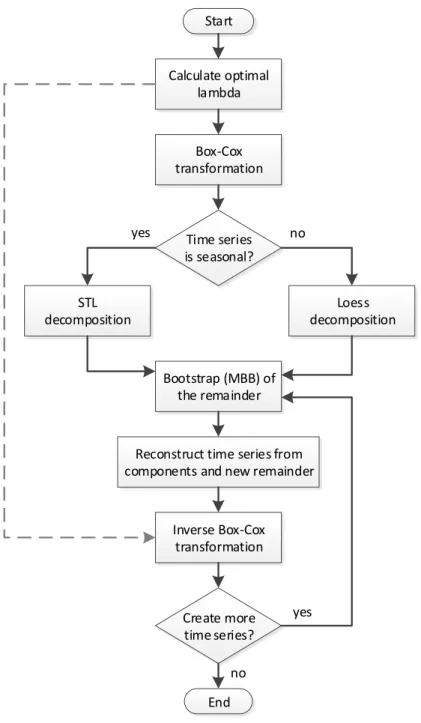
Our work builds on the bootstrapping procedure proposed by Bergmeir et al. (2016) (implemented in the function baggedETS in version 8.1 (and later) of the forecast package (Hyndman and Khandakar, 2008; Hyndman, 2017) in the programming language R (R Core Team, 2017)). This procedure tackles the difficulties of non-stationarity and autocorrelation in a different way from the approach of Cordeiro and Neves (2009). The procedure is outlined in Figure 1.
In a first step, a Box-Cox transformation (Box and Cox, 1964) is applied to the data, to stabilize the variance and to ensure that components of the time series are additive. The parameter λ of the transformation is chosen automatically using the procedure of Guerrero (1993).
Then, a decomposition procedure is applied to the series. If the data can exhibit season-ality (i.e., frequency >1, where “frequency” refers to the number of observations within a full season; i.e., 12 for monthly data, 4 for quarterly and 1 for yearly data), then Seasonal and Trend decomposition using Loess (STL, Cleveland et al., 1990) is applied to separate the series into trend, seasonal component and remainder. For non-seasonal time series (i.e., frequency = 1), a loess-based procedure (Cleveland et al., 1992) is employed to obtain a decomposition into trend and remainder, without a seasonal component.
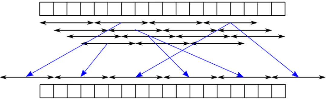
The remainder of the decomposition procedure can be assumed to be stationary, but it may be autocorrelated. Consequently, a bootstrapping procedure has to be used that takes autocorrelation into account. Bergmeir et al. (2016) considered the moving block boot-strap (MBB, K¨unsch, 1989). Figure 2 illustrates the procedure. However, other bootstrap algorithms could be used as well. For example, the circular block bootstrap (CBB, Politis and Romano, 1991) proposes that the time series is wrapped in a circle before resampling of blocks occurs. CBB is in theory superior to MBB as the`−1 first and`−1 last observa-tions of the series are not undersampled, where` is the blocksize. Another alternative is the more recently introduced linear process bootstrap (LPB, McMurry and Politis, 2010). While the block bootstrap algorithms produce data that mimic the original series, LPB has been “shown to be asymptotically valid for the sample mean and related statistics” (McMurry and Politis, 2010).
Once the remainder has been bootstrapped, the series is reconstructed from its structural components: trend, seasonality and the new, bootstrapped, remainder. By repeating this process, multiple new series, the bootstraps, are created. Then, a forecasting model is built for the original data and each of the bootstraps separately. In this work, we consider two families of models, namely ETS and ARIMA.
For ETS, an optimal model and set of parameters is identified for each series using the function ets() from the forecast package (Hyndman and Khandakar, 2008) for
the R statistical software (R Core Team, 2017)1. The input to the function is a vector of the original data values organised in a time series format. The output of ets() is a model form (together with the optimal parameters) consisting of three terms: error, trend and seasonality. The error term can be additive (A) or multiplicative (M). The trend and
1The analysis in this paper was performed with R 3.3.3 andforecastpackage 8.1.
Start End Box-Cox transformation Inverse Box-Cox transformation Calculate optimal lambda Time series is seasonal? STL decomposition Loess decomposition Bootstrap (MBB) of the remainder
Reconstruct time series from components and new remainder
Create more time series?
yes no
yes
no
Figure 2: Moving block bootstrapping of a time series. In a series with lengthnand blocksize`, n−`+ 1 possible blocks exist. In the example, the series has a length of 18 and blocksize is 4, so 15 blocks exist, as denoted by the arrows. The procedure then selects randomlybn/`c+ 2 blocks, and selects also randomly a starting point for the newly generated time series within the first block.
seasonal terms can be none (N), additive (A) or multiplicative (M). At the same time, if trend exists, this can be damped (d) or not. So, overall there exist 30 models. A model form is abbreviated as ETS(error, trend, seasonality). For example, ETS(M,Ad,N) refers to a model form with multiplicative error, additive damped trend and no seasonality. The function chooses the optimal model form according to an information criterion. In this work, we use the corrected Akaike information criterion (AICc) for model selection. By default, ets()excludes models with multiplicative trends from the search of an optimal model; we follow this option.
ARIMA models are fitted using theauto.arima()function from theforecast pack-age in a similar way. The function implements the Hyndman-Khandakar algorithm (Hynd-man and Athanasopoulos, 2014), which chooses an appropriate ARIMA model fully auto-matically. It uses repeated unit root tests to determine the number of differences to use, and the AICc to choose between models with different orders of the AR and moving average (MA) parts, up to a maximal order of 5 (which is the default parameter that we also use in our work).
In this way, a different model and/or set of parameters can be selected for each bootstrap, and a set of forecasts is produced from these models for each series/bootstrap. We note that, though the original work focused on ETS models only, we are considering ARIMA models as well, and potentially any other family of models can be used in this way.
The final point forecasts are calculated as an aggregation (combination) across all se-ries/bootstraps for each horizon. Following Bergmeir et al. (2016), we use the mean for aggregation, but also other functions, such as median, mode, or trimmed mean could be used.
3. Why does bagging work?
In this section we propose a decomposition of the benefits derived from bagging for time series based on three sources of uncertainty: data uncertainty, model uncertainty and parameter uncertainty. Subsequently, we present the forecasting strategies that will form the basis for our empirical evaluation (Section 4).
3.1. Data uncertainty
We apply the procedure described in the previous section to the time series with identi-fication N2136 from the M3-competition (Makridakis and Hibon, 2000). This is a monthly series covering a period of 10.5 years (126 observations). Figure 3 shows the original data values (in red) as well as 99 bootstraps (in blue) using a MBB for the remainder. It is evident that there exists variation in the resulting series. We call this variationdata uncer-tainty. This source of uncertainty could have an impact on model selection and parameter optimisation. 0 20 40 60 80 100 120 2000 4000 6000 8000 12000
Figure 3: Original series (red) and 99 bootstrap series (blue).
However, in an attempt to isolate the effect of data uncertainty, let us focus on a single model and a single set of parameters. We suggest that one reason that bagging for time series forecasting works is because the bootstraps will produce different forecasts from those produced by the original data. We expect that combining across these different sets of forecasts will render the final forecast resilient to the uncertainty observed in the data.
To check if this is the case, we fit to the original data an optimal exponential smoothing model, using the function ets() as outlined in Section 2. The optimal model form for the original data is the ETS(A,N,A), which refers to a non-trended model with additive seasonality. This model has two components, level and seasonality, with corresponding smoothing parameters, α and γ, as well as the initial states. As mentioned, apart from the model form, the function also returns the optimal values of these parameters. In this case, α = 0.3933 and γ = 0.0001. We now apply this model form and set of parameters to the bootstrapped series as well. Finally, the forecasts produced from the 100 time series (original and bootstraps) are combined with equal weights.
3.2. Model uncertainty
Next, we apply the ets() function to the bootstrapped series, allowing it to choose a different model each time. Given the variability of the random component, not all bootstraps
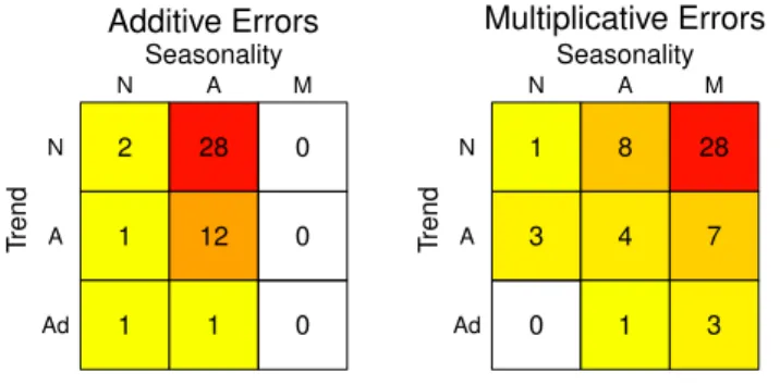
are expected to end up with the same optimal model. Indeed, Figure 4 presents the heat-map of the frequencies with which each model is identified as optimal for both the original data and the bootstraps. Note that the optimal model for the original data was the ETS(A,N,A). The same model form is identified as optimal in only 27 of the 99 bootstraps. Moreover, automatic model selection suggests the model with multiplicative seasonality and no trend in 28% of the series, while in 1/3 of the cases a model with additive trend (damped or not) is selected (i.e., the sum of the cases across both panels where a model has ‘A’ or ‘Ad’ trend equals to 33). Finally, note that as models with multiplicative trends have been excluded as a default option of ets(), their respective frequencies are zero and as such are not presented in Figure 4. Also, models with multiplicative seasonality must have multiplicative errors in order to avoid numerical instability; hence, these frequencies are also zero.
2 1 1 28 12 1 0 0 0 T rend N A Ad Seasonality N A M Additive Errors 1 3 0 8 4 1 28 7 3 T rend N A Ad Seasonality N A M Multiplicative Errors
Figure 4: Frequencies of optimal model forms for the original data and the 99 bootstraps. Left panel: additive error term. Right panel: multiplicative error term.
In balance, we observe variability in the identified optimal model form. We define this variability as model uncertainty. Following Box and Draper (1987), “all models are wrong” and selecting just one of these may not be enough. However, “some are useful” and efficiently combining those may lead to substantial improvements in forecasting performance. We suggest that another reason why bagging for time series forecasting works is because it can eliminate model uncertainty by selecting and applying a variety of models.
In order to isolate the effect of model uncertainty, we impose the unique identified optimal forms on the original data. In our example (Figure 4), 13 model forms are fitted to the data on top of the model form that has already been identified as optimal for these data (ETS(A,N,A)). Then weighted forecast combination can be applied, where the weights can be directly derived from the frequencies with which each model form has been identified as optimal. For example, the weight for ETS(A,A,A) will be 0.12.
3.3. Parameter uncertainty
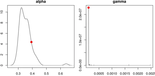
Even if the identified optimal model form for all bootstraps was the same as the original data, there would be differences with regards to the identified optimal values for the param-eters, which include smoothing parameters and initial states. For demonstration purposes, we focus here on the smoothing parameters only. As already mentioned, the optimal values when fitting ETS(A,N,A) to the original data were α = 0.3933 and γ = 0.0001. Figure 5
presents the density functions of the smoothing values identified as optimal for the boot-straps. We also present with red dots the optimal values of the original for comparison purposes. 0.3 0.4 0.5 0.6 0 2 4 6 8 10 alpha 0.0005 0.0010 0.0015 0.0020 0.0025 0.0e+00 1.0e+07 2.0e+07 gamma
Figure 5: Density function plots of the optimal smoothing parameters for the bootstraps. Smoothing parameters for the original data are presented with red dots.
We observe that for all bootstraps the optimalγ value is very low, and the most popular value coincides with the optimal smoothing γ value for the original data. However, this is not the case for the level smoothing parameter, α, where a range of values (0.24 to 0.68) is identified as optimal. Even more interestingly, the mode is 0.323, which is much smaller than the value identified as optimal on the original data. We define this variability in the identified optimal values as parameter uncertainty.
We propose, instead of using a single set of parameters (the one identified as optimal on the original data), to use all sets of parameters. The combination of these sets together with the single optimal model form should then be applied back to the original data. Thus, multiple sets of forecasts are produced using one model form, a single time series and multiple potentially optimal sets of parameters. Then, the forecasts should be combined using a suitable operator. Note that the bootstraps are not used here for producing forecasts directly, but only for identifying alternative sets of parameters.
3.4. Forecasting strategies
In this subsection we present the forecasting strategies that are implemented in this case study. These include standard model selection, model combination, bagging and three strategies that focus on isolating each one of the three sources of uncertainty.
Strategy 1 (simple benchmark)
Only the original series is used. A single model (and a single set of parameters) is selected automatically, based on information criteria. Subsequently, a single set of forecasts is produced. No combination or bootstrapping is used. This strategy links to the automatic
model selection approach for exponential smoothing or ARIMA models as described in Hyndman and Khandakar (2008).
Strategy 2 (model combination benchmark)
Only the original series is used. All possible models are fitted to the original data and parameters are optimised for each model separately. The forecasts produced from the different models are combined using weights derived from the values of information criteria (Kolassa, 2011). Note: this strategy is applied only on the exponential smoothing family of methods, as the ARIMA class is not finite.
Strategy 3 (bagging)
Both the original series and the corresponding bootstraps are used. Automatic model selection and parametrisation is performed on each series/bootstrap separately. A set of forecasts is produced from each series/bootstrap. The final forecasts are calculated as the trimmed mean (5%) across all series/bootstraps for each horizon. This is the bagging strat-egy described in Bergmeir et al. (2016).
Strategy 4 (bootstrap model combination)
Both the original series and the bootstraps are used. Automatic model selection is performed on each series/bootstrap separately. Each uniquely selected model form (for example: ETS(A,Ad,A)) is then applied back to the original data. Forecasts from the selected model forms are finally combined with weights corresponding to the frequency with which the respective models were identified as optimal. In other words, this is a weighted model combination approach, where the selected models and weights are directly derived from the application of automatic algorithms on the original data and the bootstraps. So, bootstraps are not used for producing forecasts directly.
Strategy 5 (bagging, single model & set of parameters)
Both the original series and the bootstraps are used. Automatic model selection and parametrisation are performed on the original data only. The identified optimal model form together with the optimal set of parameters is then applied to each one of the bootstraps for producing point forecasts. The final forecasts are calculated as the trimmed mean (5%) across all series/bootstraps for each horizon.
Strategy 6 (bootstrap parametrisation)
Both the original series and the bootstraps are used. Automatic model selection is performed on the original data only. The identified optimal form is subsequently applied on each one of the bootstraps, so that different sets of optimal parameters are generated. Then, the identified model form together with each one of the optimised set of parameters (as derived from the original series and the bootstraps) is applied back to the original series, thus producing several sets of forecasts. Finally, forecasts are calculated as the trimmed mean (5%) for each horizon. So, bootstraps are not used for producing forecasts directly, but only different sets of optimised parameters.
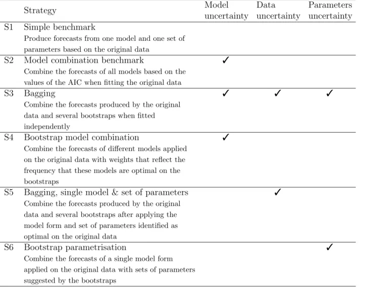
Table 1 summarises the various strategies considered and links them with the different sources of uncertainty dealt with in each case.
Table 1: Summary of the strategies considered along with the different sources of uncertainty dealt with in each strategy. Strategy Model uncertainty Data uncertainty Parameters uncertainty S1 Simple benchmark
Produce forecasts from one model and one set of parameters based on the original data
S2 Model combination benchmark 3
Combine the forecasts of all models based on the values of the AIC when fitting the original data
S3 Bagging 3 3 3
Combine the forecasts produced by the original data and several bootstraps when fitted independently
S4 Bootstrap model combination 3
Combine the forecasts of different models applied on the original data with weights that reflect the frequency that these models are optimal on the bootstraps
S5 Bagging, single model & set of parameters 3
Combine the forecasts produced by the original data and several bootstraps after applying the model form and set of parameters identified as optimal on the original data
S6 Bootstrap parametrisation 3
Combine the forecasts of a single model form applied on the original data with sets of parameters suggested by the bootstraps
4. Empirical investigation 4.1. Design
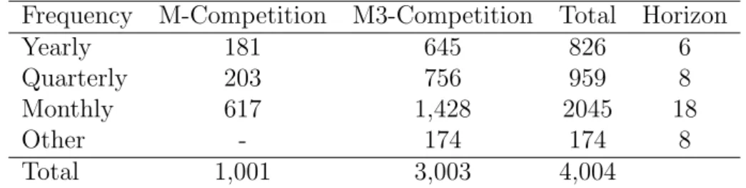
To empirically compare the six strategies presented in Section 3.4, we use the time series from the two most cited competitions to-date, the M (Makridakis et al., 1982) and M3 (Makridakis and Hibon, 2000) forecasting competitions. Together, these comprise 4,004 series of various frequencies and lengths. Table 2 presents in more detail the number of time series per data set and frequency, along with the forecasting horizon for each frequency as required in the original competitions. We opt to keep the same lengths for the in-sample test sets to allow comparability with published results.
Table 2: Time series per data set and frequency.
Frequency M-Competition M3-Competition Total Horizon
Yearly 181 645 826 6
Quarterly 203 756 959 8
Monthly 617 1,428 2045 18
Other - 174 174 8
Total 1,001 3,003 4,004
For each time series, we generate 99 bootstraps following the procedure presented in Figure 1. Instead of applying a formal test on the original data to check if the time series is seasonal or not, STL decomposition is applied to all series with periodicity higher than unity. Our argument is that even if seasonality is weak, the re-sampling of the remainder could result in better capturing and modelling of seasonal patterns. In other words, even if a seasonal model is not optimal for the original data, a seasonal model may still be used for some of the bootstraps. If Loess decomposition is applied instead of STL, then the bootstrapping procedure would essentially remove any seasonal patterns and seasonality would not be identified at any of the bootstraps.
The bootstrapping of the remainder is produced using three algorithms: MBB, CBB and LPB. The following Section (4.2) presents results produced using the MBB algorithm. Results based on CBB and LPB are discussed in Section 4.4 and are presented in the Appendix.
The forecasting performance of each approach is measured via the symmetric Mean Absolute Percentage Error (sMAPE) and the Mean Absolute Scaled Error (MASE). The former, despite its disadvantages, allows for comparisons with previously published results on the same data. The latter is a popular error measure that has been proposed more recently (Hyndman and Koehler, 2006). MASE is a scaled variant of the Mean Absolute Error (MAE), where the scaling is equal to the MAE of the seasonal random walk for the in-sample data. sMAPE and MASE for a single time series are defined as follows:
sMAPE = 200 H H X h=1 |yn+h−fn+h| |yn+h|+|fn+h| , (1) MASE = (n−m) H X h=1 |yn+h−fn+h| H n X t=m+1 |yt−yt−m| , (2)
where yt is the observation at time t, ft is the forecast at period t, n is the length of the
in-sample,H is the forecasting horizon, andm is the number of periods within a season (12 for monthly data).
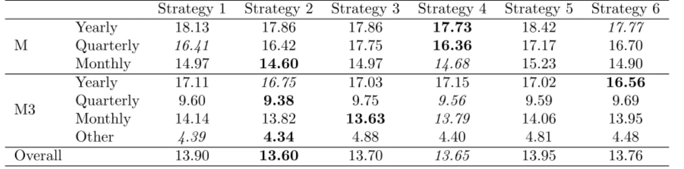
Table 3: Average sMAPE (%) of the different forecasting strategies for ETS models and different data sets. Strategy 1 Strategy 2 Strategy 3 Strategy 4 Strategy 5 Strategy 6 M Yearly 18.13 17.86 17.86 17.73 18.42 17.77 Quarterly 16.41 16.42 17.75 16.36 17.17 16.70 Monthly 14.97 14.60 14.97 14.68 15.23 14.90 M3 Yearly 17.11 16.75 17.03 17.15 17.02 16.56 Quarterly 9.60 9.38 9.75 9.56 9.59 9.69 Monthly 14.14 13.82 13.63 13.79 14.06 13.95 Other 4.39 4.34 4.88 4.40 4.81 4.48 Overall 13.90 13.60 13.70 13.65 13.95 13.76
4.2. Results based on the MBB
In this section we provide results based on the MBB. Tables 3 to 4 present the results for sMAPE and MASE respectively, where ETS is used as the forecasting model. The different data sets are presented in rows and the different strategies proposed in Section 3.4 are presented in columns. Also the last row offers the arithmetic mean across all data sets, weighted based on the size of each data set (see Table 2). For each row (subset of data), the best and second-best strategies are presented in boldface and italics respectively.
Table 3 suggests that weighted combinations across all possible models based on infor-mation criteria (strategy 2) offer gains over the benchmark (strategy 1), which refers to selecting a single model, the one with the minimum value of the selected information crite-rion. The gains are even more evident if one focuses on the M3-competition data set, which confirms the findings of Kolassa (2011).
In line with the recent study by Bergmeir et al. (2016), bagging for time series forecasting (strategy 3) also offers also substantial overall improvements over strategy 1. Strategy 3 results in the best performance for the monthly data of the M3-competition compared to any other strategy. Also, its performance on the yearly data is better than the benchmark; the opposite is true for the quarterly data though.
Bootstrap model combination (strategy 4) offers balanced performance improvements across all data sets and frequencies. We can consider strategy 4 as an approach that concep-tually “combines” strategy 2 (model combination) with strategy 3 (bagging). As such, one can observe that the performance of strategy 4, for most of the data sets and frequencies, either lies between the performances of strategies 2 and 3 or outperforms them. In this way, bootstrap model combination borrows elements from both worlds (model combination and bagging) and results in the second-best performance overall, closely following strategy 2. Both strategies 2 and 4 use a weighted combination of forecasts produced from the original data and different models. The difference between the two strategies is the way in which the weights are computed. In strategy 2, the weights are directly obtained from the values of an information criterion. In strategy 4, the weights are computed from the frequency with which each model is identified as optimal when fitting the bootstraps. So significant performance gains can be delivered if one just aims to efficiently tackle the uncertainty in selecting the optimal forecasting model.
single set of parameters, the one that was identified as optimal when fitting the original data. Using sMAPE with ETS forecasting (Table 3), we find that strategy 5 is the only strategy that overall provides worse performance than the benchmark (strategy 1). Interestingly, it results in worse or equal performance for most of the data sets and frequencies; two exceptions being the monthly and yearly data of the M3-competition, where it slightly improves over the benchmark but is still worse than the other strategies. Based on these results, strategy 5, which aims to tackle just the data uncertainty, is not recommended.
Strategy 6 considers a single optimal model (the one best fitted to the original data) but multiple sets of parameters (based on the bootstraps). As with strategy 4, bootstraps are not used to produce forecasts directly, but only to provide additional set of parameters. Strategy 6 outperforms the benchmark in 4 out of the 7 categories and is ranked 4th overall. Moreover, strategy 6 performs very well on the yearly data sets, suggesting that bootstrap parametrisation might be worth considering, especially if the number of parameters to op-timise is not too many.
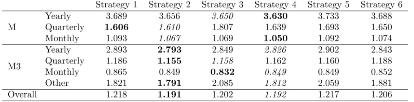
Similar insights are provided by Table 4, where the results from forecasting with ETS and evaluating on MASE are presented. The best strategy overall is still strategy 2, closely followed by strategy 4.
Table 4: Average MASE of the different forecasting strategies with ETS models and different data sets. Strategy 1 Strategy 2 Strategy 3 Strategy 4 Strategy 5 Strategy 6 M Yearly 3.689 3.656 3.650 3.630 3.733 3.688 Quarterly 1.606 1.610 1.807 1.639 1.693 1.650 Monthly 1.093 1.067 1.069 1.050 1.092 1.074 M3 Yearly 2.893 2.793 2.849 2.826 2.902 2.843 Quarterly 1.186 1.155 1.158 1.162 1.160 1.188 Monthly 0.865 0.849 0.832 0.849 0.849 0.852 Other 1.821 1.791 2.085 1.812 2.059 1.881 Overall 1.218 1.191 1.202 1.192 1.217 1.206
The same analysis was performed by replacing ETS as the underlying model with ARIMA automatic modelling. It should be noted that this analysis expands the original study by Bergmeir et al. (2016) where only exponential smoothing models were considered. The re-sults are presented in Tables 5 and 6. Rere-sults for strategy 2 (model combination benchmark) are not presented for ARIMA, as there exists an infinite number of ARIMA models.
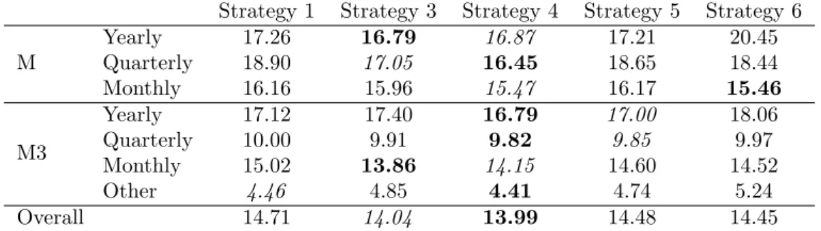
By comparing strategy 3 (bagging) with strategy 1 (benchmark; simple model selection), we can conclude that bagging for time series forecasting is beneficial for ARIMA modelling as well. In fact, the overall gains in performance are even higher than in the case of ETS, at 4.6% for sMAPE and 2.9% for MASE. The performance improvements of bagging over traditional model selection seem to be even more consistent in the time series where seasonality might appear (quarterly or monthly data).
Strategy 4 (bootstrap model selection) offers the best performance overall, being bet-ter than strategy 3 for both sMAPE and MASE. Inbet-terestingly, strategy 4 outperforms the benchmark in 7 out of 7 subsets of data for the sMAPE and in 6 out of 7 subsets for the MASE. Moreover, strategy 4 is ranked first or second for all subsets. The superior
perfor-Table 5: Average sMAPE (%) of the different forecasting strategies for ARIMA models and different data sets.
Strategy 1 Strategy 3 Strategy 4 Strategy 5 Strategy 6 M Yearly 17.26 16.79 16.87 17.21 20.45 Quarterly 18.90 17.05 16.45 18.65 18.44 Monthly 16.16 15.96 15.47 16.17 15.46 M3 Yearly 17.12 17.40 16.79 17.00 18.06 Quarterly 10.00 9.91 9.82 9.85 9.97 Monthly 15.02 13.86 14.15 14.60 14.52 Other 4.46 4.85 4.41 4.74 5.24 Overall 14.71 14.04 13.99 14.48 14.45
Table 6: Average MASE of the different forecasting strategies for ARIMA models and different data sets. Strategy 1 Strategy 3 Strategy 4 Strategy 5 Strategy 6
M Yearly 3.474 3.453 3.434 3.482 4.210 Quarterly 1.801 1.758 1.675 1.829 1.794 Monthly 1.164 1.112 1.094 1.162 1.149 M3 Yearly 2.964 2.927 2.856 2.904 3.290 Quarterly 1.186 1.161 1.157 1.163 1.206 Monthly 0.877 0.829 0.848 0.852 0.907 Other 1.832 2.094 1.847 2.029 2.434 Overall 1.246 1.210 1.200 1.233 1.318
mance of strategy 4 suggests that most of the gains of bagging for time series forecasting derive from the fact that the bootstraps may select different models (i.e., model uncertainty). The results obtained by strategies 5 and 6 with ARIMA models contradict the corre-sponding results with ETS models. Strategy 5, which deals with data uncertainty, shows some improvements over the benchmark. In any case, the overall improvements are smaller than those obtained by strategies 3 and 4. On the other hand, strategy 6 is ranked last based on MASE and second to last based on sMAPE. Its performance is especially poor for the yearly and other data. Overall, we can say that strategies 5 and 6 provide mixed results, which seem to depend upon the forecasting family of models applied (ETS or ARIMA) and the number of parameters to be estimated.
4.3. The impact of time series length
We also examined the impact of the in-sample length of each series (number of avail-able observations) on the performance of bagging (strategy 3) over the simple benchmark (conventional model selection; strategy 1). To this end, we calculated the per series percent-age improvement of strategy 3 (S3) over strategy 1 (S1) as improvement = 1001− EMS3
EMS1
, whereEM refers to the sMAPE or MASE for that particular time series. This was regressed on the number of observations of each series, improvement = b0 +b1 ×length. We fitted such models for all bagging/bootstrapping approaches in this study (strategies 3 to 6), for both automatic forecasting methods (ETS and ARIMA), for both error measures (sMAPE and MASE), and for all frequencies (yearly, quarterly, monthly and other) pooling together
series of the same frequency from the M and M3 competitions. Table 7 reports the values of the b1 coefficients when a significant relationship is observed (p≤0.05).
Table 7: The average impact of one additional observation on the percentage improvement of the different bagging approaches over the simple benchmark, strategy 1.
ETS ARIMA
sMAPE MASE sMAPE MASE
Strategy 3 Yearly - - - -Quarterly - - - -Monthly - - - -Other - - - -Strategy 4 Yearly - - - -Quarterly -0.1491 - - -Monthly - - -0.0673 -0.0773 Other - - - -Strategy 5 Yearly - - - -Quarterly - - -0.2601 -0.2831 Monthly - - - -Other - - - -Strategy 6 Yearly - - 1.7792 1.5981 Quarterly - - 0.9473 0.8723 Monthly - - -0.1533 -0.1503 Other - - 4.1892 4.3582
1statistically significant at level 0.05 2statistically significant at level 0.01 3statistically significant at level 0.001
The relative performance of strategy 3 over strategy 1 is not influenced by the length of series. Similarly, when ETS is the estimator, the impact of length is not significant in almost all cases; the only exception is the performance of strategy 4 over strategy 1 as measured by sMAPE for the quarterly data, where an additional year of data (four quarters) results in an 0.6% decrease on average. When ARIMA is considered as the estimator, there are a few cases where the relationship seems to be significant. Most interestingly, the sMAPE of the bootstrap parametrisation approach (strategy 6) for the yearly frequency improves by 1.8% on average relative to the sMAPE of strategy 1 for each additional observation of data. The respective improvements for the quarterly data appear to be 3.8% for each additional year of data. Overall, we can say that when a significant relationship exists, its impact and direction depends on the frequency and the strategy under investigation.
4.4. Results based on the CBB and the LPB
Apart from the MBB for bootstrapping the remainder of the series, we additionally considered two more approaches: CBB and LPB. Appendix A presents the ranks of each strategy for the three bootstrap approaches, MBB, CBB and LPB. For example, “4-3-4” of M-Monthly data and strategy 3 in Table A.8 suggests that it is ranked fourth, third and fourth when MBB, CBB and LPB were applied respectively. In general, we observe consistency across the ranks, which suggests that the insights obtained from applying MBB
hold when other approaches are used to bootstrap the remainder. Any differences, such as those observed for the M3-Quarterly data in Table A.8, are due to the fact that the respective strategies perform on very similar levels. Additionally, it is worth mentioning that strategy 4 (boostrap model combination) overall outranks strategy 2 (model combination benchmark) for LPB (both error measures, sMAPE and MASE) and CBB (MASE).
5. Discussion and implications
Forecasting is a crucial component for different departments of a company, including but not limited to sales, marketing, finance, operations, procurement and human resources. Given the plethora of available forecasting models, selecting the one that best extrapolates the past historical data has been considered as the holy grail of forecasting (Petropoulos et al., 2014). Even if the best model form has been correctly identified, the selection of the optimal parameters can still be challenging. Bagging for time series forecasting (Bergmeir et al., 2016) attends to these challenges by exploiting bootstraps of the original series and combining forecasts produced by potentially different models and sets of parameters. Our study focuses on decomposing the benefits of bagging for time series forecasting.
We empirically show that there is little to gain from considering different sets of param-eters of the forecasting models. This confirms and extends the results of a recent study on optimal versus suboptimal parameters for the simple exponential smoothing (SES) forecast-ing method. Nikolopoulos and Petropoulos (in press) showed that optforecast-ing for suboptimal values for the α smoothing parameter of SES results in out-of-sample performance that is insignificantly different to optimal values. Thus, savings on computational time can be con-sidered more important than the quest for parameters that are optimal for the in-sample but perform equally to suboptimal ones for the forecasting horizon. Such computational savings become even more relevant in the context where tens of thousands of time series have to be forecasted daily or even multiple times within a day, as is the case with retailers.
On the other hand, our results suggest that significant gains can be achieved if optimal combinations of different model forms are considered. In fact, by simply addressing the model uncertainty one can, on average, outperform bagging for time series forecasting. We suggest that such optimal weights can be derived by counting how many times each model form is selected as optimal when fitting bootstraps of the original data. We call this new combination approachbootstrap model combination. The bootstrap model combination per-forms similarly to the benchmark model combination based on information criteria, however the latter has the disadvantage that it cannot be applied in the cases where the pool of models is not finite (as is the case in the ARIMA family of models) or when models from different families are considered.
While our study focuses on two families of forecasting models (ETS and ARIMA) where model selection is performed within each family based on information criteria, one could also consider an application of the bootstrap model combination using cross-validation tech-niques. In such a scenario, the forecasting models to select from may not be restricted to a single family. The performance of each model is measured through a rolling origin eval-uation on a set of hidden data (Tashman, 2000). Subsequently, the model with the best
performance is selected (Fildes and Petropoulos, 2015). This process is repeated for the original series and the bootstraps, allowing the calculation of combination weights across all available models.
The implications of our study are significant both in terms of theory and practice. First, we demonstrate the origin of the benefits of bagging for time series forecasting. Second, we contribute to the discussion of forecast combinations with the use of optimal weights. Third, we believe that our study provides suggestions for the efficient design of forecasting support systems and, in particular, the refinement of algorithms for automatic time series forecasting. Finally, even if we do not consider forecast uncertainty explicitly and we do not compare the corresponding prediction intervals of the ETS and automatic ARIMA versus the proposed strategies, we believe that our study contributes to the research on decision making un-certainty and more specifically decisions related to selecting forecasting models. Automatic model recommendations by leading software are often reviewed (and judgmentally adjusted) by demand planners and managers. Bagging and bootstrapping model combination provide more robust forecasts, efficiently tackling model uncertainty. By rendering this selection and combination process transparent (for example, by reporting the composition of the selected forecasts, such as 60% ETS(A,N,N), 28% ETS(A,A,N) and 12% ETS(M,A,M)), it is likely to lead to increased trust and acceptance of the software automatic forecast.
Improving the forecast accuracy of well-established and state-of-the-art automatic algo-rithms, such as ETS and ARIMA (Hyndman and Khandakar, 2008), has significant impli-cations to improved inventory decisions as well. A lower forecast error will inevitably lead to lower safety stocks which in turn can be translated to reduced inventory holding and/or increased customer service levels. As Syntetos et al. (2010) suggest, even the smallest gains in accuracy (of about 1%) may be translated to considerable inventory reductions (approx-imately 15-20%) coupled with higher fill-rates. Apart from ordering and replenishment, accurate forecasting and demand uncertainty can influence various optimisation problems, such as healthcare management (Ahmadi-Javid et al., 2017, “forecasting techniques are a cornerstone for most outpatient appointment system decisions”), strategic capacity plan-ning and technology choice decisions (Jakubovskis, 2017) and retail promotional planplan-ning and optimisation with a target to maximise profits (Ma and Fildes, 2017).
However, for such gains to materialise, the proposed strategies should be directly appli-cable to practice. The open source forecastpackage (currently in its 8.2 version) for the R statistical language provides implementations of ETS and automatic ARIMA approaches, which were considered the benchmarks (strategy 1) in our study. Moreover, there is evidence that suggests that this package is very widely used in corporate practice:
• The package averages 79,000 downloads per month.2
• As of Dec 28, 2018, the DataCamp course on the package has had over 8,400 partici-pants.3
• As of Dec 28, 2018, there are 2,410 search results on stackoverflow for the package.4
2https://www.rdocumentation.org/packages/forecast/versions/8.1 3https://www.datacamp.com/courses/forecasting-using-r
Since version 8.0, theforecastpackage also includes strategy 3 for ETS (bagging, function baggedETS()). A future version of the forecast package will feature a function that implements strategy 4, bootstrap model combination.
Finally, we would like to make a note on the computational cost of producing forecasts using the approaches described in this study. Even if bagging and bootstrap model combi-nation approaches are computationally more expensive as they involve the fitting of optimal models for multiples of the original series, they provide performance improvements that are likely to pay off. Moreover, less than 99 bootstraps might be considered; as Petropoulos (2014) suggests, the improvements of bagging for time series seem to taper off after 50 bootstraps.
6. Conclusions
Bagging for time series forecasting considers the application of automatic forecasting on multiple time series (the original one and the bootstraps) and the combination of those forecasts. The bootstraps are produced via decomposing the Box-Cox transformed original data, and performing random sampling on the remainder, maintaining the trend and seasonal components intact. Bagging has shown considerable benefits in forecast accuracy (Bergmeir et al., 2016). In this study, we confirmed the superior performance of bagging on more data, different forecasting models and different bootstraps, and we developed some computational methods to analyse where these gains originate from.
We suggested that bagging performs well as it can simultaneously tackle the three sources of uncertainty. Data uncertainty refers to the variation of the inherent random component that exists in any time series. Model uncertainty refers to the uncertainty linked with the selection of the ‘optimal’ model form. Parameter uncertainty refers to the selection of the set of parameters that best describes the observed and unobserved data. Bootstrapping naturally tackles the data uncertainty. Fitting different models to each bootstrap series ad-dresses the model uncertainty dimension. Even if a single model form is identified as optimal across all bootstraps, different sets of parameters will apply, thus tackling the uncertainty in identifying the optimal set of parameters.
We proposed three strategies where the potential benefits of bagging for each one of these sources of uncertainty are considered separately. We benchmarked these strategies against simple model selection, model combination using weights based on information criteria and bagging. We showed that if one focuses on just tackling the model uncertainty then ben-efits equal to that of bagging, if not greater, are recorded. Tackling the other sources of uncertainty would decrease the forecast error for some subsets and frequencies, but not for all. Overall, we recommend the bootstrap model combination where optimal model forms are identified from the bootstraps and these are then fitted to the original data. A weighted combination across the forecasts produced from different model forms should reflect the frequency with which each model form is identified as optimal amongst the bootstrap series. This study focused on investigating the performance benefits when only one source of uncertainty is tackled at each time. A possible path for future research would be the inves-tigation of strategies when two out of three sources are tackled together. Also, it would be
interesting to see how bagging or bootstrap model selection are influenced by the number of bootstraps produced (how many bootstraps are enough to achieve convergence) and the average operators applied for combination (arithmetic mean versus median versus mode).
References
Ahmadi-Javid, A., Jalali, Z., Klassen, K. J., 2017. Outpatient appointment systems in healthcare: A review of optimization studies. European Journal of Operational Research 258 (1), 3–34.
Bergmeir, C., Hyndman, R. J., Ben´ıtez, J. M., 2016. Bagging exponential smoothing methods using STL decomposition and Box-Cox transformation. International Journal of Forecasting 32, 303–312.
Box, G. E. P., Cox, D. R., 1964. An analysis of transformations. Journal of the Royal Statistical Society, Series B 26 (2), 211–252.
Box, G. E. P., Draper, N. R., 1987. Empirical Model-Building and Response Surfaces. John Wiley & Sons, New York.
Breiman, L., 1996. Bagging predictors. Machine Learning 24 (2), 123–140. B¨uhlmann, P., 1997. Sieve bootstrap for time series. Bernoulli 3 (2), 123–148.
Cleveland, R. B., Cleveland, W. S., McRae, J. E., Terpenning, I., 1990. STL: A seasonal-trend decomposition procedure based on loess. Journal of Official Statistics 6, 3–73.
Cleveland, W. S., Grosse, E., Shyu, W. M., 1992. Local regression models. Statistical Models in S. Chapman & Hall/CRC, Ch. 8.
Cordeiro, C., Neves, M., 2009. Forecasting time series with BOOT.EXPOS procedure. REVSTAT - Statis-tical Journal 7 (2), 135–149.
Fildes, R., Petropoulos, F., 2015. Simple versus complex selection rules for forecasting many time series. Journal of Business Research 68 (8), 1692–1701.
Guerrero, V. M., 1993. Time-series analysis supported by power transformations. Journal of Forecasting 12, 37–48.
Hastie, T., Tibshirani, R., Friedman, J., 2009. The Elements of Statistical Learning: Data Mining, Inference, and Prediction. Springer.
Hyndman, R. J., 2017. forecast: Forecasting functions for time series and linear models. R package version 8.0.
URLhttp://github.com/robjhyndman/forecast
Hyndman, R. J., Athanasopoulos, G., 2014. Forecasting: principles and practice. OTexts, Melbourne, Aus-tralia.
URLhttp://otexts.com/fpp/
Hyndman, R. J., Khandakar, Y., 2008. Automatic time series forecasting: The forecast package for R. Journal of Statistical Software 27 (3), 1–22.
Hyndman, R. J., Koehler, A. B., 2006. Another look at measures of forecast accuracy. International Journal of Forecasting 22 (4), 679–688.
Jakubovskis, A., 2017. Strategic facility location, capacity acquisition, and technology choice decisions under demand uncertainty: Robust vs. non-robust optimization approaches. European Journal of Operational Research 260 (3), 1095–1104.
Kolassa, S., 2011. Combining exponential smoothing forecasts usingAkaike weights. International Journal of Forecasting 27 (2), 238–251.
K¨unsch, H. R., 1989. The jackknife and the bootstrap for general stationary observations. Annals of Statistics 17 (3), 1217–1241.
Ma, S., Fildes, R., 2017. A retail store SKU promotions optimization model for category multi-period profit maximization. European Journal of Operational Research 260 (2), 680–692.
Makridakis, S., Andersen, A., Carbone, R., Fildes, R., Hibon, M., Lewandowski, R., Newton, J., Parzen, E., Winkler, R., 1982. The accuracy of extrapolation (time series) methods: Results of a forecasting competition. Journal of Forecasting 1 (2), 111–153.
Makridakis, S., Hibon, M., 2000. The M3-competition: Results, conclusions and implications. International Journal of Forecasting 16 (4), 451–476.
McMurry, T., Politis, D. N., 2010. Banded and tapered estimates of autocovariance matrices and the linear process bootstrap. Journal of Time Series Analysis 31, 471–482.
Nikolopoulos, K., Petropoulos, F., in press. Forecasting for big data: does sub-optimality matter? Computers & Operations Research.
Petropoulos, F., 2014. Guest post: On the robustness of bagging exponential smoothing. Nikolaos Kourentzes, Forecasting Research Blog.
URLhttp://kourentzes.com/forecasting/2014/10/31/
Petropoulos, F., Makridakis, S., Assimakopoulos, V., Nikolopoulos, K., 2014. ‘Horses for Courses’ in demand forecasting. European Journal of Operational Research 237, 152–163.
Politis, D. N., Romano, J. P., 1991. A circular block-resampling procedure for stationary data. Tech. rep. No. 370, Department of Statistics, Stanford University, Stanford, California, USA.
R Core Team, 2017. R: A Language and Environment for Statistical Computing. R Foundation for Statistical Computing, Vienna, Austria.
URLhttp://www.R-project.org/
Syntetos, A. A., Nikolopoulos, K., Boylan, J. E., 2010. Judging the judges through accuracy-implication metrics: The case of inventory forecasting. International Journal of Forecasting 26 (1), 134–143.
Tashman, L. J., 2000. Out-of-sample tests of forecasting accuracy: An analysis and review. International Journal of Forecasting 16 (4), 437–450.
Appendix A. Ranks of the different bootstrapping approaches: MBB, CBB and LPB.
Table A.8: Ranks of the three bootstrapping approaches in terms of sMAPE (%) for the different forecasting strategies for ETS models. For example, “1-3-2” denotes that for that particular data set, a strategy was ranked first, third and second when MBB, CBB and LPB were applied respectively.
Strategy 1 Strategy 2 Strategy 3 Strategy 4 Strategy 5 Strategy 6 M Yearly 5-5-5 4-4-4 3-1-2 1-2-1 6-6-6 2-3-3 Quarterly 2-2-2 3-3-3 6-6-6 1-1-1 5-5-5 4-4-4 Monthly 5-5-5 1-2-2 4-3-4 2-1-1 6-6-6 3-4-3 M3 Yearly 5-6-4 2-2-1 4-4-6 6-3-2 3-5-5 1-1-3 Quarterly 4-4-5 1-1-1 6-6-4 2-2-2 3-3-6 5-5-3 Monthly 6-6-6 3-3-3 1-1-1 2-2-2 5-5-5 4-4-4 Other 2-2-2 1-1-1 6-6-6 3-3-3 5-5-5 4-4-4 Overall 5-5-5 1-1-2 3-3-3 2-2-1 6-6-6 4-4-4
Table A.9: Ranks of the three bootstrapping approaches in terms of MASE for the different forecasting strategies for ETS models. For example, “1-3-2” denotes that for that particular data set, a strategy was ranked first, third and second when MBB, CBB and LPB were applied respectively.
Strategy 1 Strategy 2 Strategy 3 Strategy 4 Strategy 5 Strategy 6 M Yearly 5-5-5 3-3-3 2-1-1 1-2-2 6-6-6 4-4-4 Quarterly 1-1-1 2-2-2 6-6-6 3-3-3 5-5-5 4-4-4 Monthly 6-5-6 2-2-3 3-3-2 1-1-1 5-6-5 4-4-4 M3 Yearly 5-5-4 1-1-2 4-4-3 2-2-1 6-6-6 3-3-5 Quarterly 5-6-6 1-3-3 2-1-1 4-2-2 3-4-4 6-5-5 Monthly 6-6-6 3-2-3 1-1-1 2-3-4 4-5-5 5-4-2 Other 3-3-3 1-1-1 6-6-6 2-2-2 5-5-5 4-4-4 Overall 6-5-5 1-2-2 3-3-3 2-1-1 5-6-6 4-4-4
Table A.10: Ranks of the three bootstrapping approaches in terms of sMAPE (%) for the different forecasting strategies for ARIMA models. For example, “1-3-2” denotes that for that particular data set, a strategy was ranked first, third and second when MBB, CBB and LPB were applied respectively.
Strategy 1 Strategy 3 Strategy 4 Strategy 5 Strategy 6 M Yearly 4-4-4 1-1-1 2-2-2 3-3-3 5-5-5 Quarterly 5-5-5 2-2-2 1-1-1 4-4-4 3-3-3 Monthly 4-5-3 3-3-5 2-1-2 5-4-4 1-2-1 M3 Yearly 3-3-2 4-4-4 1-1-1 2-2-3 5-5-5 Quarterly 5-5-5 3-2-2 1-1-1 2-3-3 4-4-4 Monthly 5-5-5 1-1-1 2-2-2 4-4-4 3-3-3 Other 2-2-2 4-4-4 1-1-1 3-3-3 5-5-5 Overall 5-5-5 2-2-2 1-1-1 4-4-3 3-3-4
Table A.11: Ranks of the three bootstrapping approaches in terms of MASE for the different forecasting strategies for ETS models. For example, “1-3-2” denotes that for that particular data set, a strategy was ranked first, third and second when MBB, CBB and LPB were applied respectively.
Strategy 1 Strategy 3 Strategy 4 Strategy 5 Strategy 6 M Yearly 3-4-4 2-2-2 1-1-1 4-3-3 5-5-5 Quarterly 4-4-3 2-2-2 1-1-1 5-5-5 3-3-4 Monthly 5-4-4 2-2-2 1-1-1 4-5-5 3-3-3 M3 Yearly 4-4-4 3-3-2 1-1-1 2-2-3 5-5-5 Quarterly 4-4-4 2-2-2 1-1-1 3-3-3 5-5-5 Monthly 4-4-4 1-1-1 2-2-2 3-3-3 5-5-5 Other 1-1-2 4-4-4 2-2-1 3-3-3 5-5-5 Overall 4-4-4 2-2-2 1-1-1 3-3-3 5-5-5