R E S E A R C H
Open Access
Characterisation of survivability resilience
with dynamic stock interdependence in
financial networks
Junqing Tang
*, Layla Khoja and Hans R. Heinimann
*Correspondence: [email protected] ETH Zurich, Future Resilient Systems, Singapore-ETH Centre, 1 CREATE Way, CREATE Tower, Singapore 138602, Singapore
Abstract
This paper examines the dynamic evolutionary process in the London Stock Exchange and uses network statistical measures to model the resilience of stock. A large historical dataset of companies was collected over 40 years (1977-2017) and conceptualised into weighted, temporally evolving and signed networks using correlation-based
interdependences. Our results revealed a “fission-fusion” market growth in network topologies, which indicated the dynamic and complex characteristics of its evolutionary process. In addition, our regression and modelling results offer insights for construction a “characterisation tool” which can be used to predict stocks that have delisted and continuing performance relatively well, but were less adequate for stocks with normal performance. Moreover, the analysis of deviance suggested that the survivability resilience could be described and approximated by degree-related centrality measures. This study introduces a novel alternative for looking at the bankruptcy in the stock market and is potentially helpful for shareholders, decision- and policy-makers.
Keywords: Survivability resilience, Financial stock networks, Network dynamic evolution, Weighted mtultinomial logistic regression
Introduction
Complex network approaches are commonly applied in a wide range of academic fields (Barabási 2016; Münnix et al. 2012), and studies on network topology have always been an interesting topic. The statistical measures of topology and interdependence are often strongly associated with the performance of network components. For exam-ple, in financial stock networks, the correlation-based topology varies with the different condition of nodes (stocks) and edges (correlation-based interdependence). Here, we investigated such associations and tried to establish a predictive relationship between net-work measures and a special type of component performance, survivability resilience, in correlation-based stock networks.
As self-explained, the term survivability resilience describes the ability of the subject to survive, to be reliable, and to avoid failure in the environment (Singpurwalla1995). It answers the question of how resilient the subject is in a static or dynamic envi-ronment to maintain long survival (Sterbenz et al. 2010). In the stock market, the survivability is termed to illustrate the ability of stocks/listed firms to prevent corporate
failure/bankruptcy or being delisted from the market. Categorising and predicting cor-porate failure is essential in bankruptcy studies (Khoja et al.2016) because it is of great importance in providing early warnings about a company’s financial distress to stakehold-ers, business managstakehold-ers, policy-makstakehold-ers, and financial economists (Amendola et al.2017; Jones et al.2017) and it is hard to be characterised and predicted (Allen and Babus2009). Over the past 50 years, various statistical models based on financial or accounting data have been applied for predicting corporate bankruptcy (du Jardin et al.2017). The most frequently used methods for studying stock survivability include genetic fuzzy models (Kuo et al. 2001), artificial networks (Zhang et al. 1999), genetic algorithms (Zelenkov et al.2017), and neural networks and deep learning networks (Ticknor2013; Chong et al.2017). Other traditional statistical models have also been proposed, such as multivariate discriminant analysis and logistic regression (Beaver1966; Altman1968; Shumway2001; Mossman et al.1998; Lee et al.1996). In recent years, machine learning models have been popular in bankruptcy predictions due to their excellent performance on accuracy (Barboza et al.2017). However, the majority of those models require a sub-stantial amount of accounting-related data (from a company’s financial statement) as input variables (du Jardin et al.2017). This sometimes leads to an unpromising issue as those accounting data could not always be available in hand. Furthermore, most studies of bankruptcy have concentrated on only failed firms and overlooked the possibility of using networks perspectives to model stocks/firms with different survivability, including those of exceptionally resilient performance.
On the other hand, apart from bankruptcy literature, studies of financial stock networks themselves are not rare in the literature. One interesting topic is to study the temporal transformation of the market with a network perspective. The special swarm patterns caused by different stock’s survivability performance often manifest in the network evo-lution process. However, most of the previous works have only briefly discussed such process of their studied networks (Bonanno et al.2004; Mantegna1999; Onnela et al. 2003), and most have been based only on either a short time period or a small fraction of the market population (Huang et al.2009; Gao et al.2013). We believe that studying the long-term evolutionary process of the market networks would help us understand more about the survivability resilience of stocks.
Thus, the two-fold purposes of this paper are: (a) firstly, to explore the correlation-based interdependence of a whole market by constructing weighted, signed and temporal stock networks and to understand the long-term dynamic evolution of their topological features; and (b) with the understandings of long-term historical evolution process from the first purpose, we then characterise the survivability resilience of stocks via statisti-cal models (using interdependence and network measures as variables) and then explore their predictive strengths by identifying highly descriptive parameters. This work is an expanded version of preliminary work in (Tang et al.2017). Here we expanded the scopes by using a new and more completed dataset and applying new modelling approaches. Also, we tested and validated the predictability of the model and studied its performance regarding various stock behaviours.
analysis are presented. “Survivability and resilience characterisation” section consists detailed results and discussion on survivability resilience, followed by final conclusions summarised in “Conclusion” section.
Data and methodology
We used DataStreamTM to gather historical data on the daily closing stock prices (adjusted stock price, which accounts for actions such as splits and dividends) for 7206 companies that had ever traded or were still trading on the London Stock Exchange over a 40-year period (total of 10438 trading days), from 04/05/1977 to 05/05/2017.
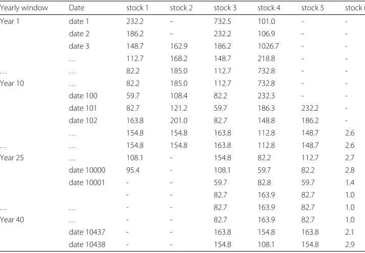
Firstly, we categorised all stocks before constructing networks. The categorisation of Delisted companies and Continuing companies were based upon their ability to survive in the markets. Stocks that did not belong to either of those two groups were treated as Normal companies. The following definitions were used for our categories:
• Delisted stocks(example stocks 1 and 2 in Table1): those companies that were delisted when they have a high leverage generally because they were unprofitable, and/or were facing difficulties in gaining additional equity capital during their public life (Pour and Lasfer2013). Consequently, those companies have been delisted to become privately owned companies, acquired companies or in some cases, went bankrupt.
• Continuing stocks(example stocks 3 and 4 in Table1): those companies have good opportunities for investment growth, and which showed increases in equity capital when quoted in the market (Pour and Lasfer2013). For our purpose, continuing group represents the companies which have been continuing to trade in the market for the entire 40-years observation period.
Table 1Structures for three groups of collected data
Yearly window Date stock 1 stock 2 stock 3 stock 4 stock 5 stock 6
Year 1 date 1 232.2 - 732.5 101.0 -
-date 2 186.2 - 232.2 106.9 -
-date 3 148.7 162.9 186.2 1026.7 -
-. -. -. 112.7 168.2 148.7 218.8 -
-. -. -. . . . 82.2 185.0 112.7 732.8 -
-Year 10 . . . 82.2 185.0 112.7 732.8 -
-date 100 59.7 108.4 82.2 232.3 -
-date 101 82.7 121.2 59.7 186.3 232.2
-date 102 163.8 201.0 82.7 148.8 186.2
-. -. -. 154.8 154.8 163.8 112.8 148.7 2.6
. . . 154.8 154.8 163.8 112.8 148.7 2.6
Year 25 . . . 108.1 - 154.8 82.2 112.7 2.7
date 10000 95.4 - 108.1 59.7 82.2 2.8
date 10001 - - 59.7 82.8 59.7 1.4
- - 82.7 163.9 82.7 1.0
. . . - - 82.7 163.9 82.7 1.0
Year 40 . . . - - 82.7 163.9 82.7 1.0
date 10437 - - 163.8 154.8 163.8 2.1
date 10438 - - 154.8 108.1 154.8 2.9
• Normal stocks(example stocks 5 and 6 in Table1): those companies were initially listed at some point during the observation period and had not failed yet by the end of the observation period.
Next, we determined the edges of these complex financial networks, based on prede-fined interdependence that characterised a certain relationship or interaction between acting nodes. A considerable number of studies have focused on methods for constructing the edges in stock networks. They include the minimal spanning tree (Bonanno et al. 2003; Vandewalle et al. 2001; Kwapie´n et al. 2017), planar maximally filtered graph (Tumminello et al.2005), threshold filtering mechanism (Huang et al.2009), and winner-takes-all approach (Chi et al.2010). Other more recent investigations have concentrated on the methods for constructing interdependence, e.g., Pearson correlation coefficients (Heiberger 2014), Partial correlation coefficients (Xu et al. 2017), Pearson product-moment correlation coefficient (Zhang et al.2017), covariance and Gaussian graphical models (Xuan and Murphy2007). Generally speaking, the Pearson correlation coefficient tends to be the most widely applied methods.
Therefore in our study, we used the Pearson correlation coefficients to construct net-works, using pair-wise logarithmic returns for stocks on a daily basis. For this, we letri(t)
andpi(t) denote the log-return and closing price of stockiat timet, respectively. The
daily log-return can be expressed as follows:
ri(t)=ln
pi(t)
−lnpi(t−t)
(1)
where t is one trading day,t = 1. Then we write Pearson correlation coefficients (Benesty et al.2009)ci,jbetween stockiandjas:
ci,j= <
ri(t)×rj(t) >−<ri(t) >×<rj(t) >
σi×σj
(2)
where < . >indicates the mean value andσi is the standard deviation of the stock i
in a time series. Thep-values were also computed for each coefficient and used as the threshold to prune the networks and filter out those insignificant correlations. In order to avoid severe topological information loss while pruning the edges (according to the evidence shown in Huang et al. (2009), the edge density of stock network drops sharply fromci,j=0.1), we setp-value threshold as 0.01 to eliminate weak correlations for−0.1<
ci,j < 0.1, replacing them with “0”. We then used the coefficient values as edge weights
to represent the intensity of connections. Like the positive/negative interactions in social networks (Leskovec et al.2010), we also showed considerations to negative signs in the correlation-based financial networks, and the edge signs were same as the corresponding signs of those coefficients.
“NAN” from a certain row, all rows with value “NAN” were omitted and only the common section was used to calculate the coefficient.
Understanding interdependence
In this section, we investigate the basic network information extracted from the stock networks and study the dynamic evolution of correlation-based interdependence in long-term observation.
Network topology
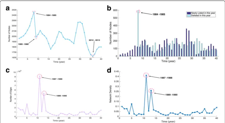
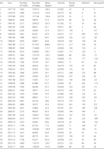
The growth of networks shows a constant fluctuation in terms of the total number of nodes (Fig.1a), the number of newly listed and delisted nodes (Fig.1b), the number of edges (Fig.1c), and the network density (Fig.1d). Counterintuitively, the networks did not evolve constantly as the market population gradually increased. Subplot (a) presents three major shrinkages and expansions of the market population (Table2). The first continuous increment occurred during the first eight years when the number of total nodes increased from 1963 to 2336. However, between 1984 and 1986, numerous stocks (599) were de-listed due to a severe recession in the UK in the early 1980s. This was followed by an increasing number of bankruptcy cases (Rhim1993).
The second expansion was found in 1992 to 1993 (16th year), when the market grew from 1760 stocks to 2093 in 1996-1997 (20th year), after that the number gradually decreased again until 2003-2004. In the following two years (28th, 2004-2005 and 29th, 2005-2006), the market rapidly expanded. However, from the 30th year (2006-2007), the market rapidly downsized to 1627 stocks in 2012-2013. This trend is even more apparent in subplot (b), which shows the rise and fall in the number of newly listed and delisted stocks. It is interesting that a major network synchronisation existed in the number of edges (see subplot (c)), where a dramatic change in the number of nodes did not necessar-ily lead to a similar change in the number of edges. This synchronisation during a period of massive shrinkage might have, in fact, improved the correlations between stock pairs,
Table 2Statistic summary of 40 constructed networks
No. Year Number
of nodes
Number of edges
Mean degree
Density Newly listed
Delisted Net growth
1 1977-78 1963 192913 196.5 0.1002 22 13 9
2 1978-79 1986 152314 153.4 0.0773 36 9 27
3 1979-80 2010 157144 156.4 0.0778 33 2 31
4 1980-81 2056 58959 57.4 0.0279 48 10 38
5 1981-82 2121 283672 267.5 0.1262 75 10 65
6 1982-83 2200 60651 55.1 0.0251 89 3 86
7 1983-84 2336 32044 27.4 0.0117 139 2 137
8 1984-85 2461 82441 67.0 0.0272 127 599 -472
9 1985-86 1988 40221 40.5 0.0204 124 152 -28
10 1986-87 2039 45687 44.8 0.0220 202 138 64
11 1987-88 2113 917427 868.4 0.4112 217 199 18
12 1988-89 2049 114460 111.7 0.0546 144 150 -6
13 1989-90 2016 528287 524.1 0.2601 117 120 -3
14 1990-91 1964 127319 129.7 0.0660 68 140 -72
15 1991-92 1867 95383 102.2 0.0548 43 177 -134
16 1992-93 1760 70120 79.7 0.0453 71 87 -16
17 1993-94 1828 45818 50.1 0.0274 155 70 85
18 1994-95 1874 33363 35.6 0.0190 116 92 24
19 1995-96 1989 23959 24.1 0.0121 208 120 88
20 1996-97 2093 34956 33.4 0.0160 227 164 63
21 1997-98 2072 75287 72.7 0.0351 144 168 -24
22 1998-99 1988 67088 67.5 0.0340 87 202 -115
23 1999-00 1949 46248 47.5 0.0244 163 235 -72
24 2000-01 1949 39917 41.0 0.0210 236 173 63
25 2001-02 1934 72085 74.5 0.0386 158 135 23
26 2002-03 1900 49091 51.7 0.0272 100 183 -83
27 2003-04 1867 26718 28.6 0.0153 155 159 -4
28 2004-05 2069 34537 33.4 0.0161 361 139 222
29 2005-06 2267 37860 33.4 0.0147 337 189 148
30 2006-07 2273 98924 87.0 0.0383 194 189 5
31 2007-08 2242 103821 92.6 0.0413 157 192 -35
32 2008-09 2073 104141 100.5 0.0485 24 233 -209
33 2009-10 1874 55845 59.6 0.0318 34 196 -162
34 2010-11 1749 62130 71.0 0.0406 71 168 -97
35 2011-12 1656 105045 126.9 0.0767 75 106 -31
36 2012-13 1627 46304 56.9 0.0350 78 93 -15
37 2013-14 1667 46774 56.1 0.0337 134 70 64
38 2014-15 1758 55231 62.8 0.0358 161 92 69
39 2015-16 1800 116737 129.7 0.0721 135 96 39
40 2016-17 1802 145024 161.0 0.0894 98 78 20
Visualisation and basic features of dynamic evolution
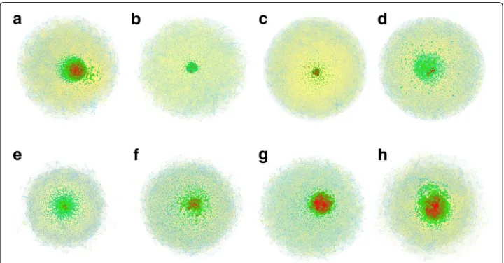
We usedGephiwith Fruchterman Reingold layout algorithm (Fruchterman and Reingold 1991) to visualise eight networks that roughly maintained an equal time gap. This algo-rithm is a famous member of a force-directed family, utilises nodes that are symbolised as solid objects and the edges acting as “springs” between them. By minimising the energy of the system, the algorithm moves the nodes and changes the forces between them until finally achieves an equilibrium state and then terminates.
Figure2shows the visualisation results for eight selected networks with an “atom-like” structure, wherein a few nodes were highly interconnected while the rest were sparsely connected around the core. Here, the color and the size of the nodes corresponded to their degree centrality, ranging from large red (high degree) via medium-green to small blue (low degree). Positive edges (positive correlation/interdependence) were indicated with yellow, and negative ones (negative correlation/interdependence), with light-blue. The thickness of the edges was proportional to their weights.
As can be seen, several high-degree nodes formed a core in each network, which indi-cated an uneven distribution of edges, i.e., nodes in the core area have a high tendency to connect with other high-degree nodes while nodes with fewer connections were more likely to be marginalised. We also determined that the core area (highly interconnected stocks) changed in size, possibly due to the “fission-fusion” evolving behaviour, which denotes a dynamic and unstable picture of interdependence among stocks.
In addition, most of the positive edges were concentrated around the core area while the negative edges were positioned toward the periphery, such as in subplots (a), (c), (d), (e), and (h). This interesting distribution of edge signs indicates that, in some years, the core stocks play influential roles as they not only positively interdependent with each other, but also have positive connections with other marginalised stocks. However, it also can be observed that this intriguing pattern does not stably last throughout the time.
For example, in subplots (b), (f ), and (g), it is difficult to observe aforementioned clear polarisation on the distribution of positive and negative edges around the core.
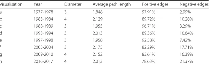
Table3shows some basic features of the corresponding networks. The small diame-ters (most of the networks have a diameter no greater than four) and small average path lengths (less than three) again verify a highly interactive and interdependent feature of the stock networks, which in addition denote a “small-world” effect. Taking a closer look at the percentage of edge signs in each network, we found that the ratio of positive and negative edges can be, although with fluctuations, approximated as 9:1, which indicated that a large number of the interdependence between stock pairs was positively correlated based on our network construction method. Such a high percentage of positive correla-tions could be one of the consequences of simultaneous market synchronisation under market crisis (Kauê Dal’Maso Peron et al.2012) (N.B. Because various methods exist for constructing correlation coefficient matrix, the pattern we observed here is inferred by applying Pearson correlation method. In other cases, such as using excess returns with Partial correlation coefficients, the percentage and distribution of the edge sign would be different, see an illustrative example of the year 2016-2017 in Appendix1. However, the comparative study on various methods is beyond the scope of this study. The interested readers can refer to Baba and Sibuya (2005); Kenett et al. (2010)).
Time-series network measures
Based on the understandings of the interdependence and features of topology evolu-tion obtained from the previous secevolu-tions, we then investigated the possibility of using more detailed network measures to characterise stocks with different survivability per-formance. In this way, we could determine which network measures could differentiate the stocks among different performance groups. Here, we excluded the flow- and route-oriented network measures, such as betweenness centrality and closeness centrality, because the flow and route choice are not issues in correlation-based networks.
The six selected network measures chosen for our review were: (1) Degree, k; (2) Strength,s; (3) Negative degree,k−; (4) Eigenvector centrality,e; (5) Clustering coeffi-cient (CC),c; and (6) Average neighbour degree (Ave. neighbour. degree),x. The selection criteria were based on the consideration of their popularity and universality in network literature. We also paid particular attention not only to the interdependence of a target node, but also to the condition of its neighbour nodes as well (i.e., eigenvector centrality, CC, and Ave. neighbour. degree). Here, we briefly explain them as follows (for interested readers, more details can be found Barabási (2016); Erciyes (2014); Newman (2010)).
Table 3Network statistics of illustrated networks
Visualisation Year Diameter Average path length Positive edges Negative edges
a 1977-1978 3 1.848 97.91% 2.09%
b 1983-1984 4 2.129 89.72% 10.28%
c 1988-1989 3 1.955 96.71% 3.29%
d 1993-1994 3 2.013 89.36% 10.64%
e 1997-1998 3 1.958 92.58% 7.42%
f 2003-2004 3 2.175 82.29% 17.71%
g 2009-2010 4 2.152 83.61% 16.39%
1 Node degreeis a straightforward nodal measure in complex networks, providing an indication of the importance of the node in terms of the number of its
neighbours. For an undirected network ofn nodes, the degreekiof nodei can be
expressed in an adjacency matrix as:
ki= n
j
Aij (3)
2 Yook et al. (2001) and Barrat et al. (2008) have studied theNode strengthsiof
network properties in weighted networks. This measure assesses the importance of a particular node in terms of its connection intensity. Node strength is defined as the sum of the weights on its total connections/degree. LetWijdenotes the edge
weight matrix corresponding to adjacency matrixAij, the strengthsican be
expressed as:
si= j
n
Wij (4)
3 In general, most existing network studies simply encode whether interdependence exist or not (Chiang et al.2014). The sign of the interdependence is normally neglected for topological simplification. However, the nodes with a large portion of negative interdependence might have some characters that of great interests for understanding the special features such as hidden community clusters (Ma and Zhang2018) and structure balance (Anchuri and Magdon-Ismail2012). Therefore, we gave equal attention to both positive andNegative degreein this paper to conceptualise our data as signed networks. It is important to notice that a negative edge literately represents the attribute of the edge as a negative relationship or opposite synchronisation, but does not indicate a low or an absent interaction between nodes. Instead, two nodes could be highly interactive and have a strong relationship with a negative edge (Newman2010). LetA−ij denote the negative correlation identified in an adjacency matrix, then:
k−i =
n
j
A−ij (5)
4 Eigenvector centralitycan be seen as an extension of the degree centrality but shows consideration to the relative importance of a node’s neighbours. This centrality measure, firstly proposed by Bonacich (1987), defines centralityeias
proportional to the sum of the centrality of neighbour nodes ofi, letκ1be the largest eigenvalue of matrixA, we have:
ei=
1 κ1
j
Aijej (6)
5 A very useful centrality measure for depicting the relation between pairs of nodes is known asClustering coefficient(CC), sometimes also referred to as transitivity. For each individual node, the CC is always defined as the local clustering
coefficient, which represents the average probability that a pair of nodei ’s neighbours are also connected (Newman2010).
ci=
number of pairs of is neighbour that are connected
6 The last one is a fairly straightforward measure of nodei ’s neighbourhood condition. TheAverage neighbour degree(Ave. neigh. degree) measures the average number of degree that connected toi ’s neighbours. Let i has n neighbours and their degree can be expressed askj, then:
xi=
n
j kj
n (8)
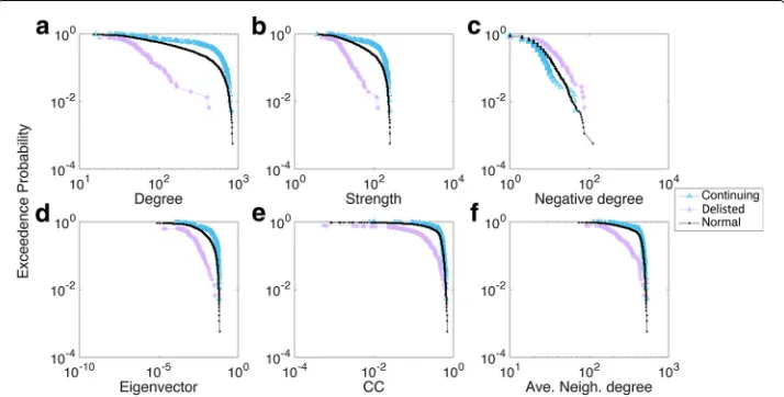
We calculated all six network measures for each stock in every stock group during the 40-year period. Using 1988-1989 as an example, Fig.3a-fillustrates the exceedance prob-ability distribution of network measures in the three groups. A clear gap existed between the Delisted group and the other two groups, indicating that the Delisted stocks behaved differently in terms of all six measures. However, the differences were not as easily spotted between the Continuing and Normal groups, except in the degree and strength distribu-tion plots (Fig.3a-b). We found it interesting that subplot (c) revealed a reverse order in the distribution of negative degree for a node, i.e., stocks from the Delisted group tended to have larger negative degrees when compared with stocks from the Continuing group, while Normal stocks fell in between.
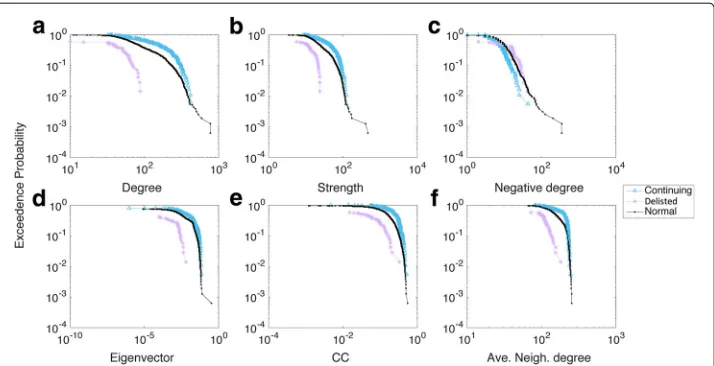
A similar tendency was found for other years, such as those seen from 1993 to 1994 (Fig. 4a-f). There, the negative degree distribution profile indicated some variations because the gaps among each group pair were not very obvious, and even some cross-ing and entanglement were found. However, the gaps between each pair of groups were generally clear and distinct, such as the significant difference noted in 2003-2004 (see Appendix 2). Thus, we confirmed that each group differed in terms of their network nodal features, thereby allowing us to use those differences as appropriate features when characterising the survivability performance of stocks within each group.
Survivability and resilience characterisation
In this section, survivability analysis based on aforementioned network measures are pre-sented. In order to study the possible relationship between stock survivability resilience and dynamic network measures, we constructed a model to characterise the different
Fig. 4Distribution of the six network measures in 1993-1994.aDegree;bStrength;cNegative degree;d Eigenvector;eCC;fAve. Neigh. degree
groups and explored the explanatory strength of each variable. The method applied here was selected as weighted multinomial logistic modelling. The particular reason for such selection is three-fold: First, we categorised all stocks into three nominal groups and that raises a problem of dealing with multi-class classification. Multinomial logistic regression is known to be suitable to handle dependent variable which has more than two levels. Sec-ond, because the populations of three groups were unbalanced in our data (a large portion of stocks are from the Normal group), we used penalised/weighted multinomial logistic regression to “re-balance” the groups by specifically assigning biased weights according to their actual number of observations. Third, as explained previously (Alaka et al.2017), the logistic-based classifiers have been shown to possess high transparency in understand-ing of detailed parameters. Even though their accuracy may not be as excellent as other popular machine-learning classifiers, their capability to facilitate decomposition analysis is still outstanding. Last but not the least, we had to consider that the regression could only show how the variation in predictive variables co-occurs with variation in response. There is no cause-and-effect relationship guaranteed between survivability resilience and nodal interdependence just based on regression analysis (Montgomery et al.2012).
Weighted multinomial logistic modelling
Multinomial logistic models depict the relationship between response probabilities and all six predictors, node degreeki, node strength si, negative degreeki−, eigenvectorei,
cluster coefficientciand average neighbour degreexi. By their very nature, such models
provide the estimated probability or odds of a target group against a reference group and, in our case, can be presented in the form as:
ln
α γ
=A+B×k+C×s+D×k−+E×e+F×c+G×x (9)
group and transformed the dependent variables into nominally distributed responses, where “1” represented the Delisted group, “2” was for the Continuing group, and “3” indicated stocks in the Normal group.
The data used to calibrate the models were network data from 1984-2012. The first seven years of networks, cross-referencing Fig.1b, were not used due to their extremely unbalanced number in the Delisted group (very low number of observations) and the last five years, 2012-2017, were selected to be used as testing sets in later sections. This left 28 networks, from 1984 to 2012, for model training and calibration. From there, we gained a total of 55903 observations, among which 4875 were in the Delisted group; 5096, in the Continuing group; and the remaining 45932 stocks, in the Normal group.
Before starting the model training, it takes only a moment’s reflection to realise that apart from two special groups (Delisted and Continuing) the majority of the population would, of course, be in the Normal group. The class imbalance problem, if left untreated, could have potentially biased the estimated calibration results and lose accuracy due to different distributions of each class. Treatments for such issue have always been a topic in statistics and machine learning communities (Mosley2013). There are several meth-ods are claimed as effective such as over-sampling, under-sampling, synthetic minority over-sampling technique (SMOTE) (Chawla et al. 2002) and threshold-moving meth-ods. Yet those methods have only been empirically observed as effective in most of the binary classifications, and a satisfactory solution for multi-class unbalance problem still needs investigation (Han et al.2011). Here, we applied penalised/weighted models for two aspects of consideration: First, the over-sampling and under-sampling approaches would have required random deletions or duplicate tuples in groups, which would have involved unavoidable manipulation of the original data. It also would have been difficult to decide which of the majority and minority groups to be under- and over-sampled, respectively. Second, because we had decided on a fixed model type and were unwilling to manipulate tuple data, a good alternative was to assign weights to bias the model, thereby giving more attention to the minority group. Furthermore, by not manipulating the data, our choice provided a different perspective on the problem by adjusting the models per se.
Each stock can be modelled with a penalised weight determined by its class group dur-ing the fittdur-ing process. Given a series of multi-class as 1,2,3,...i,. . .nin total, the weight for classican be determined as:
wi=
n
i=1Ni /n
Ni
(10)
whereNi is the number of observation in classi. In our case, the stocks in the Delisted
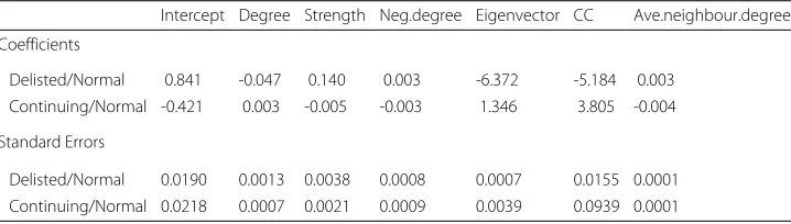
Table 4Estimated coefficients and corresponding standard errors
Intercept Degree Strength Neg.degree Eigenvector CC Ave.neighbour.degree
Coefficients
Delisted/Normal 0.841 -0.047 0.140 0.003 -6.372 -5.184 0.003
Continuing/Normal -0.421 0.003 -0.005 -0.003 1.346 3.805 -0.004
Standard Errors
Delisted/Normal 0.0190 0.0013 0.0038 0.0008 0.0007 0.0155 0.0001 Continuing/Normal 0.0218 0.0007 0.0021 0.0009 0.0039 0.0939 0.0001
In addition, we tested the significance of the estimated coefficients. We firstly per-formed a two-tailed z test. Table 5 indicates that all estimated coefficients were very significant for estimation on both groups (very small values). Moreover, a Type III analysis of variance (ANOVA) was carried out to verify this result with an overall significance test on all variables. The test contains evaluation on likelihood-ratio chi-square statistic (LR Chisq) test and their significance p-value test. We can see from Table6that all variables were tested as “significant" in our modelling analysis.
Thus, we write:
ln
P(Delisted) P(Normal)
=0.841−0.047k+0.140s+0.003k−−6.372e−5.184c+0.003x (11)
ln
P(Continuing) P(Normal)
= −0.421+0.003k−0.005s−0.003k−+1.346e+3.805c−0.004x
(12)
where P(.) is the probability of being a particular category. Let y1 denotes ln(Delisted/Normal)andy2=ln(Continuing/Normal), then taking exponential on both sides of the equation, we have:
P(Delisted)+P(Continuing)
P(Normal) =
1−P(Normal) P(Normal) =e
y1+ey2 (13) therefore, we were able to calculate the probabilities of an observation being in each category as:
P(Normal)= 1
1+ey1+ey2 (14)
P(Delisted)= e
y1
1+ey1+ey2 (15)
P(Continuing)= e
y2
1+ey1+ey2 (16)
Table 5Two-tailed z test on significance level of estimations
Intercept Degree Strength Neg.degree Eigenvector CC Ave.neighbour. degree
Two-tailed z test
Delisted/Normal 0 0 0 1.136×10⁻³ 0 0 0
Table 6Type III ANOVA test on likelihood-Ratio chi-square test andp-value test
LR Chisq Degree of Freedom Pr(>Chisq) Significance levela
Type III ANOVA
Degree 1937.55 2 <2.2×10⁻¹⁶ ***
Strength 1697.76 2 <2.2×10⁻¹⁶ ***
Neg.degree 30.79 2 2.056×10⁻⁷ ***
Eigenvector 65.61 2 5.656×10⁻¹⁵ ***
CC 3078.99 2 <2.2×10⁻¹⁶ ***
Ave.neighbour.degree 2979.82 2 <2.2×10⁻¹⁶ ***
aSignificance indicator: 0 ‘***’,0.001 ‘**’, 0.01 ‘*’, 0.05 ‘o’
Here, we obtained Eqs. (14)-(16) as quantitative assessments of the survivability resilience of stocks. For a given stock with corresponding network measures, three prob-abilities were associated with its calculation of survivability resilience, and the final categorisation of such stock depended upon the most likelihood (largest probability) of being in each different group.
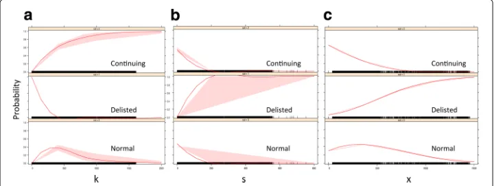
To investigate further, we performed an analysis of deviance to test the explanatory strength of interactive predictors. As shown in Table7, node degree, average neighbour degree, and strength were the first three influential terms that contributed the most to the reduction of residual deviance, i.e., 10919.2 fromki, 2979.8 fromxi, and 2777.2 from
si. This indicated that these three degree-based measures contributed more in terms
of reducing deviance to the resilient response probability when compared with other centrality measures.
Figure5 shows the effect displays of these three degree-based variables in terms of quantified probability for all three groups. In subplot (a) to (c), we can see the probability of being modelled as Delisted was relatively sensitive to the changes in these three vari-ables (probability value varies in full range from zero to one). In contrast, the sensitivity associated with Normal group fluctuated within a small range. For example, no matter how much drop or raise occurred in these three variables, the maximum probability of being modelled as Normal members were always less than 0.5. Meanwhile, their effects on modelling probability for Continuing group seemed to be in the middle of the former two.
Model testing
The multinomial logistics model was validated and tested using network data from the last five years of observation, 2012-2017. Taking 2012-2013 as an example, Fig.6depicts the Receiver Operating Characteristic (ROC) curve analysis of the model performance
Table 7Analysis of deviance
Variables Deviance Residual deviance
Intercept 122831
Intercept+k 10919 111912
Intercept+k+s 2777 109135
Intercept+k+s+k− 1520 107615
Intercept+k+s+k−+e 17 107598
Intercept+k+s+k−+e+c 737 106861
Fig. 5Effect displays analysis of the the three degree-based measures on all stock groups.adegree;bnode strength;caverage neighbour degree
when predicting the survivability resilience of the stocks during that time period. Because the ROC curve is normally used for binary classifiers, we plotted a one-vs-rest ROC curve for each class. The Area Under Curve (AUC) was adopted as an illustrative indica-tor that quantitatively demonstrated the diagnostic ability of the model. As shown in the figure, model performance with regard to predicting Delisted (AUC=0.733) and Contin-uing (AUC=0.702) stocks was relatively higher than when it was applied for predicting stocks from the Normal group (AUC=0.626). This might have resulted from the range of dynamic behaviour of network measures associated with stocks from different groups, which meant that the uniqueness of nodal interdependence from stocks in the Delisted and Continuing groups could potentially be more abnormal.
By observing ROC plots in Fig.7, it even further enhances such interpretation as the AUC values for the Delisted and Continuing groups remained relatively stable around 0.69 to 0.74, while the AUC for Normal group gradually decreased from 0.649 to 0.550, indi-cating an increasing difficulty to accurately identify stocks with normal nodal behaviour. However, that might have been more achievable if one considered the rationale behind the network measures of these interactive nodes. That is, the continuing stocks would very likely still exist in the near future and, because they were becoming more influential in the
Fig. 7ROC analysis of three groups of stocks ina2013-2014,b2014-2015,c2015-2016 andd2016-2017
core area of the market, then more stocks would tend to correlate with them. This would result in a growing interdependence degree within the networks. Of course, such growth would be heavily subjected to dynamic changes and shifts as the market evolved. However, stocks from the Normal group might also tend to waver between states of failure and con-tinuation, therefore making their accurate identification fairly difficult. Coincidentally, this matches with the sensitivity insights we found in the aforementioned effect display tests.
Fig. 9Distribution of the six network measures in 2016-2017.aDegree;bStength;cNegative degree;d Eigenvector;eCC;fAve. Neigh. degree
Conclusion
We addressed the issue of characterising a stock’s survivability resilience in terms of bankruptcy prediction, using interdependent correlation-based networks. Relying upon big financial market data, we constructed these weighted, signed, and temporal net-works based on correlations between stock pairs according to their daily adjusted closing prices. As a first step in exploring the dynamically evolving topology of the networks, we identified six suitable measures of network centrality and characterised different stock behaviours in terms of survivability. To maintain model transparency for each variable, we used those centrality measures as predictor variables in a weighted multinomial logistics model and conducted the further statistical analysis.
This study produced three main findings: First, the market, counterintuitively, does not constantly expand exponentially if one considers yearly dynamic “fission-fusion” shifting. Instead, major fluctuations occur, possibly because the market responds to unexpected external stimuli by dynamically adjusting nodal interdependence. Second, centrality-based network measures were useful predictive variables when characterising failed or resilient stocks because those measures can effectively capture the abnormal behaviour of such stocks. Finally, the results of analysis and model testing suggested that degree-based measures, including node degree, average neighbour degree, and node strength, could be applied as descriptive parameters for characterising the survivability resilience of equities in the London Stock Exchange. However, the effect of variables and AUC values obtained from the Normal group indicated that stocks from this group were more difficult to depict.
for identifying early signals of firms in potential financial difficulties, which can help for various decision- and policy-makers such as investors, creditors, and managers.
Appendix 1: Partial correlation coefficients with excess return
Taking 2016-2017 as an example, we constructed the network with Partial correlation coefficient method. The benchmark for calculating excess return was SPDR S&P 500 ETF index, which collected with a same periodicity within 2016-2017. The correlation matrix was obtained by applying Partial correlation coefficient function in MATLAB (Mathworks) with the residuals against the benchmark. The percentage of the positive coefficient was around 62.26% (dropping from 78.63% from Table3) with negative ones around 37.74%. This shows an interesting comparative result as the portion of negative correlations greatly increased.
Appendix 2: Distributions of six network measures in 2003-2004 and 2016-2017 Figures 8 and 9 illustrate the distribution of all six network measures with respect to dif-ferent groups of companies in 2003-2004 and 2016-2017. The aforementioned gaps were still obvious in those two later years. Because these differences in distribution remained throughout the observation period, one might infer that they were a general feature associated with each group rather than being simply random outcomes.
Abbreviations
AUC: Area under curve; CC: Clustering coefficient; ROC: Receiver operating characteristic
Acknowledgements
The research was conducted at the Future Resilient Systems at the Singapore-ETH Centre, which was established collaboratively between ETH Zurich and Singapore’s National Research Foundation (FI 370074011) under its Campus for Research Excellence and Technological Enterprise programme. All authors contributed to the conception and design of the study, have read and approved the final manuscript. The authors declare no conflict of interest and would like to thank Dr. Aakil M. Caunhye for his coordination in data collection.
Funding
This work is supported by ETH Zurich and Singapore’s National Research Foundation (Grant Number FI 370074011).
Availability of data and materials
Data are available upon request.
Authors’ contributions
Conceptualisation: JT, HRH, LK. Data curation: LK, JT. Formal analysis: JT, HRH, LK. Methodology: JT, HRH. Software: JT. Supervision: HRH, LK. Visualisation: JT. Original draft: JT, LK. Review & editing: JT, LK, HRH. All authors read and approved the final manuscript.
Competing interests
The authors declare that they have no competing interests.
Publisher’s Note
Springer Nature remains neutral with regard to jurisdictional claims in published maps and institutional affiliations.
Received: 15 February 2018 Accepted: 16 July 2018
References
Alaka HA, Oyedele LO, Owolabi HA, Kumar V, Ajayi SO, Akinade OO, Bilal M (2017) Systematic review of bankruptcy prediction models: Towards a framework for tool selection. Expert Syst Appl.https://doi.org/10.1016/j.eswa.2017.10.040 Allen F, Babus A (2009) Networks in finance. Wharton School Publishing Upper Saddle River, New Jersey
Altman E (1968) Financial ratios, discriminant analysis and the prediction of corporate bankruptcy. J Financ 23(4):589–609.https://doi.org/10.2307/2978933
Amendola A, Giordano F, Parrella ML, Restaino M (2017) Variable selection in high-dimensional regression: a
Anchuri P, Magdon-Ismail M (2012) Communities and balance in signed networks: A spectral approach. In: Proceedings of the 2012 International Conference on Advances in Social Networks Analysis and Mining (ASONAM 2012). IEEE Computer Society, Kadir Has University, Istanbul. pp 235–242.https://doi.org/10.1109/asonam.2012.48
Baba K, Sibuya M (2005) Equivalence of partial and conditional correlation coefficients. J Jpn Stat Soc 35(1):1–19.https:// doi.org/10.14490/jjss.35.1
Barabási A-L (2016) Network Science. Cambridge university press, Cambridge
Barboza F, Kimura H, Altman E (2017) Machine learning models and bankruptcy prediction. Expert Syst Appl 83:405–417. https://doi.org/10.1016/j.eswa.2017.04.006
Barrat A, Barthelemy M, Vespignani A (2008) Dynamical Processes on Complex Networks. Cambridge university press, Cambridge
Beaver WH (1966) Financial ratios as predictors of failure. J Account Res:71–111.https://doi.org/10.2307/2490171 Benesty J, Chen J, Huang Y, Cohen I (2009) Pearson correlation coefficient. In: Noise Reduction in Speech Processing.
Springer, Heidelberg. pp 1–4.https://doi.org/10.1007/978-3-642-00296-05
Bonacich P (1987) Power and centrality: A family of measures. Am J Sociol 92(5):1170–1182.https://doi.org/10.1086/ 228631
Bonanno G, Caldarelli G, Lillo F, Mantegna RN (2003) Topology of correlation-based minimal spanning trees in real and model markets. Phys Rev E 68(4):046130.https://doi.org/10.1103/physreve.68.046130
Bonanno G, Caldarelli G, Lillo F, Micciche S, Vandewalle N, Mantegna RN (2004) Networks of equities in financial markets. Eur Phys J B-Condens Matter Complex Syst 38(2):363–371.https://doi.org/10.1140/epjb/e2004-00129-6
Chawla NV, Bowyer KW, Hall LO, Kegelmeyer WP (2002) Smote: synthetic minority over-sampling technique. J Artif Intell Res 16:321–357.https://doi.org/10.1613/jair.953
Chi KT, Liu J, Lau FC (2010) A network perspective of the stock market. J Empir Financ 17(4):659–667.https://doi.org/10. 1016/j.jempfin.2010.04.008
Chiang K-Y, Hsieh C-J, Natarajan N, Dhillon IS, Tewari A (2014) Prediction and clustering in signed networks: a local to global perspective. J Mach Learn Res 15(1):1177–1213
Chong E, Han C, Park FC (2017) Deep learning networks for stock market analysis and prediction: Methodology, data representations, and case studies. Expert Syst Appl 83:187–205.https://doi.org/10.1016/j.eswa.2017.04.030 du Jardin P, Veganzones D, Séverin E (2017) Forecasting corporate bankruptcy using accrualbased models. Comput
Econ:1–37.https://doi.org/10.1007/s10614-017-9681-9
Erciyes K (2014) Complex Networks: an Algorithmic Perspective. CRC Press, Florida
Fruchterman TM, Reingold EM (1991) Graph drawing by force-directed placement. Softw Pract Experience 21(11):1129–1164.https://doi.org/10.1002/spe.4380211102
Gao Y-C, Wei Z-W, Wang B-H (2013) Dynamic evolution of financial network and its relation to economic crises. Int J Mod Phys C 24(02):1350005.https://doi.org/10.1142/s0129183113500058
Han J, Pei J, Kamber M (2011) Data Mining: Concepts and Techniques. Elsevier, Waltham
Heiberger RH (2014) Stock network stability in times of crisis. Physica A Stat Mech Appl 393:376–381.https://doi.org/10. 1016/j.physa.2013.08.053
Huang W-Q, Zhuang X-T, Yao S (2009) A network analysis of the chinese stock market. Physica A Stat Mech Appl 388(14):2956–2964.https://doi.org/10.1016/j.physa.2009.03.028
Jones S, Johnstone D, Wilson R (2017) Predicting corporate bankruptcy: An evaluation of alternative statistical frameworks. J Bus Finan Account 44(1-2):3–34.https://doi.org/10.1111/jbfa.12218
Kauê Dal’Maso Peron T, da Fontoura Costa L, Rodrigues FA (2012) The structure and resilience of financial market networks. Chaos Interdiscip J Nonlinear Sci 22(1):013117.https://doi.org/10.1063/1.3683467
Kenett DY, Tumminello M, Madi A, Gur-Gershgoren G, Mantegna RN, Ben-Jacob E (2010) Dominating clasp of the financial sector revealed by partial correlation analysis of the stock market. PLoS ONE 5(12):15032.https://doi.org/10. 1371/journal.pone.0015032
Khoja L, Chipulu M, Jayasekera R (2016) Analysing corporate insolvency in the gulf cooperation council using logistic regression and multidimensional scaling. Rev Quant Finan Acc 46(3):483–518. https://doi.org/10.1007/s11156-014-0476-y
Kuo RJ, Chen C, Hwang Y (2001) An intelligent stock trading decision support system through integration of genetic algorithm based fuzzy neural network and artificial neural network. Fuzzy Sets Syst 118(1):21–45.https://doi.org/10. 1016/s0165-0114(98)00399-6
Kwapie ´n J, O´swiecimka P, Forczek M, Dro˙zd˙z S (2017) Minimum spanning tree filtering of correlations for varying time scales and size of fluctuations. Phys Rev E 95(5):052313.https://doi.org/10.1103/physreve.95.052313
Lee KC, Han I, Kwon Y (1996) Hybrid neural network models for bankruptcy predictions. Decis Support Syst 18(1):63–72. https://doi.org/10.1016/0167-9236(96)00018-8
Leskovec J, Huttenlocher D, Kleinberg J (2010) Signed networks in social media. In: Proceedings of the SIGCHI Conference on Human Factors in Computing Systems. ACM, USA. pp 1361–1370.https://doi.org/10.1145/1753326.1753532 Ma Y, Zhang X-D (2018) Estimating the number of weak balance structures in signed networks. Commun Nonlinear Sci
Numer Simul 62:250–263.https://doi.org/10.1016/j.cnsns.2018.02.034
Mantegna RN (1999) Hierarchical structure in financial markets. Eur Phys J B-Condens Matter Complex Syst 11(1):193–197. https://doi.org/10.1007/s100510050929
Mathworks Linear or Rank Partial Correlation Coefficients.https://www.mathworks.com/help/stats/partialcorr.html. Accessed 14 May 2018
Montgomery DC, Peck EA, Vining GG (2012) Introduction to Linear Regression Analysis vol. 821. Wiley, New Jersey Mosley L (2013) A balanced approach to the multi-class imbalance problem. Doctor of Philosophy Thesis, Iowa State
University of Science and Technology, USA
Mossman CE, Bell GG, Swartz LM, Turtle H (1998) An empirical comparison of bankruptcy models. Financ Rev 33(2):35–54. https://doi.org/10.1111/j.1540-6288.1998.tb01367.x
Newman M (2010) Networks: an Introduction. Oxford university press, Oxford
Onnela J-P, Chakraborti A, Kaski K, Kertesz J, Kanto A (2003) Dynamics of market correlations: Taxonomy and portfolio analysis. Phys Rev E 68(5):056110.https://doi.org/10.1103/physreve.68.056110
Pour EK, Lasfer M (2013) Why do companies delist voluntarily from the stock market? J Bank Financ 37(12):4850–4860. https://doi.org/10.1016/j.jbankfin.2013.08.022
Rhim A (1993) Reorganization schemes under uk insolvency act of 1986: Chapter 11 as a springboard for discussion. Loy LA Int’l Comp LJ 16:985
Shumway T (2001) Forecasting bankruptcy more accurately: A simple hazard model. J Bus 74(1):101–124.https://doi.org/ 10.1086/209665
Singpurwalla ND (1995) Survival in dynamic environments. Stat Sci:86–103.https://doi.org/10.1002/9780470060346.ch7 Sterbenz JP, Hutchison D, Çetinkaya EK, Jabbar A, Rohrer JP, Schöller M, Smith P (2010) Resilience and survivability in
communication networks: Strategies, principles, and survey of disciplines. Comput Netw 54(8):1245–1265.https:// doi.org/10.1016/j.comnet.2010.03.005
Tang J, Khoja L, Heinimann HR (2017) Modeling stock survivability resilience in signed temporal networks: A study from london stock exchange. In: International Workshop on Complex Networks and Their Applications. Springer, France. pp 1041–1052
Ticknor JL (2013) A bayesian regularized artificial neural network for stock market forecasting. Expert Syst Appl 40(14):5501–5506.https://doi.org/10.1016/j.eswa.2013.04.013
Tumminello M, Aste T, Di Matteo T, Mantegna RN (2005) A tool for filtering information in complex systems. Proc Natl Acad Sci USA 102(30):10421–10426.https://doi.org/10.1073/pnas.0500298102
Vandewalle N, Brisbois F, Tordoir X (2001) Non-random topology of stock markets. Quant Finan 1(3):372–374.https://doi. org/10.1088/1469-7688/1/3/308
Xu R, Wong W-K, Chen G, Huang S (2017) Topological characteristics of the hong kong stock market: A test-based p-threshold approach to understanding network complexity. Sci Rep 7.https://doi.org/10.1038/srep41379 Xuan X, Murphy K (2007) Modeling changing dependency structure in multivariate time series. In: Proceedings of the 24th
International Conference on Machine Learning. ACM, USA. pp 1055–1062.https://doi.org/10.1145/1273496.1273629 Yook S-H, Jeong H, Barabási A-L, Tu Y (2001) Weighted evolving networks. Phys Rev Lett 86(25):5835.https://doi.org/10.
1103/physrevlett.86.5835
Zelenkov Y, Fedorova E, Chekrizov D (2017) Two-step classification method based on genetic algorithm for bankruptcy forecasting. Expert Syst Appl 88:393–401.https://doi.org/10.1016/j.eswa.2017.07.025
Zhang G, Hu MY, Patuwo BE, Indro DC (1999) Artificial neural networks in bankruptcy prediction: General framework and cross-validation analysis. Eur J Oper Res 116(1):16–32.https://doi.org/10.1016/s0377-2217(98)00051-4