Simulation of Visual Servo Control with Kalman Filter on Puma 560

Simulation of Visual Servo Control with Kalman

Filter on Puma 560

Noor Cholis Basjaruddin

Department of Electrical Engineering, Politeknik Negeri Bandung

Jl. Gegerkalong Hilir, Ds.Ciwaruga Kotak Pos 1234 Bandung Indonesia 40012, Phone: +62-22-2013789 [email protected]

Abstract— Pose estimation is important step on Position-Based Visual Servo Control System building. This paper presents a vision based position sensor system which provide three dimensional (3D) relative position and orientation (pose) of an arbitary moving object with respect to end-effector mounted camera. Kalman filtering is applied to vision measurement from a single end-effector mounted camera to implement an implicit real-time solution of the photogrametic equations and to provide significant temporal filtering of the resulting motion parameters. PUMA 560 robot is selected to implement this simulation. The kinematic and dynamic data of PUMA 560 is collected from references. Simulation is build with Matlab and Robotic Toolbox. Results of computer simulation demonstrate the successful operation of the control strategy and Kalman filter success to estimate relative pose.

Index Term-- visual servo control system; position-based visual control system; Kalman Filter; pose estimation

I. INTRODUCTION

Development of visual sensors for a robot getting closer to the ideal robot eye. This was especially true after the invention of computer vision technology that allows for image processing. Image processing technology in addition to allowing the camera to recognize a pattern (pattern recognition) is also able to recognize features (feature recognition).

Feature recognition technology allows the robot can carry out various activities such as walking into a place without having to remember all of what is seen during the trip. It is very important, especially related to limitations of data storage device and image data processing speed. Based on the ability to recognize a feature, robot eye is also capable of sensing an object with a good position relative to itself. This capability allows the robot - with cameras mounted on him - can grasp an object is moving towards. This visual based robot control system is called as visual servo control.

In this research, we build a visual servo control simulation of a PUMA 560 robot.The simulation results using dynamic model will be compared with simulation results without dynamic model. The Kalman filter is used in this system as pose estimator.

II. RESEARCH METHOD

A. Visual Servo Control

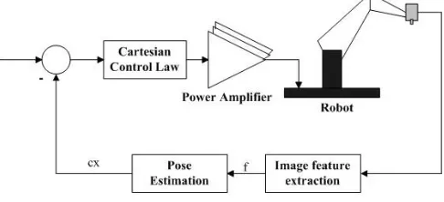
Position-based visual control system is used in this simulation. Block diagram of this system can be seen in Figure 1[8]_.

Fig. 1. Position-based visual control system

In this system, features are extracted from the images and used in conjunction with a geometric model of the target to determine the pose of the target with respect to the camera.

B. Kinematic Model

Kinematic model of PUMA 560 was built using Denavit Hartenberg (DH) transformation matrix representation. A schematic of the robot and the axis conventions used in shown in Figure 2. The kinematic constants for PUMA 560 are given in Table I.

Table I

Kinematic Parameters and joint limits for PUMA 560. All angels in degrees, lengths in mm

Joint αk ak dk min max

0 90 0 0 -180 180

1 0 431

,8

0 -170 165

2 -90 20,

3

150 -160 150

3 90 0 431,8 -180 180

5 -90 0 0 -10 100

Fig. 2. Detailed of coordinate frames used for the PUMA 560

C. Dynamic Model

Dynamic model was built based on Recursive Newton Euler's Equation (RNE). Each link has ten independent inertial parameters:

 Link mass, mi;

 Three first moments, which may be expressed as the COM location, si;

 Six second moments, which represent the inertia of the link about a given axis, typically through the COM. The second moments may be expressed in matrix form as

   

 

   

  

J J J

J J J

J J J

zz yz xz

yz yy xy

xz xy xx

J (1)

A 6-axis manipulator dynamic model thus entails 60 inertial parameters[8]_.

Table II Link Mass data (kg)

Parameter Value

m1 13,0

m2 17,4

m3 4,80

m4 0,82

m5 0,35

m6 0,09

Table III

Link COM position with respect to link frame (mm)

Parameter Value

sx1 -

sy1 -

sz1 -

sx2 -363,8

sy2 6

sz2 77,4

sx3 0

sy3 -14

sz3 70

sx4 0

sy4 -19

sz4 0

sx5 0

sy5 0

sz5 0

sx6 0

sy6 0

sz6 32

Table IV

Link Inertia about the COM (kg.m2₎ Parameter Value

Jxx1 -

Jyy1 0,35

Jzz1 -

Jxx2 0,130

Jyy2 0,524

Jzz2 0,539

Jxx3 0,066

Jyy3 0,0125

Jzz3 0,086

Jxx4 1,8e-3

Jyy4 1,8e-3

Jzz4 1,3e-3

Jxx5 0,30e-3

Jyy5 0,30e-3

Jzz5 0,40e-3

Jxx6 0,15e-3

Jyy6 0,15e-3

Jzz6 0,04e-3

D. Kinematics of camera mount and lens

This section analyses two important mapping in visual servo system. The first is the mapping between robot wrist motion and motion of the camera which is a function of kinematics of the camera mounting on the end-effector. The second is the mapping between camera motion or target motion and perceived motion on the image plane. Mass and inertia of camera are given in Table V.

Camera mount kinematics

To simplify analysis it is desirable to mount the camera such that camera DOF are controlled individually by robot wrist axes. Jacobian matrix at wrist or T6 is[12],

   

   

J J

0 J ) ( J

22 21 11 θ

t6

(2)

J22 describes and-effector rotation due to wrist axis and

motion, and J21 describes rotation of the end-effector due to

base axis motion which is assumed zero in this case. Camera mount used in this research is shown in Figure 3.

Table V Mass and Inertia of camera

Parameter Value

mlens 0,270 kg

mcamera 0,155 kg

lzz 1,0 x 10-3

kgm2

lxx 6,2 x 10-3

kgm2

l1 0,417

kgm2

 0,034

 0,005

Fig. 3. Camera mount used in this research

The camera mounting arrangement shown in Figure 3 can be seen intuitively to couple camera pan and tilt motion to wrist axes 6 and 5 respectively.

 

 

 J J ( )

x c _t66 _θ

c (3)                            pan tilt 6 5 1 0 0 S6 1 -    (4)

Camera roll rate is shown as

roll= - C6₅ (5)

E. 3D Pose Estimation Using the Extended Kalman Filter The first step in the relative pose estimation is the establishment of the geometric relationship between feature points defined in an object frame and the corresponding image plane points in the camera frame[13]_.

Geometric Relationships

Fig. 4. Object Feature Image Projection

The geometrics of the problem is illustrated in Figure 4 and the nomenclature used is as follows:

Oo _{- X}o_Yo_Zo _{Object reference frame,}

Oc _{- X}c_Yc_Zc _{Camera refence frame with Z}c _{– axis}

coinciding with the optical axis,

Oi _{– X}i_Yi _{Image reference frame,}

F Camera focal length,

T o j o j o j o

j (X ,Y ,Z )

P  Coordinate vector of the jth object feature point in the object frame

T c j c j c j c

j (X ,Y,Z )

P  Coordinate vector of the _{point in the camera frame} jth object feature

i j i j,y

x Corresponding projection of the jth feature point coodinates in the image frame,

Px, Py Inter-pixel spacing along the xi _{and y}i _axes

(m/pixel),





Z Y, X,

T Relative position vector, ϕ,α,ψ Relative roll, pitch, dan yaw

o

j c

j

T

R(

,

α,

ψ)

P

P







Where

P

and R(ϕ,α,ψ) is the rotation matrix

R(ϕ,α,ψ)=                                         C C S C S C C C S S C C S S S C S S S S S C C S S S C C C ψ ψ ψ ψ ψ ψ (7)

For the point projection camera model shown in Figure 4, the corresponding projection feature point locations in the image frame are obtained by

c j y c j i j c j x c j i j Z P FY y , Z P FX

x   (8)

Combaining Eq.(6) and Eq.(8) results in the equations defining the image feature locations as nonlinier functions of the pose parameters and the known feature point coordinates in the object frame.

Kalman Filter Algorithm

The Kalman filters defines the optimal estimate of the states with dynamics specified through a linear state space dynamical model and the output measurements defined as a linear function of the states. It also assumes that zero mean Gaussian noise characterizes disturbance inputs to the dynamic model and output measurement errors.

model, T is the sample period, and k is the sample time. The discrete time dynamical system model is then

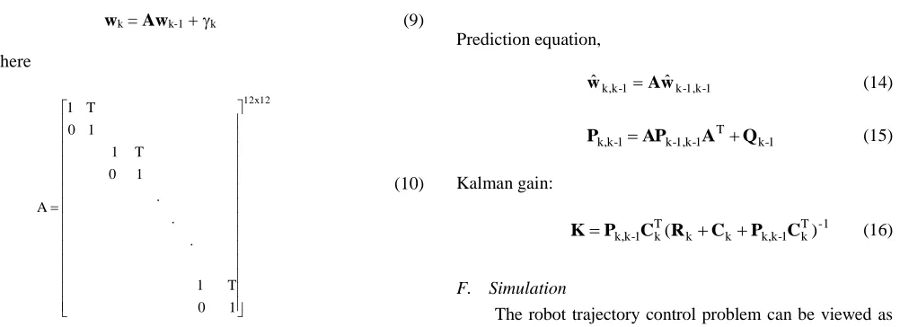
wk = Awk-1 + k (9)

where 12 x 12 1 0 T 1 . . . 1 0 T 1 1 0 T 1 A                                  (10)

The Kalman output model is then obtained from Eq.6 and Eq.8 as

zk = G(wk) + vk (11)

where





k i 3 i 3 i 2 i 2 i 1 i

1,y ,x ,y ,x ,y

x k 

z (12)

         c 3 y c 3 c 3 x c 3 c 2 y c 2 c 2 x c 2 c 1 y c 1 c 1 x c 1 Z P Y , Z P X , Z P Y , Z P X , Z P Y , Z P X F -k) (w G (13)

vk is measurement noise which is assumed to be described by zero mean Gaussian noise with covariance R.

The recursive equations defining the extended Kalman filter algorithm are given by the following:

Prediction equation, 1 -k 1, -k 1 -k k, ˆ

ˆ Aw

w  (14)

1 -k T 1 -k 1, -k 1 -k

k, AP A Q

P   (15)

Kalman gain: -1 T k 1 -k k, k k T k 1 -k

k, C (R C P C )

P

K   (16)

F. Simulation

The robot trajectory control problem can be viewed as the control of the end-point with respect to a coordinate frame attached to the object as shown in Figure 5. Block diagram of system is shown in Figure 6.

Base Object B O W B E W O E W O Ereff W E E W 

Fig. 5. System Vector Relationships

III. RESULTS AND ANALYSIS

A. Pose Estimation Simulation Results

Figure 7 shows one of simulation results with the matrix R is a diagonal matrix with diagonal elements 1000 and the matrix Q is also a diagonal matrix with diagonal elements 0.01.

Fig. 7. Pose Estimation with Kalman Filter

This simulation gives the conclusion that the greater value of the matrix elements of R will make the Kalman filter is more accurate in pose estimating of the robot in the direction of X and Y.

B. Closed Loop System Simulation Results

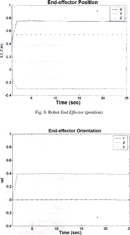
In this simulation PUMA 560 desired reach the pose as given by the matrix (W_Erefo ). Initial position of the robot is set at zero pose (Xip).

o Eref

W =

       

 

       

  

0 3927 , 0

0 5376 , 0

300 , 0 7574 , 0

Xip =

       

 

       

  

0 0 0 4318 , 0

150 , 0 4521 , 0

Simulation results are shown in Figure 8 and Figure 9.

Orientation

Fig. 8. Robot End Effector (position)

Fig. 9. Robot End Effector (orientation)

The simulation results show that the robot can reach the position and orientation in accordance with set point

(W_Erefo ). Error average in this simulation is below 5%.

C. Trajectories Tracking Simulation Results

Figure 10 and Figure 11 show results of trajectories tracking simulation.

Fig. 10. Trajectory Tracking (position)

Fig. 11. Trajectory Tracking (orientation)

In general, the system can follow a given trajectory (Xsp,Ysp,Zsp,rsp,psp,ysp). The biggest error is when the system

is following the roll angle trajectory (rsp). Ability in tracking

highly influenced by the selection of matrix Q and R as well as tuning of PID.

IV. CONCLUSION

Simulations using the dynamic model showed better results than the simulations that only use the kinematic model. Election Q and R matrices in Kalman filter will affect the accuracy of the robot pose estimation. In addition, the selection of matrix Q and R are not exactly going to make the simulation process becomes divergent and not

successfully implemented. Extended Kalman Filter can be used as an robot pose estimator and can be used in visual servo control system

REFERENCES

[1] J.Hill and WT Park, “Real Time Control of a Robot with a Mobile Camera, 9th_{”, International Symposium on Industrial Robots, March}

1979; pp-233-246.

[2] J.Wang, WJ.Wilson, “3D Relative Position and Orientation Estimation Using Kalman Filtering for Robust Control”, Proceedings for the 1992 IEEE Robotics and Automation Conference, Nice, France, May 10-15, 1992

[3] KS.Fu et.al, “Robotics, Control, Sensing, Vision and Intelligence”, McGrawHill International Editions, Singapura, 1987

[4] Koichi Hashimoto, “Visual Servoing Real Time Control of Robot Manipulator Based on Visual Sensory Feedback”, World Scientific Publishing, Singapura, 1993

[5] Luh, J.Y.S et.al, “On-Line Computational Scheme for Mechanical Manipulators", Trans.ASME, J.Dynamic Systems, Measurements and Control, vol.120, pp.69-76

[6] Noor Cholis Basjaruddin, “Simulasi Kendali Servo Visual Dengan Tapis Kalman Sebagai Estimator Sikap Pada Robot PUMA 560”, Tesis, Program Pascasarjana ITB, Bandung, 2002

[7] PI. Corke, “Visual Control of Robot Manipulators - A Review”, CSIRO, Australia, 1993

[8] PI.Corke, “Visual Control of Robots, High-Performance Visual Servoing”, John Wiley & Sons Inc, New York, 1996

[9] PI. Corke, “Robotic Toolbox (release 5)”,Pinjarra Hills, Australia, 1999

[10] RD Klafter, TA. Chmielewski, and M.Negin, “Robotic Engineering An Integrated Approach”, Prentice Hall, USA, 1989

[11] Robert Grover Brown & Patrick YC Hwang, “Introduction to Random Signals and Applied Kalman Filtering”, John Wiley & Sons Inc, Canada, 1997

[12] R.P.Paul and H.Zhang, ”Computationally efficient kinematics for manipulators with spherical wrists base”, International Journal of Robotics Research, Volume 5 Issue 2, Summer, CA, USA,1986 [13] William J Wilson, “Visual Servo Control of Robots Using Kalman