COMPARATIVE ANALYSIS OF THE GREEDY METHOD AND DYNAMIC PROGRAMMING IN SOLVING THE KNAPSACK PROBLEM.

(1)

http://www.gjaets.com © Global Journal of Advance Engineering Technology and Sciences 62

Global Journal of Advanced Engineering Technologies and Sciences

COMPARATIVE ANALYSIS OF THE GREEDY METHOD AND

DYNAMIC PROGRAMMING IN SOLVING THE KNAPSACK PROBLEM

Oluyinka I. Omotosho

*1

, Aderemi E. Okeyinka

2

*1_{Department of Computer Science and Engineering, Ladoke Akintola University of Technology,}

PMB 4000, Ogbomosho, Oyo state, Nigeria.

2_{School of Physical Sciences, Landmark University, Omu-aran, Kwara state, Nigeria.}

Abstract

In this work, two of the existing algorithms for solving the Knapsack are investigated and implemented using the same programming language. The complexity of the programs and hence the algorithms were measured to determine the more efficient of the two algorithm. The result of this comparative study of complexity is that Greedy algorithm is more efficient for solving knapsack problem than dynamic programming approach.

Keywords:Greedy algorithm, Dynamic Programming, Comlexity, Knapsack model.

Introduction

The success of a practical management of any organisation, including the conduct and co-ordination of the operations or activities within the organisation, be it business, industries, governmental agencies hospital and so forth, highly depends on the ability to provide, understandable conclusions to the decision maker(s), when they are needed. Rather than being content with merely improving the status quo, the goal is to identify the best or optimal solution to the problem under consideration [1]. The real life applications, such as assignment of personnel, blending of materials, distribution and transportation of goods/sales effort, production planning, budget allocation and so forth are highly characterised by the need to allocate limited resources among various items involved [2].This is a special resource allocation problem that is concerned with the task of filling the knapsack (a container) from the possible maximum selected weight say Wj that maximizes the total profit that can be earned from the selected weights to fill the knapsack almost exactly. This implies that at most the accumulated weight must not exceed M, knapsack capacity. Any class of problems in network optimisation, be it transportation, communication, production planning and so forth, with a resemblance of the above is a knapsack problem [3].Two versions of the knapsack problem are 0-1 and fractional knapsack problem [10]. This paper employs the Greedy Method, [4] and Dynamic Programming method, [5]. Both techniques are solution strategies for solving the knapsack and the related problems. This paper analyses and compares the performance of the various algorithms based on these two techniques for solving the knapsack problem, from the points of view of program complexity, optimal values and values of the constraint functions.

Related Works

A greedy algorithm for optimization problem always make the choice that looks best at the moment and adds is it to best solution[9]. Greedy algorithms don’t always yield optimal solutions but, when they do, they are usually the simplest and most efficient algorithm [9]. Most of the problems solvable by the Greedy method have n inputs and requires one to obtain a subset that satisfies some constraints [1]. The dynamic programming method can be used when the solution to a problem may be viewed as a result of sequence of decisions [5].

It is used when the solution can be recursively described in terms of solutions to subproblems [10] Dynamic programming algorithms finds solution to subproblems and stores them in memory for later use [10]. Horozitz and Sahni [6] extended the dynamic programming approach to include a divide and conquer scheme and showed that the problem can be solved in time 0(2n/2_{). Denardo [8] considered the 0/1 knapsack problem as a special case of resource}

(2)

tendency has a large payoff in computing where time means money and efficiency saves dollars [6]. For any algorithm the choice of test input depends on the complexity of the program though with some other factors [8]. This paper work is a comparative study of two optimization techniques, Dynamic Programming and Greedy method, of solving the knapsack problem.

METHODS

This methods considered in this paper are Greedy Method and Dynamic programming method, as solution strategies in solving the knapsack problem. Each are explained in subsequent sections.

The greedy method

The greedy method works in stages, considering one input at a time. At each stage, a decision is made whether the inclusion of a particular input will result in an optimal solution. This is done by considering the inputs in an order that is determined by some selection procedure. If the inclusion of the next input into a partially constructed optimal solution will result in an infeasible solution , then this input is discarded. The input selection procedure itself is based on some optimisation measure. This measure may or may not be the objective function. Therefore Greedy method provides a set of feasible solutions from which the optimal solution is selected.

Objective function: the quantity to be optimized i.e. maximizes or minimizes as the case may be.

Feasible Solution: a subset of inputs that satisfy the given constraints around the objective function that is, solution within the feasible region.

Optimal Solution: a feasible solution that either maximizes or minimizes the objective function. Given a knapsack problem formally stated as :

∑ 𝑃𝑖𝑋𝑖

1≤𝑖≤𝑛

∑ 𝑊𝑖𝑋𝑖

1≤𝑖≤𝑛

and 0 < Xi < 1, Pi > 0, Wi > 0, 1 < i < n, (3)

A feasible solution or filling is any set (Xi, X2,...Xn ), satisfying equations (2) and (3), while an optimal solution

is a feasible solution for which (1) is maximum.

A greedy algorithm suggests that at each step we include that object which has a maximum profit per unit of capacity used. When applying the greedy method to the solution of the knapsack problem there are at least three different measures one can attempt to optimise, when determining which object to include next [9]. These are the total profit or largest profit, the capacity used and the ratio of accumulated profit divided by the capacity used. If profit is used as the measure, then at each step we will choose an object an object that increases the profit most.

If the capacity measure is used , the next object included will increase this at least . Greedy based algorithms using the first two measures do not guarantee optimal solutions for the knapsack problem. Horowitz and sahni [7] have showm that a greedy algorithm using the third strategy always obtains an optimal solution . Therefore the object will be considered for inclusion in order of the ratio Pi/wi. The algorithms assume that the objects are sorted into non increasing order Pi/Wi. Algorithm for solving the knapsack problem is given in Algorithm 1.

Procedure Greedy-Knapsack (P, W, M, X, n)

(* P(l: n) and W( l:n) contain the profits and weights, respectively, of the n objects ordered so that P(i) P(i) > P(i +1) P(i +1) . M is the Knapsack size and X (1: n) is the solution vector *) real P( 1 :n), W (1: n), X(l :n), M, Cu;

integer i, n;

x <--- 0 (* initialise Solution to zero *)

≤

M

(2)

(1)

Maximize

(3)

Cu — M (* Cu = Remaining Knapsack capacity *) For 1 <--- 1 to n do

If W(i) > Cu then exit end if X(i) <--- 1

Cu <--- Cu – W end for

If I ≤ n then X(i) <--- Cu/W(i) end if End greedy – Knapsack

Algorithm 1: Greedy Algorithm for the Knapsack problem Weaknesses of Greedy Method

1. It does not give an overall optimal solution; it only gives an optimal solution for a particular unit at a point in time. This implies it only solves a problem statically.

2. The solution area of the Greedy strategy to the Knapsack problem is limited. In other words it cannot be applied to a large number of realistic cases.

Dynamic Programming method

Dynamic programming deals basically with optimization of multistage decision processes, where decisions are made sequentially at many points in time. It provides a method of avoiding the enumeration of all decision sequences in order to pick out the best [7]. It drastically reduces the amount of enumeration by avoiding the enumeration of some decision sequence that cannot possibly be optimal, i.e. Dynamic programming takes care of non-linarites, discontinuities, and local maximal or minimal to which linear programming cannot be successfully applied. In dynamic Programming, an optimal sequence of decisions is arrived at by making explicit appeal to the principle of optimality [8]. An optimal policy has the property that whatever the initial state and initial decisions, the remaining decisions must constitute an optimal policy with regard to the state resulting from the first decision ".

A Solution to the 0/1 knapsack problem is obtainable by making a sequence of decisions on the variables X1, X2

,...Xn. A decision on variable X; involves deciding which of the values 0 or 1 is to be assigned to it. In this case, the

sequential process breaks the problems involving several variables into a sequence of simpler problems each involving several variables into sequence of simpler problems each prior decision not affected by subsequent decisions. Each component problem can then be solved by the available procedure, usually the enumeration rechnique.

The essential characteristic of dynamic programming is a series of decisions distributed in time, where there is a interrelationship between decisions. Due to this interrelationship current decisions cannot be made independent of future decisions.

A return function which evaluates the choice made at each decision in terms of the contribution the decision can make to the overall objective (Minimized or maximized) is associated with each decision at every stage The total decision process at each stage is related to its adjoining stages by a quantitative, relationship called the transition function, which can reflect discrete or continuous quantities depending on the problem.

(4)

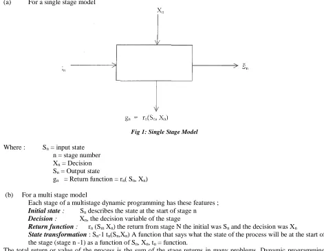
(a) For a single stage model

Fig 1: Single Stage Model

Where : Sn = input state

n = stage number Xn = Decision

Sn = Output state

gn = Return function = rn( Sn, Xn)

(b) For a multi stage model

Each stage of a multistage dynamic programming has these features ;

Initial state : Sn describes the state at the start of stage n Decision : Xn, the decision variable of the stage

Return function : rn (Sm Xn) the return from stage N the initial was Sn and the decision was Xn

State transformation : Sn-1 tn(Sn,Xn) A function that says what the state of the process will be at the start of

the stage (stage n -1) as a function of Sn, Xn, tn = function.

The total return or value of the process is the sum of the stage returns in many problems. Dynamic programming equations therefore, relates total optimal return with n stages to go. i.e, Fn(Sn) to the stage n return plus the value of

the remaining n - 1 stages [8]

Fn(Sn) = Opt { rn (Sn, Xn) + Fn_! (Sn-l)}

Subject to SN -i = tn( Sn ,Xn) = Sn - Xn

Therefore Dynamic programming is characterized by;

INPUT

Figure 2:

(5)

i. Stages: Point of decision making ii. States : input parameters

iii. Transformation : Equation or rule governing the decision iv. Decision

The Algorithm 2 gives the solution to the problem using this strategy [10]

Procedure Dynamic(P,W, stage, iternno,)

(* P(l, n) and W( 1: n) contain profit and weights respectively of the n objects without any specific order *) realP(l: n), W(l:n), x(l:n), stage,S(l:n, l:m)

integer i, n, a, b, c, d for i <--- 1 to n do

for stage <---1 to stage<-itemno xi --- 0

for i ---- 1 to n if xi <--- 0 c[stage]+I --- 0 else

c[ stage]+1  b[stage]*xi; else

if xi  0 for I  I to n

a[stage]+I  (b[stage-l]+I xi  1

st  w * x;

for 1  1 to n

if a[stage + I > b[stage] +1 cfstage] + I  a[stage] +1; d[stage] +1  0

else

c[stage] +1  b[stage] +1; d[stage] +1  1 endif

endfor endfor

endfor

w  a[I] * c[I] tw  tw + w p  b[i]* c[i] tp  tp + p; endif

endif endif endfor

Algorithm 2: Dynamic Programming Algorithm for the Knapsack problem Benefits of Dynamic Programming method

1. Produces an optimal solution to realistic knapsack problems" with a very wide. Solution area contrary to the Greedy strategy.

2. It does have a long term solution.

Limitations of Dynamic Programming method

(6)

2. Every dynamic programming is distinct,there is no fixed rule or procedure to flow in formulating problem i.e. particular equations used must be developed to fit each individual situation.

1. Dynamic Programming is effective for problems with multistage sequential decisions, hence could not be applied to single stage problems where decisions are made at one point in time.

Comparative Measure For Both Technques

In this work, three criteria are considered to analyses the two techniques. These are; i. Program Complexity measure

ii. Objective function optimal values (£ PiXj) iii. Constraint function values

Program Complexity measure

The most formidable measure for comparing two algorithms still remains the complexity computation in computer science. In this work, the Halstead complexity metrics are used to measure the program complexity of both techniques based on their program segment (procedure)

4.1.1 Demonstration of Halstead complexity metric with the Greedy solution program Segment;

Void Greedy( )

{

Cu=mk;

For(i= l; I <=; ++1)

{if ( w[i] > Cu)

{

if((cu > 0 ) && (i <= n))

x[i] = cu/w[i]

else

x[i] = 0;

}

else

x[i] = l;

Cu = Cu – w[i];

SumP+ = X[i] * P[i];

SumW+ = X[i] * W[i];

}

From the above, the program volume of the Greedy solution segment is given by; V(F) = N log n, where N = 76

n = 33 V(F) = 76 log 33

= 115.41

n N

2 2

1 1

4 4

7 12

4 5

- 1

5 12

2 6

1 1

- 4

1 1

- 4

1 6

3 7

1 7

- 1

(7)

Demonstration of Halstead complexity metric with the Dynamic Programming solution program Segment

Void Dynamic() {

for(i=l;i,=n;++l) {

for(stage=1; stage<=itemno ;++stage) xi=0

for(i=stage;i<=n;++1) {

if (stage==l) {

if(xi==0){ *(c[stage]+i =0; }

else *(c[stage]+i=b[stage]*xi; }

else{ if(xi=0) {

for(i=0;<=n;++i) {

*(a[stage]+I = *(b[stage-l]+I); }

xi = 1 ; st = w * x; for(i=0;K=n;++l) {

if (*(a[stage + 1) > *(b[stage] + 1)) {

cfstage] + i=a[ stage] + 1; d[stage] + i=0

else {

c[stage] + i=(b[stage] + 1; d[stage] + i=l;

} }

w = a[I] * c[I]; tw = tw + w; p = b[i]*c[i]; tp = tp + p; }

Hence, the program volume of the Greedy solution Program segment is given by; V(F) = N log n , where N = 194

n= 37 V(F) = 1941og37

= 304.29

n N

2 2

1 1

7 12

3 3

3 12 - 1 5 12 - 11 - 1 - 5

1 1

- 6

1 4

3 9

1 1

- 2 - 5 - 1 12 - 1

1 9

- 1 - 4

2 6

- 12 - 1 - 11 - 1 - 8 - 1 - 1 - 7 - 6 - 1 - 1

2 6

1 6

(8)

Objective Function Optimal values and Constraint Function values

As part of the criteria to measure and compare the performance of the two design techniques as they are applied to the knapsack problem, the algorithms 1 and 2 are not only used to compute the programs complexity, but also to measure and compute the optimal value of the objective function and the value of the Constraint function.

Simulation Description

Nine randomly generated data sets, ranging from 10 to 175, were used for each program. The data set were chosen to be 10, 20, 30, 40, 75, 100,125, 150 and 175. For Set n, similar problem instances were randomly generated using a random number generator. Each data set satisfies the following; random Wi and Pi, Wi Z [1,100],

Pi S [1,100], M =

∑ 𝑊𝑖/2

𝑛

1

The following formulars are used to generate the profits and weights, respectively. Profit = trunk [ 100 x RAN + C]

Weight = trunk [100 x RAN + C], Where C is any constant and RAN is the Random number generating function.

The computation of the optimal value of the objective function, that is, the maximum profit, £PiXi, the value of the constant function, that is, the maximum capacity of knapsack filled, ZWiXi, and the solution vector (Decision variable) are as described in section three.

Result Analysis And Discussion

Programming Complexity measure

From the result of the program complexity computation, based on the Halstead metric in sections 4.1.1 and 4.1.2. respectively as shown in Table 2, it could be observed that the Greedy program version has a volume of 115.41 while dynamic programming version has a volume of 304.29. This implies that Dynamic Programming version is more complex and voluminous than does Greedy method.

Optimal value Computation

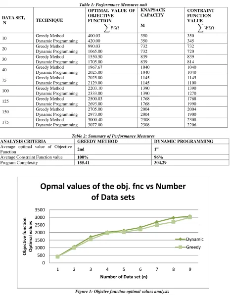
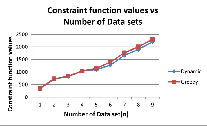
From the results or outputs of the program execution; as shown in table 2, it could be observed that by using the greedy method, the knapsack is being always filled to it's full capacity, since the value of the constant function ∑ 𝑊𝑖𝑋𝑖is always equal to the knapsack capacity, for all the data sets. However, this method gives the minimum profit, as the optimal value of the objective function ∑ 𝑃𝑖𝑋𝑖 is the lower for all the data sets . Figures 1 land 2 show these results , graphically.

The dynamic programming technique gives a better value of the objective function than the greedy method. It increases the optimal value of the objective function by an average of 6.27% of the greedy method. For n =1, the constraint function value is 99% of the knapsack capacity, 98% for n=125, 95% for n=150 and 96% for n=175, giving an average of 96%. Therefore the dynamic programming technique will on the average, fill 96% of the knapsack with a profit of 6.27% better than the greedy method. From the results the conclusion is that, based on the optimal value for the objective function, the dynamic programming technique is better than the greedy method for the solution to the 0/1 knapsack problem.

The results are clearly shown in the graphical representation of Figs 1 and 2. The averages, which are reported in this section, are computed directly from the tables. The percentage for the constant function values is computed by dividing the constant function by the capacity of the knapsack, and multiplying the result by 100, while the average is computed by dividing the sum of percentages by the number of groups of the sets, 9.

The performance of one method, x, over the, y, is computed by using the formula

(9)

Table 1: Performance Measures unit

DATA SET,

N TECHNIQUE

OPTIMAL VALUE OF OBJECTIVE FUNCTION ∑ 𝑃𝑖𝑋𝑖 KNAPSACK CAPACITY M CONTRAINT FUNCTION VALUE ∑ 𝑊𝑖𝑋𝑖

10 Greedy Method Dynamic Programming 400.03 420.00 350 350 350 345

Table 2: Summary of Performance Measures

ANALYSIS CRITERIA GREEDY METHOD DYNAMIC PROGRAMMING Average optimal value of Objective

Function 2nd 1

st

Average Constraint Function value 100% 96%

Program Complexity 155.41 304.29

Figure 1: Objctive function optimal values analysis

0 500 1000 1500 2000 2500 3000 3500

1 2 3 4 5 6 7 8 9

O b je ct iv e f u n ct ion O p ti m al v al u e s

Number of Data set (n)

Opmal values of the obj. fnc vs Number

of Data sets

(10)

Figure 2: Constraint function optimal values analysis

Conclusion

This paper has been able to analyse and compare two basic techniques; Greedy method and Dynamic programming, for solving the knapsack problem. Their performances are measured against the program complexity, optimal value of the objective function and value of the constraint function. Dynamic Programming has been considered to be effective and efficient than the Greedy method since it yields better optimal value of the objective function than does the Greedy. Also, dynamic programming yields an overall optimal solution over long period of time unlike the greedy method which only gives the optimal solution for particular stage or period. Though the Greedy method program is less complex to write, has less program volume and simpler to construct, than the Dynamic Programming, it is not as applicable for practical purposes as does dynamic programming.

References

1.

Wagner, H.M., (1989) "Principles of Operations Research, with Managerial Decisions", 2nd_{Edition, prentice}

Hall, Inc. Cliffs, N.J.

2.

Frederick, S. Hillier, and Gerald J. Lieberman, (1967,1975) "Operation Research". Second Edition, Holden-Day, Inc.

3.

Ingariola, G., and Korsh, J., "A general algorithm for one dimensional knapsack problems", Operation Research, 25(5), Ingargiola, G., and Korsh, J., (1973) "A reduction algorithm for zero-one single knapsack problems", Management Science, 20(4), pp.460-663.

4.

Magazine, m., Nemhauser, G., and Trotter, L., (1975) "When the Greedy solution solves aclass of knapsack problems", operation Research, 23(2).

5.

Nemhauser, G., and Ullman, Z., (1969) "Discrete dynamic programming and capital allocation", management science, 15(9).

6.

Horowitz, E., and Sahni, S., (1974) "Computing partitions with applications to the knapsack problem", J.ACM, 21(2), pp.277-292.

7.

Denardo, E.V, and Fox B.L, (1980) "Enforcing constraints on Expanded Networks".

8.

Denardo, E.V, (1982) "Dynamic Programming, models and Application Prentice-Hall, Inc. Englewood cliffs, New Jersey 07632, 2015.

9.

CLRS SECTION 16. Lecture 14: Greedy Algorithms, http://www.cse.ust.<k>-dekai.notes.

10.

Goddard S. Dynamic programming 0-1 Knapsack problem. http://www.cse.uni.edu/-goddard/Courses/CSCE310J, 20015.

0 500 1000 1500 2000 2500

1 2 3 4 5 6 7 8 9

COMPARATIVE ANALYSIS OF THE GREEDY METHOD AND DYNAMIC PROGRAMMING IN SOLVING THE KNAPSACK PROBLEM.

Global Journal of Advanced Engineering Technologies and Sciences