Machine Learning Reveals Missing Edges and Putative
Interaction Mechanisms in Microbial Ecosystem Networks
Demetrius DiMucci,
a,bMark Kon,
a,cDaniel Segrè
a,b,d,e,faBioinformatics Graduate Program, Boston University, Boston, Massachusetts, USA
bBiological Design Center, Boston University, Boston, Massachusetts, USA
cDepartment of Mathematics and Statistics, Boston University, Boston, Massachusetts, USA
dDepartment of Biology, Boston University, Boston, Massachusetts, USA
eDepartment of Biomedical Engineering, Boston University, Boston, Massachusetts, USA
fDepartment of Physics, Boston University, Boston, Massachusetts, USA
ABSTRACT
Microbes affect each other’s growth in multiple, often elusive, ways. The
ensuing interdependencies form complex networks, believed to reflect taxonomic
composition as well as community-level functional properties and dynamics. The
elucidation of these networks is often pursued by measuring pairwise interactions in
coculture experiments. However, the combinatorial complexity precludes an
exhaus-tive experimental analysis of pairwise interactions, even for moderately sized
micro-bial communities. Here, we used a machine learning random forest approach to
ad-dress this challenge. In particular, we show how partial knowledge of a microbial
interaction network, combined with trait-level representations of individual microbial
species, can provide accurate inference of missing edges in the network and
puta-tive mechanisms underlying the interactions. We applied our algorithm to three case
studies: an experimentally mapped network of interactions between auxotrophic
Escherichia coli
strains, a community of soil microbes, and a large
in silico
network of
metabolic interdependencies between 100 human gut-associated bacteria. For this
last case, 5% of the network was sufficient to predict the remaining 95% with 80%
accuracy, and the mechanistic hypotheses produced by the algorithm accurately
re-flected known metabolic exchanges. Our approach, broadly applicable to any
micro-bial or other ecological network, may drive the discovery of new interactions and
new molecular mechanisms, both for therapeutic interventions involving natural
communities and for the rational design of synthetic consortia.
IMPORTANCE
Different organisms in a microbial community may drastically affect
each other’s growth phenotypes, significantly affecting the community dynamics,
with important implications for human and environmental health. Novel culturing
methods and the decreasing costs of sequencing will gradually enable
high-throughput measurements of pairwise interactions in systematic coculturing studies.
However, a thorough characterization of all interactions that occur within a
micro-bial community is greatly limited both by the combinatorial complexity of possible
assortments and by the limited biological insight that interaction measurements
typ-ically provide without laborious specific follow-ups. Here, we show how a simple
and flexible formal representation of microbial pairs can be used for the
classifica-tion of interacclassifica-tions via machine learning. The approach we propose predicts with
high accuracy the outcome of yet-to-be performed experiments and generates
test-able hypotheses about the mechanisms of specific interactions.
KEYWORDS
coculture experiments, ecological networks, flux balance analysis,
machine learning, metabolic modeling, microbial interactions, microbiome, random
forests, synthetic ecology, systems biology
Received7 September 2018Accepted26
September 2018 Published30 October 2018
CitationDiMucci D, Kon M, Segrè D. 2018.
Machine learning reveals missing edges and putative interaction mechanisms in microbial ecosystem networks. mSystems 3:e00181-18. https://doi.org/10.1128/mSystems.00181-18.
EditorNassos Typas, Heidelberg University
Copyright© 2018 DiMucci et al. This is an
open-access article distributed under the terms of theCreative Commons Attribution 4.0 International license.
Address correspondence to Daniel Segrè, [email protected].
Ecological and Evolutionary Science
crossm
on September 8, 2020 by guest
http://msystems.asm.org/
lean and likely insurmountable task for even a moderately sized community. However,
it is conceivable that new computational approaches could systematically complement
existing tools such as high-throughput sequencing and genome annotation (14–18) to
help extract as much information as possible from interaction data sets, providing
insight both on yet-to-be-measured interactions and on the possible biological
mech-anisms mediating the specific partnerships.
Here, we present a conceptual framework for the mathematical representation of
microbial interactions and the subsequent use of supervised learning to build a
classifier with high predictive accuracy. While any algorithm may be used, we obtained
our best results with a random forest algorithm (19–21). Random forests are ensembles
of many decision trees that individually are poor classifiers but can be pooled to create
a very good classifier. Random forests have two attributes that we found particularly
attractive for our purposes. First, they are nonparametric and thus require no
a priori
definitions or assumptions about the underlying relationships between predictive
variables. Second, recent methodological developments in the interpretation of
ran-dom forests were made that enable users to query why specific examples are classified
as they are, through the calculation of feature contributions (22). The feature
contri-butions can be exploited to develop new hypotheses about the mechanisms that
mediate specific interactions. To demonstrate a proof of principle for the classification
of microbial interactions using organism traits and the utility of feature contributions
for developing insight into the underlying mechanisms, we applied this approach to
three communities where all pairwise experiments had been performed. The first was
an
in silico
community of 100 metabolic models of human gut-associated bacteria.
The second community involved 14 strains of amino acid auxotrophic
Escherichia
coli
. The third community was a collection of 20 microbial strains that were isolated
from the same soil sample. Our results show that the combination of random forests
with trait-level representations resulted in high-performance classifiers.
Further-more, feature contributions have the potential to facilitate the discovery of new
interaction mechanisms.
RESULTS
Representing pairwise interactions.
Our objective in this study was twofold. First,
we sought to predict the qualitative outcomes of unobserved pairwise interactions in
microbial communities. Second, we wanted to identify predictive variables that suggest
potential mechanisms of interaction. To achieve both of these goals, it was important
to establish a representation that can be used by an algorithm to make good
predic-tions and can also be easily parsed for interpretation. Our approach relies on the
availability of trait-level descriptions for each organism in the community under
consideration. These trait descriptions were used to construct feature vectors for each
organism (see Materials and Methods). Specific interactions are represented as the
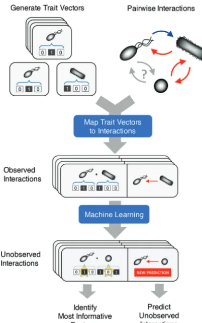
concatenation of the relevant trait vectors (Fig. 1). Trait vectors may be constructed
from any set of biologically relevant features, such as the presence/absence of a certain
gene or metabolic function, phylogenetic classifications, or even characteristics of the
environment where the organism was found. In our analyses, different case studies
were based on different trait vector representations: in particular, we used (i) the
on September 8, 2020 by guest
presence/absence of metabolic reactions for the
in silico
community case study, (ii)
binary vectors of biosynthetic capabilities for each
E. coli
strain in the auxotroph
community case study, and (iii) metabolic functions predicted from 16s sequences for
the soil community case study.
These trait vectors, together with the known outcome of a subset of interactions,
can be fed into machine learning algorithms that separate outcome classes and
subsequently predict the outcome of unobserved interactions. Here, we used the
random forest algorithm, based on an ensemble of many decision trees that
individ-ually ask a series of yes or no questions about randomly selected subsets of predictive
features to classify samples. To find potential mechanisms of interaction, we took
advantage of the structure of individual trees to identify which variables are the most
influential for the classification of specific samples.
Application to computationally predicted interactions between human gut
microbes.
We first applied our approach to a large
in silico
data set generated by
simulating time course microbial coculture experiments with dynamic flux balance
analysis (23, 24) using Computation of Microbial Ecosystems in Time and Space
(COMETS) (5) (see Materials and Methods). The dynamic flux balance analysis enables
the computation of approximate growth curves on the basis of the complete metabolic
FIG 1 Schematic representation of our machine learning approach for inferring interactions among microbes. A trait vector captures the characteristics of each organism in the community of interest. The presence or absence of a trait in a given organism is encoded (as a binary number) in the corresponding element of the trait vector. For every possible pairwise interaction among community members, we construct a composite vector that is the concatenation of the corresponding trait vectors. The vector of the organism whose response is being predicted is concatenated to the front of the trait vector of its interaction partner. For the set of observed interactions, each composite vector is then mapped to the measured response of the interacting species. All observed interactions are then used to train a model that predicts the outcome of unobserved interactions. If random forest is used, then feature contribu-tions can be calculated on a case-by-case basis to identify which elements of the composite genome contribute most strongly to the prediction.on September 8, 2020 by guest
http://msystems.asm.org/
networks of the microbes (derived from their sequenced genomes) and the abundance
of each nutrient present in the medium at the beginning of the experiment. The
simulated experiment provides an estimate of the final biomass for each organism and
the exchange fluxes during exponential growth. The possible interactions between
different species in the coculture may result from the exchange of secreted by-products
or the competition for common nutrients. To generate a large set of observations for
machine learning, we selected metabolic models of 100 human gut-associated bacteria
(25) and used COMETS to simulate all pairwise coculture interactions within the same
rich medium in a well-mixed batch culture scenario.
The trait vectors used to represent each organism were simply binary vectors
indicating the presence or absence of various nutrient exchange reactions in the
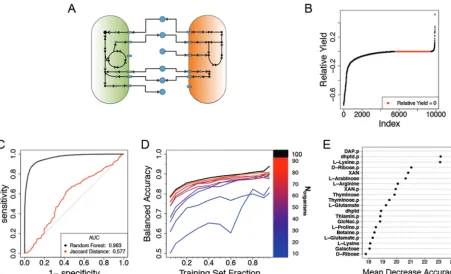
metabolic network models (see Materials and Methods and Fig. 2A). The interactions in
the network were computed by determining the influence of every organism on every
other organism in COMETS coculture simulations. In particular, the simulations
pro-vided the final biomass of each organism in coculture and in monoculture. A
normal-ized difference between these two yields (i.e., the relative yield; see Materials and
Methods) was used as the phenotypic metric for classifying the interaction (negative or
nonnegative) (Fig. 2B).
The random forest algorithm was first applied to the full data set, revealing that its
out-of-bag (OOB) accuracy (roughly equivalent to a 5-fold cross-validation; see
refer-FIG 2 Classification of pairwise interactions for anin silicomodel of a community of human gut microbes. (A) Organisms are representedin silico
as large networks of metabolic reactions that take up metabolites (blue circles) from the environment (arrows leading to model) and release by-products (arrows leading to metabolite). Organisms may interact with one another during the simulation when both organisms compete for the uptake of a metabolite or through cross feeding, where one model consumes a by-product of the other. (B) Relative yields from all experiments are plotted in ascending order. There were 5,563 samples with a negative relative yield. Neutral interactions, a relative yield of zero,
occurred 3,917 times, and positive relative yield occurred 420 times. Samples were classified as negative or nonnegative. (C) For all 9,900in silico
observations, the ROC curve of a random forest classifier was determined by using 388 exchange reactions as predictors and compared to the ROC curve obtained from using the Jaccard distance as a simple threshold to predict negative versus nonnegative relative yields. Values for the ROC curve were obtained by evaluating the class voting ratios on out-of-bag samples (see Materials and Methods). ROC curves for classifiers
trained on subsets of the data can be seen in Fig. S3 in the supplemental material. (D) Learning curves for subcommunities of the fullin silico
community. These learning curves are the median learning curves evaluated with 10-fold cross-validation on test sets at each point (see Materials
and Methods) for 5 subcommunities selected at random for each value ofNorganisms. (E) A representation of the 20 most influential predictors as
determined by mean decrease in accuracy. Labels on theyaxis indicate the feature names. A “p” suffix in the label indicates that the predictor
is a feature of the interaction partner; DAP, meso-2,6-diaminopimelate; dhptd, 4,5-dihydroxy-2,3-pentanedione; XAN, xanthine; GlcNac,
N-acetylglucosamine. The results of an alternative representation scheme using phylogenies are presented in Fig. S5.
on September 8, 2020 by guest
ence 26 and Materials and Methods) was approximately 90.5%. The receiver operator
characteristic (ROC) curve for the random forest algorithm (Fig. 2C and Materials and
Methods) compares favorably to a naive prediction based on the Jaccard distance (27)
between the different trait vectors (see Materials and Methods and see references 28
and 29 for similar use of Jaccard distance in microbial community studies).
The high predictive accuracies are encouraging but are of little use if they can only
be achieved when the vast majority of the experiment outcomes are already known.
Thus, we constructed a series of learning curves to visualize how the balanced accuracy
of the random forest classifier is affected by the size of the community and by the
amount of training data available (Fig. 2D). For small communities (for example,
N
organisms⫽
10), there is little gain in predictive performance until the experimental
space is nearly totally known. However, when
N
organismsis increased to 20 (which
amounts to 190 pairwise experiments, corresponding to 380 individual responses to
coculture), as little as 5% of the total data (
⬃
9 to 10 experiments, i.e., 18 to 20
responses) is sufficient to obtain useful predictions. The ROC curves and comparison
with a Jaccard distance classifier for selected points along the learning curve showed
a similar trend to what seen for the full data set (see Fig. S3 in the supplemental
material). The general trend indicates that the larger a community is, the smaller the
relative fraction of experiments needed to obtain a high accuracy. In general, learning
curves can be used as guidelines to determine how many experiments should be
implemented to reach a target performance.
In addition to confirming that the algorithm accurately classifies unobserved
inter-actions, we investigated whether the top feature vector components used as the
predictors are biologically interpretable. The variable importance plot (see Materials
and Methods and Fig. 2E) shows the globally most informative trait vector components.
In this case, the most important predictor for the classification of a given organism was
a feature of the interaction partner (Fig. 2E). In other words, the predicted growth
phenotype of organism
i
in the presence of organism
j
is best described by features that
are in the vector for organism
j
. In addition to analyzing the global contributions of
variables to the classifications across all data, the tree-based approach of random
forests can be used to determine why specific samples were classified as they were by
examining the feature contributions for specific interactions. A feature contribution (see
details in Materials and Methods) quantifies how much a given variable typically
influences the classification probability of a single sample. Feature contributions were
originally developed for the analysis of regression models (30) but have since been
adapted for binary classification models (22). We wondered whether the simulated data
could be used to illustrate the possible value of feature contributions for identifying
putative biological mechanisms underlying a given interaction. In particular, we
envis-aged that the random forest algorithm, trained only on the basis of the trait profiles and
the relative yields in cocultures, could be used to suggest which metabolites may be
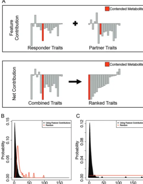
more likely to mediate a given competitive (Fig. 3) or facilitative (see Fig. S1) interaction.
As opposed to an
in vitro
system, where such a prediction would need to be validated
with new experiments, our
in silico
system enables the value of the random forest
prediction to be checked by comparing it with simulated exchange fluxes across the
two species (which, importantly, were not used in training the random forest).
Towards this goal, for each pair of organisms, we ranked— by their net feature
contributions (see Materials and Methods, Fig. 3A, and Table S1)—the 194 metabolites
involved in exchange reactions. We found that the metabolites ranking highly on the
basis of this criterion were much more likely than random to be among the metabolites
truly exchanged in the COMETS simulations (Fig. 3B). This is particularly valuable if the
interaction is due to a single exchanged metabolite (Fig. 3C). In practice, if this criterion
was used on
in vitro
data, it would imply a significant reduction in the number of tests
needed to identify at least one mechanism of interaction.
It is also instructive to look in more detail at a specific case of feature contribution
analysis. In particular, we observed that fructose exchange was most frequently the
strongest predictor of competitive interactions (it was the top ranking true feature in
on September 8, 2020 by guest
http://msystems.asm.org/
⬃
18.7% of all competitive interactions) (Table S1), and it corresponded to the 15th
most common true mechanism based on the COMETS-simulated fluxes (see Table S2).
Interestingly, fructose has been implicated in altering the gut microbiome in a number
of diseases, including antibiotic-treatable metabolic syndrome (31–33), liver disease
(34), and obesity (35). Our approach is also readily applicable for the discovery of
metabolites that mediate positive interactions, which comprise a small minority of all
interactions (420/9,900). Due to the scarcity of their occurrence and the dearth of
metabolites that mediate positive interactions, the discovery of these mechanisms is
more challenging. Nevertheless, the use of ranked feature contributions to find the
facilitative metabolites was a powerful improvement over a naive approach (Fig. S1).
Application to a community of auxotrophic
Escherichia coli
strains.
We next
applied the random forest algorithm to experimental data on auxotrophic
E. coli
cocultures. In particular, we used previously published data from all possible cocultures
of 14
E. coli
strains, each auxotrophic for a given amino acid (36). The interactions
between any given pair of
E. coli
strains are presumably dependent on the direct
FIG 3 Using feature contributions to find a metabolite for which two organisms compete. (A) Metabolite transporters belonging to the organism of interest (top left) or the interaction partner (top right). We were interested in identifying a metabolite that is associated with the negative relative yield for the organism of interest. To establish a ranking of metabolites, the feature contributions from both of the composite trait vectors (top) were summed and sorted according to the net contribution (bottom). Proceeding from the negative end, the rank and identity of the first contended metabolite encountered relative to the negative end of the new vector was recorded. (B) The probability distributions of the average rank at which the first mechanistic metabolite is encountered by sampling metabolites randomly one at a time calculated for each sample and for feature contributions. By chance, the first metabolite is encountered after 13 random queries. Feature contributions reduce the median number of queries to 4. (C) Ninety-nine samples produced a negative relative yield through the competition for one metab-olite. Randomly investigating each of the 194 candidate metabolites results in an average of 97.5 experiments before discovering the metabolite. By using feature contributions to prioritize the order in which to investigate metabolites, the contended metabolite is revealed on or before the fourthexperiment (median⫽4).
on September 8, 2020 by guest
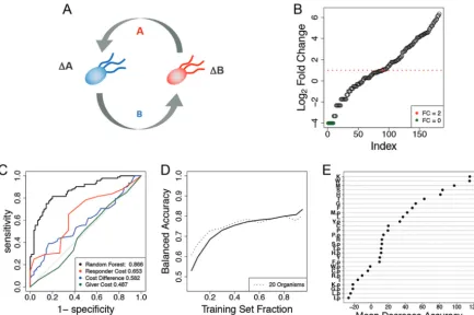
exchange of the missing amino acids or related precursors (Fig. 4A). The total growth
of each strain in the 91 experiments was measured after 84 h and reported as the net
fold change relative to the initial inoculum, resulting in 182 total observations (see
Materials and Methods for additional comments on the experimental setup). We built
trait vectors according to the 14 amino acids and labeled growth phenotypes according
to the fold change response of a given
E. coli
auxotroph strain in coculture with another
auxotrophic strain (using 2 as the fold change cutoff for distinguishing between
“strong” and “weak” interaction phenotypes) (Fig. 4B).
The random forest algorithm yielded a balanced accuracy of
⬃
79.2% in predicting
this interaction phenotype. An examination of the corresponding ROC curves showed
that the random forest is a much better predictor than simpler metrics based on
biosynthetic costs (36) of the different amino acids (Fig. 4C). The learning curve for this
test case (Fig. 4D) resembles the trajectory of the learning curve for
in silico
commu-nities of 20 members (Fig. 2D). The variable importance rankings show that, in general,
the amino acid needed by the receiver has a greater impact on the classification
accuracy than the amino acid its partner needs, suggesting that the specificity of the
interaction is dominated by auxotrophies, whereas most mutants can, in principle,
provide the missing amino acid (Fig. 4E).
As done for the
in silico
simulations, we next analyzed the feature contributions and
asked whether they reflect the underlying mechanisms. In particular, we asked how
FIG 4 Data representation and results for the case study of a network of auxotrophicE. colistrains. (A) In the original experiment,
single-gene knockoutE. coliauxotrophs were cocultured in minimal medium. For the ΔA mutant to grow, it must receive amino acid A
from the ΔB mutant, which in turn must receive another amino acid, B, for growth. Auxotroph strains were constructed for the following amino acids: cysteine, phenylalanine, glycine, histidine, isoleucine, leucine, methionine, proline, arginine, serine, threonine, tryptophan,
and tyrosine. (B) Auxotroph strain fold changes in ascending order.E. colistrains had a weak response (fold changeⱕ2) 90 times and
failed to grow 9 times (green circles). In 92 instances, theE. coliauxotroph population more than doubled over the course of 84 h. (C)
ROC curves for all 182 observations were determined for a random forest classifier using 28 amino acids as predictors. Single-value thresholds based on the biosynthetic costs of knocked-out amino acids resulted in poorer performance than the random forest algorithm.
(D) Trajectory of a learning curve built for theE. coliinteractions (solid line) closely resembles that of the learning curve forin silico
communities with 20 organisms (dashed line). (E) Ranking of 28 amino acids according to their effects on prediction accuracy when randomly permuted. Amino acids corresponding to the receiver strain are enriched near the top of the list. A suffix “p” indicates that the predictive feature belongs to the giver strain. A single case of a Δmethionine mutant cocultured with a Δcysteine mutant is shown in Fig. S2.
on September 8, 2020 by guest
http://msystems.asm.org/
often the absence of one of the two amino acids for a pair of organisms has the
strongest contribution in the random forest algorithm. As expected, the random forest
algorithm is more strongly influenced by the absence of an amino acid feature than by
its presence. Of all 182 observations, the absence of the amino acid from the receiver
had the largest feature contribution 140 times, and the absence of the amino acid from
the giver had the largest contribution 40 times (see Table S3). Thus, the pair of most
influential predictors tended to correspond to the underlying mechanism of the
interaction, even in instances where the predicted class was incorrect. Scenarios where
the presumed mechanisms are the strongest contributors sometimes resulted in
mis-classification, presenting opportunities for direct research of interesting outliers. The
response of the methionine auxotroph (ΔMet mutant) in coculture with the cysteine
auxotroph (ΔCys mutant) was one such case, which we describe in detail in Fig. S2.
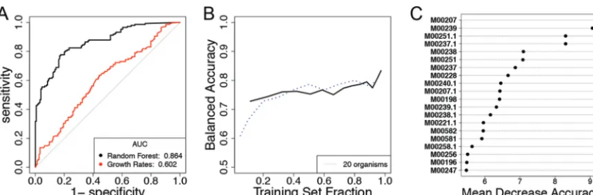
Application to a community of soil bacteria.
For the final test case, we analyzed
the results of a study featuring all pairwise coculture experiments of 20 bacterial strains
isolated from the same soil sample (3) (see Materials and Methods). For each
experi-ment, the authors reported whether each species was present at a detectable level at
the final time point. We built trait vectors according to the presence or absence of KEGG
modules (37) as predicted by PICRUSt (38). The random forest algorithm trained on the
full data set provided an out-of-bag balanced accuracy of 79.4%. The ROC curve shows
that the random forest algorithm performed much better than a simple decision rule
based on the differences in the reported initial growth rates of each species (Fig. 5A).
The learning curve for this community closely resembles that of the 20-member
communities from our
in silico
case study (Fig. 5B). The variable importance plot shows
that the predictions were most strongly influenced by the transport of teichoic acids
(which are found in the walls of several Gram-positive bacteria [39]), both in the strain
being predicted and in its interaction partner (Fig. 5C, see also Table S4 for KEGG
module names). Further insight into relevant pair-specific KEGG modules can be
obtained from feature contributions (see Table S5).
DISCUSSION
Exhaustive pairwise coculture studies of microbial strains are an increasingly
com-mon avenue for estimating an ecosystem interaction network. While such pairwise
interactions do not necessarily capture all possible interdependencies in a community
(4, 40), they have been shown to be a dominant factor (12), making the reliable
prediction and interpretation of predictive models matters of great importance. In this
study, we described a conceptual framework for the representation of microbes and
their pairwise interactions to address both of these challenges.
The ideal data sets for testing our approach would include a large number of pairs
FIG 5 (A) ROC curves from the random forest trained on all 302 observations using 79 predicted KEGG modules as features. The difference in the initial growth rates of both strains was used as a baseline simple predictor. (B) The learning curve built on this data set starts at
⬃72% balanced accuracy and tops out at⬃78% balanced accuracy (solid line). The learning curve for thein silicocommunities with 20
organisms is displayed for comparison (dashed line). (C) The identifiers (IDs) of the most important modules for predictive accuracy of the forest. See Table S4 for the full module names.
on September 8, 2020 by guest
of microbes and genotypes or multidimensional phenotypes for each species. While we
envisage that a multitude of such data sets will be available in the future, the existing
data sets are either limited in size or in trait vector accessibility. Thus, we tested our
approach on three data sets, each with a different set of advantages and limitations.
The first and largest data set was obtained by simulating 4,950 microbial cocultures
with dynamic flux balance metabolic modeling (COMETS). An important caveat about
this specific test case is that metabolic models may not capture the full biochemical
details of the real system they approximate, and they do not incorporate any of the
nonmetabolic processes that may be observed in real communities (41). However,
these models have been used to successfully help understand the physiology of
specific organisms (42) and communities (5, 43, 44). The other two experimental studies
we used were not affected by these issues, but they were limited in the numbers of
organisms and pairs analyzed. The first experimental data set was the outcome of a
study involving 14 strains of
E. coli
amino acid auxotrophs. In this case, the trait vectors
were a straightforward representation of the auxotrophies, but the random forest
algorithm highlighted the complexity of the underlying interdependencies. The second
experimental data set was from a community of soil microbes, whose trait vectors were
derived from the available 16s rRNA sequences, suggesting a broad applicability of our
approach to future similar studies.
The qualitative prediction of the outcome of unobserved interactions is most
valuable if that prediction leads to a reduction in the usage of precious resources and
time. To this end, the construction of learning curves is an important step in identifying
how much data are required to achieve the desired prediction accuracy from machine
learning. This may be particularly useful for planning large-scale studies of naturally
cooccurring species or synthetic consortia, e.g., for searching communities with specific
properties relevant for biomedical or engineering applications (45).
Despite the common perception that random forest algorithms are merely
uninter-pretable “black boxes,” we showed here that feature contributions provide a clear
window into the decision-making process of a random forest. If the features are defined
on the basis of clearly identifiable biological entities (e.g., genes, reactions, or
pheno-typic traits), then the feature contributions can be effectively used to guide
experi-ments that help reveal the underlying mechanisms.
In the current implementation of our algorithm, we concatenated the binary trait
vectors of two organisms to form a new composite trait representation. However,
alternative representations of microbes and their interactions are possible and should
be explored. These may also include more quantitative information, such as the gene
copy number or the mean transcriptional levels. While in our current work the
envi-ronment for each case study was fixed, it is also possible to apply our method to data
from heterogeneous environments, provided that the environmental parameters are
encoded in the trait vector.
The present study focused entirely on demonstrating the possible benefits of
applying machine learning to the study of interspecies interactions in microbial
com-munities. In this context, our use of mechanistic models (based on dynamic flux balance
analysis) was limited to the generation of
in silico
data sets meant to enable the testing
of our approach. However, we envisage that in the future it will be possible to integrate
machine learning and mechanistic approaches toward a better characterization and
design of microbial consortia. More broadly, we foresee that the interplay of
quanti-tative approaches with high-throughput genotypic and phenotypic measurements will
constitute a very valuable instrument for future microbiome research and synthetic
ecology.
MATERIALS AND METHODS
Representation of interactions with trait-derived features.For a given communityC, the
ob-served coculture response of each speciesiin the presence of speciesjis encoded in the elementXijof
a community matrixX.Xijrepresents the appropriately normalized abundance of speciesiat the end of
a coculture experiment with speciesjor a binary variable describing whether or not speciesiwill survive
after inoculation with speciesj. To define a set of trait vectors for each organism inC, a list ofnfeatures
on September 8, 2020 by guest
http://msystems.asm.org/
present in an organism, including uptake/secretion. Flux balance analysis (FBA) is a constraint-based steady-state approach that uses this stoichiometry to predict fluxes and growth capacity under a given boundary condition of nutrient availability and has been described in detail (24, 41, 43, 46). Briefly, the set of reactions contained in a model is derived from the organism’s genome annotation. The reactions
are then used to construct the stoichiometric matrix Sfor the metabolic model, whose elementSij
indicates the number of molecules of typeiused or produced by reactionj. The identification of feasible
metabolic fluxes (v) for the system is achieved by imposing a steady state (Sv⫽0), as well as upper/lower
bound constraints that define the environmental nutrient availability. Standard flux balance analysis calculations then use linear optimization to identify feasible flux states that maximize a given objective function, usually the growth flux of the cell, i.e., the production of a balanced biomass composition of the organism.
Dynamic flux balance analysis (dFBA) (23) extends the classical FBA to perform dynamic simulations in which intracellular metabolites are still assumed to be at steady states but total biomass and environmental metabolites are treated as time-dependent variables in a discretized approximation. Crucially, in a dFBA simulation of multiple species, competition or facilitation (e.g., cross feeding) are
emergent properties of the flux dynamics of individual organisms. Thus, noa prioriassumptions need to
be made about the existence or nature of the ecological interactions. dFBA simulations were performed using our platform for Computation of Microbial Ecosystems in Time and Space (COMETS), which was previously used to model microbial communities (5). One hundred metabolic models (25) were selected, and a common medium that enables the growth of nearly all models in a monoculture scenario was identified. Pairwise coculture simulations of the 100 models were performed by using the common medium in a well-mixed batch culture scenario (approximated by using COMETS without spatial structure). For each scenario, the biomass accumulation and fluxes were used to calculate the relative
yield and identify the mechanisms of interaction, respectively. In this case,Xijcorresponds to the relative
yield of strainiin coculture with strainjat the final time point.Xijcan be directly computed from the
amounts of biomass for different species at the end of the COMETS simulations. IfBijis the final amount
of biomass for organismiin coculture with organismj, and the diagonal elementBiiis the biomass ofi
in monoculture, then the relative yield is defined asXij⫽共Bij⫺Bii兲⁄Bii, where anXijof⬍0 indicates strain
i(i.e., the responder) is detrimentally affected by its partner. Correspondingly, anXijof 0 indicates no
effect and anXijof⬎0 indicates a positive effect ofjoni.
For this case study, the feature profileF共i兲for speciesiencodes the presence (1) or absence (0) of each
of 194 possible exchange reactions (corresponding to the columns in theSmatrix). It is important to note
that these feature vectors are equivalent to functional annotations based on genomes, e.g., the profiles of the presence/absence of specific genes. They do not depend on the fluxes that can be eventually computed for each of the corresponding reactions.
In addition to implementing the random forest algorithm, as described below in “Implementation of random forest,” a simple classifier was built on the basis of the Jaccard distance (JD) between two feature vectorsF(i)andF(j), defined as
JD
共
F(i),F(j)兲
⫽1⫺共
F(i)艚F(j)兲
⁄共
F(i)艛F(j)兲
.Data for case study of auxotrophicE. coli.The measured growth responses of individualE. coli
strains and biosynthetic costs of amino acids were obtained from the supplemental files provided in
reference 36. In that study, 14 strains of amino acid auxotrophicE. coliwere generated by knocking out
single genes. The cocultures were reported as being inoculated in 200l of M9 glucose medium in
96-well microtiter plates at an initial cell density of 107cells/ml and incubated at 30°C for 84 h, at which
point the fold change in growth relative to the initial inoculum for each strain was determined by plating, counting colonies, and quantitative PCR (qPCR) to identify strain proportions. In this case, the feature
vectorF(i)(lengthn⫽14) encodes the presence/absence of biosynthetic capabilities for each of the 14
amino acids, and the coculture phenotypeXijcorresponds to the fold change of strainiin coculture with
strainjat the final time point, which may represent the final growth yield. On the basis of the original
data set, batch effects (e.g., evaporation) or mutations did not affect the quantitative estimate of the reported yield and thus the outcome of our analysis. However, a further scrutiny of the level of precision in yield measurements and corresponding estimates of how experimental errors might affect machine learning outcomes would be an important subject for future follow-up studies.
Data for case study of soil community.The results of an experimental study of 20 soil microbial strains in which all pairwise coculture experiments were performed in a yeast extract nutrient broth
on September 8, 2020 by guest
medium were obtained (3). The survival of different strains after 5 dilution cycles was estimated by plating coculture medium and counting colonies and was verified with next-generation sequencing. For
our analysis, Xijencoded the reported persistence (Xij⫽ 1) or exclusion (Xij⫽ 0) of strain iwhen
cocultured with strainj. To generate feature vectorsF(i)for this community, the 16s rRNA sequence of
each strain was downloaded from GenBank (47), and PICRUSt (38) was used to predict the presence of KEGG modules. The KEGG modules for 18 strains were obtained, and each strain was represented by a binary trait vector of 79 modules (see Table S4 in the supplemental material).
Implementation of random forest.We used the randomForest R library (26). Random forests are ensemble classifiers that aggregate the results of many individual decision trees. This specific algorithm utilizes two hyperparameters: the number of training trees (nTree) and the number of predictors to
consider at each split point (mTry). The default settings of nTree and mTry were near optimal for ourin
silicodata set (Fig. S4); therefore, only the default settings were used for the remainder of the study. Each tree in the random forest was assigned a synthetic data set that is of the same size as the training set but generated through sampling with replacement. The average tree was thus trained on approximately two-thirds of the observations; these observations are referred to as in-bag samples. The remaining one-third of the observations not in the synthetic data sets are referred to as out-of-bag samples. The new synthetic data set was placed at the root node of a new tree; next, a randomly selected subset of predictive features was queried for the best split of the data into two child nodes. This process was repeated at each node until a stop criterion was met. The classification accuracy of individual trees was assessed by using them to predict their out-of-bag samples and recording the results. The random forest then makes a classification call for individual samples according to the class predicted by the majority of the trees. The accuracy was evaluated on the full training set with out-of-bag performance metrics and has been shown to be equivalent to 5-fold cross-validation (26). The ratio of the votes of the out-of-bag trees was used to construct ROC curves (see “ROC curves” below). See reference 19 for a full description of the algorithm.
Balanced accuracy.The balanced accuracy for evaluating the performance of classifiers on inde-pendent test sets and on the OOB samples when the model was trained using the full data set is reported. This metric is based on the values from the confusion matrix: true positive (TP), true negative
(TN), false positive (FP), and false negative (FN). The balanced accuracy is calculated as [TP/(TP⫹FN)⫹
TN/(TN⫹FP)]/2.
ROC curve.To evaluate the random forest classifiers for each case study, the receiver operator curve (ROC) from the model trained on the full set of available data was determined. Using the out-of-bag
voting proportions, the true-positive rate (sensitivity) was plotted against the false-positive rate (1⫺
specificity) as the classification threshold was increased from the minimum value to the maximal value. In the context of the random forest algorithm, the classification threshold is the fraction of out-of-bag votes for the positive class. After generating the ROC curve, the area under the curve (AUC) as calculated with the “AUC” package in R (48).
Learning curves.To construct the learning curves, a set of fractions was defined,r⫽[0.05, 0.1, 0.2, 0.3, 0.4, 0.5, 0.6, 0.7, 0.8, 0.9, 0.95], for evaluating the balanced accuracy of the model using
cross-validation. For all cross-validation experiments, observationsXijandXjiwere both either in the training
set or in the test set. For each fraction inr, a subset of the community matrix of the corresponding size
was randomly selected to use as a training set and the remaining data were reserved as an independent test set. This process was repeated until at least 10 subsets of training data were selected for each value
inr. The median balanced accuracy of classifiers was then calculated for each fraction. To investigate the
effect of the community size on the learning curve, a set of community sizes was defined (c⫽[10, 20,
30, 40, 50, 60, 70, 80, 90]). For each community size inc, five community submatrices were randomly
selected from the fullin silicocommunity matrix. Then, the learning curve was determined for each
subcommunity. For each size inc, the median learning curve for balanced accuracy of each community
size was calculated and is reported in Fig. 2D.
Variable importance plots.Variable importance plots are commonly used with random forests to evaluate which variables are the most important for the model by comparing their mean decrease in accuracy scores. The mean decrease in accuracy is a measurement of the change in the accuracy of the forest’s predictions when the variable in question is randomly permuted (20). Here, it was used for the relative ranking of the global importance of each feature. The randomForest package automatically generates the variable importance plots, which are shown in Fig. 2E, 4E, and 5C.
Feature contributions for binary classifications.The calculation of feature contributions was de-scribed previously (22). This calculation quantifies the effect of a given variable on the classification of a
specific samplej. After the training of a random forest withTtrees, the number of training samples
at nodekthat belong to each of the two classes (C1and C2) can be counted for each treetand node
kin the path followed by samplejin treet. The fraction of samples belonging to C1is indicated by
Yt,kj . The following steps are performed to evaluate the contribution of an individual featurefin
classifying a specific sample. (i) At each node where feature fis the splitting variable, the local
increment (Lt,k,f j
) in the fraction of samples belonging to class C1is calculated asLt,k,f
j ⫽Y t,k⫹1 j ⫺ Y
t,k j
. (ii) The
mean sample-specific contribution of a given featurefacross all trees is obtained by averaging over all the
local increments, i.e.,
fj⫽
冘
t⫽1 TLt,k,fj
T
on September 8, 2020 by guest
http://msystems.asm.org/
FIG S5
, PDF file, 0.01 MB.
TABLE S1
, PDF file, 0.04 MB.
TABLE S2
, PDF file, 0.02 MB.
TABLE S3
, PDF file, 0.04 MB.
TABLE S4
, PDF file, 0.03 MB.
TABLE S5
, PDF file, 0.1 MB.
ACKNOWLEDGMENTS
We thank Jenny Bhatnagar and Carolyn Zeiner, whose work with fungal interactions
served as the initial inspiration for this study, and the members of the Segrè lab for
helpful discussions and for feedback on the manuscript.
D.S. and D.D. received funding from the Defense Advanced Research Projects
Agency (purchase request no. HR0011515303, contract no. HR0011-15-C-0091), the
Army Research Office under MURI award W911NF-12-1-0390, the U.S. Department of
Energy (DE-SC0012627), the NIH (T32GM100842, 5R01DE024468, R01GM121950, and
Sub_P30DK036836_P&F), the National Science Foundation (1457695), the Human
Fron-tiers Science Program (RGP0020/2016), and the Boston University Interdisciplinary
Biomedical Research Office.
REFERENCES
1. Røder HL, Sørensen SJ, Burmølle M. 2016. Studying bacterial
multispe-cies biofilms: where to start? Trends Microbiol 24:503–513.https://doi
.org/10.1016/j.tim.2016.02.019.
2. Aziz FAA, Suzuki K, Ohtaki A, Sagegami K, Hirai H, Seno J, Mizuno N, Inuzuka Y, Saito Y, Tashiro Y, Hiraishi A, Futamata H. 2015. Interspecies interactions are an integral determinant of microbial community
dynam-ics. Front Microbiol 6:1148.https://doi.org/10.3389/fmicb.2015.01148.
3. Higgins LM, Friedman J, Shen H, Gore J. 2017. Co-occurring soil bacteria exhibit a robust competitive hierarchy and lack of non-transitive
inter-actions. bioRxivhttps://doi.org/10.1101/175737.
4. Bairey E, Kelsic ED, Kishony R. 2016. High-order species interactions
shape ecosystem diversity. Nat Commun 7:12285. https://doi.org/10
.1038/ncomms12285.
5. Harcombe WR, Riehl WJ, Dukovski I, Granger BR, Betts A, Lang AH, Bonilla G, Kar A, Leiby N, Mehta P, Marx CJ, Segrè D. 2014. Metabolic resource allocation in individual microbes determines ecosystem
inter-actions and spatial dynamics. Cell Rep 7:1104 –1115.https://doi.org/10
.1016/j.celrep.2014.03.070.
6. Coyte KZ, Schluter J, Foster KR. 2015. The ecology of the microbiome:
networks, competition, and stability. Science 350:663– 666.https://doi
.org/10.1126/science.aad2602.
7. Taga ME, Bassler BL. 2003. Chemical communication among bacteria.
Proc Natl Acad Sci U S A 100:14549 –14554.https://doi.org/10.1073/pnas
.1934514100.
8. Datta MS, Sliwerska E, Gore J, Polz MF, Cordero OX. 2016. Microbial interactions lead to rapid micro-scale successions on model marine
particles. Nat Commun 7:11965.https://doi.org/10.1038/ncomms11965.
9. Johns NI, Blazejewski T, Gomes ALC, Wang HH. 2016. Principles for designing synthetic microbial communities. Curr Opin Microbiol 31:
146 –153.https://doi.org/10.1016/j.mib.2016.03.010.
10. Shou W, Ram S, Vilar JMG. 2007. Synthetic cooperation in engineered
yeast populations. Proc Natl Acad Sci U S A 104:1877–1882.https://doi
.org/10.1073/pnas.0610575104.
11. Zomorrodi AR, Segrè D. 2016. Synthetic ecology of microbes:
mathe-matical models and applications. J Mol Biol 428:837– 861.https://doi
.org/10.1016/j.jmb.2015.10.019.
12. Venturelli OS, Carr AC, Fisher G, Hsu RH, Lau R, Bowen BP, Hromada S, Northen T, Arkin AP. 2018. Deciphering microbial interactions in syn-thetic human gut microbiome communities. Mol Syst Biol 14:e8157.
https://doi.org/10.15252/msb.20178157.
13. Friedman J, Higgins LM, Gore J. 2017. Community structure follows simple assembly rules in microbial microcosms. Nat Ecol Evol 1:109.
https://doi.org/10.1038/s41559-017-0109.
14. Goers L, Freemont P, Polizzi KM. 2014. Co-culture systems and technologies: taking synthetic biology to the next level. J R Soc Interface
11:20140065.https://doi.org/10.1098/rsif.2014.0065.
15. Lasken RS, McLean JS. 2014. Recent advances in genomic DNA sequenc-ing of microbial species from ssequenc-ingle cells. Nat Rev Genet 15:577–584.
https://doi.org/10.1038/nrg3785.
16. Gawad C, Koh W, Quake SR. 2016. Single-cell genome sequencing:
current state of the science. Nat Rev Genet 17:175–188.https://doi.org/
10.1038/nrg.2015.16.
17. Seemann T. 2014. Prokka: rapid prokaryotic genome annotation.
Bioin-formatics 30:2068 –2069.https://doi.org/10.1093/bioinformatics/btu153.
18. Dam P, Olman V, Harris K, Su Z, Xu Y. 2007. Operon prediction using both genome-specific and general genomic information. Nucleic Acids Res
35:288 –298.https://doi.org/10.1093/nar/gkl1018.
19. Ho TK. 1995. Random decision forests, p 278 –282. Proceedings of 3rd International Conference on Document Analysis and Recognition, Mon-treal, Canada.
20. Breiman L. 2001. Random forests. Mach Learn 45:5–32.https://doi.org/
10.1023/A:1010933404324.
on September 8, 2020 by guest
21. Liaw A, Wiener M. 2002. Classification and Regression by randomForest. R News 2:18 –22.
22. Palczewska A, Palczewski J, Robinson RM, Neagu D. 2013. Interpreting random forest classification models using a feature contribution method (extended). 2013 IEEE 14th Int Conf Inf Reuse Integr, San Francisco, CA. 23. Henson MA, Hanly TJ. 2014. Dynamic flux balance analysis for synthetic
microbial communities. IET Syst Biol 8:214 –229.https://doi.org/10.1049/
iet-syb.2013.0021.
24. Maarleveld TR, Khandelwal RA, Olivier BG, Teusink B, Bruggeman FJ. 2013. Basic concepts and principles of stoichiometric modeling of
met-abolic networks. Biotechnol J 8:997–1008.https://doi.org/10.1002/biot
.201200291.
25. Bauer E, Laczny CC, Magnusdottir S, Wilmes P, Thiele I. 2015. Phenotypic differentiation of gastrointestinal microbes is reflected in their encoded
metabolic repertoires. Microbiome 3:55.https://doi.org/10.1186/s40168
-015-0121-6.
26. Svetnik V, Liaw A, Tong C, Culberson J, Sheridan RP, Feuston BP. 2003. Random Forest: a classification and regression tool for compound clas-sification and QSAR modeling. J Chem Inf Comput Sci 43:1947–1958.
https://doi.org/10.1021/ci034160g.
27. Jaccard P. 1912. The distribution of the flora in the Alpine zone. New
Phytol 11:37–50.https://doi.org/10.1111/j.1469-8137.1912.tb05611.x.
28. Bach EM, Williams RJ, Hargreaves SK, Yang F, Hofmockel KS. 2018. Greatest soil microbial diversity found in micro-habitats. Soil Biol
Biochem 118:217–226.https://doi.org/10.1016/j.soilbio.2017.12.018.
29. Mainali KP, Bewick S, Thielen P, Mehoke T, Breitwieser FP, Paudel S, Adhikari A, Wolfe J, Slud EV, Karig D, Fagan WF. 2017. Statistical analysis of co-occurrence patterns in microbial presence-absence datasets. PLoS
One 12:e0187132.https://doi.org/10.1371/journal.pone.0187132.
30. Kuz’min VE, Polishchuk PG, Artemenko AG, Andronati SA. 2011. Inter-pretation of QSAR models based on Random Forest methods. Mol
Inform 30:593– 603.https://doi.org/10.1002/minf.201000173.
31. Di Luccia B, Crescenzo R, Mazzoli A, Cigliano L, Venditti P, Walser JC, Widmer A, Baccigalupi L, Ricca E, Iossa S. 2015. Rescue of fructose-induced metabolic syndrome by antibiotics or faecal transplantation in
a rat model of obesity. PLoS One 10:e0134893.https://doi.org/10.1371/
journal.pone.0134893.
32. Khitan Z, Kim DH. 2013. Fructose: a key factor in the development of metabolic syndrome and hypertension. J Nutr Metab 2013:682673.
https://doi.org/10.1155/2013/682673.
33. Bantle JP. 2009. Dietary fructose and metabolic syndrome and diabetes.
J Nutr 139:1263S–1268S.https://doi.org/10.3945/jn.108.098020.
34. Lambertz J, Weiskirchen S, Landert S, Weiskirchen R. 2017. Fructose: a dietary sugar in crosstalk with microbiota contributing to the develop-ment and progression of non-alcoholic liver disease. Front Immunol
8:1159.https://doi.org/10.3389/fimmu.2017.01159.
35. Payne AN, Chassard C, Lacroix C. 2012. Gut microbial adaptation to dietary consumption of fructose, artificial sweeteners and sugar alcohols: implications for host-microbe interactions contributing to
obe-sity. Obes Rev 13:799 – 809. https://doi.org/10.1111/j.1467-789X.2012
.01009.x.
36. Mee MT, Collins JJ, Church GM, Wang HH. 2014. Syntrophic exchange in synthetic microbial communities. Proc Natl Acad Sci U S A 111:
E2149 –E2156.https://doi.org/10.1073/pnas.1405641111.
37. Ogata H, Goto S, Sato K, Fujibuchi W, Bono H, Kanehisa M. 1999. KEGG: Kyoto encyclopedia of genes and genomes. Nucleic Acids Res 27:29 –34.
https://doi.org/10.1093/nar/27.1.29.
38. Langille MGI, Zaneveld J, Caporaso JG, McDonald D, Knights D, Reyes JA, Clemente JC, Burkepile DE, Vega Thurber RL, Knight R, Beiko RG, Hut-tenhower C. 2013. Predictive functional profiling of microbial commu-nities using 16S rRNA marker gene sequences. Nat Biotechnol 31:
814 – 821.https://doi.org/10.1038/nbt.2676.
39. Swoboda JG, Campbell J, Meredith TC, Walker S. 2010. Wall teichoic acid
function, biosynthesis, and inhibition. Chembiochem 11:35– 45.https://
doi.org/10.1002/cbic.200900557.
40. Levine JM, Bascompte J, Adler PB, Allesina S. 2017. Beyond pairwise mechanisms of species coexistence in complex communities. Nature
546:56 – 64.https://doi.org/10.1038/nature22898.
41. Raman K, Chandra N. 2009. Flux balance analysis of biological systems:
applications and challenges. Brief Bioinform 10:435– 449.https://doi.org/
10.1093/bib/bbp011.
42. Bordbar A, Monk JM, King ZA, Palsson BO. 2014. Constraint-based models predict metabolic and associated cellular functions. Nat Rev
Genet 15:107–120.https://doi.org/10.1038/nrg3643.
43. O’Brien EJ, Monk JM, Palsson BO. 2015. Using genome-scale models to
predict biological capabilities. Cell 161:971–987.https://doi.org/10.1016/
j.cell.2015.05.019.
44. van der Ark KCH, van Heck RGA, Martins Dos Santos VAP, Belzer C, de Vos WM. 2017. More than just a gut feeling: constraint-based genome-scale metabolic models for predicting functions of human intestinal
microbes. Microbiome 5:78.https://doi.org/10.1186/s40168-017-0299-x.
45. Zomorrodi AR, Segrè D. 2017. Genome-driven evolutionary game theory helps understand the rise of metabolic interdependencies in microbial
communities. Nat Commun 8:1563.https://doi.org/10.1038/s41467-017
-01407-5.
46. Orth JD, Thiele I, Palsson BØ. 2010. What is flux balance analysis? Nat
Biotechnol 28:245–248.https://doi.org/10.1038/nbt.1614.
47. Benson DA, Cavanaugh M, Clark K, Karsch-Mizrachi I, Lipman DJ, Ostell
J, Sayers EW. 2013. GenBank. Nucleic Acids Res 41:D36 –D42.https://doi
.org/10.1093/nar/gks1195.
48. Robin X, Turck N, Hainard A, Tiberti N, Lisacek F, Sanchez JC, Müller M.
2011. pROC: An open-source package for R and S⫹ to analyze and
compare ROC curves. BMC Bioinformatics 12:77.https://doi.org/10.1186/
1471-2105-12-77.
49. Welling SH, Refsgaard HHF, Brockhoff PB, Clemmensen LH. 2016. Forest
floor visualizations of random forests. arXiv arXiv:1605.09196v3.https://
arxiv.org/abs/1605.09196.