Master on Telematics Engineering
Academic Course 2015-2016
Master Thesis
“Analysis and implementation of an
Infrastructure-on-Demand scheme for 802.11
WLANs”
Author:
Carlos Donato Morales
Director:
Pablo Serrano
Legan´es, 10 of September 2015
Keywords: WLAN, 802.11, Resource on Demand, Energy Consumption, Infrastructure on Demand, SDN, OpenFlow
Analysis and implementation of an
Infrastructure-on-Demand scheme for 802.11
WLANs
Carlos Donato Morales
IMDEA Networks Institute, Madrid, Spain University Carlos III of Madrid, Spain
Abstract—Resource on Demand in 802.11 Wireless LANs is
re-ceiving an increasing attention, with its feasibility already proved in practice and some initial analytical models available. However, while these models assume that access points (APs) start up in zero time, experimentation shows that this is hardly the case. In this work, we provide a new model to account for this time in the case of a WLAN formed by two APs where an AP is switched on/off dynamically to adapt to the traffic load and reduce the overall power consumption, and show that it significantly alters the results when compared to the zero start-up time case. Finally, we propose an algorithm to optimize the energy consumption of the network while guaranteeing a given performance bound and implement a novel management architecture for mobile networks based on OpenFlow, which supports RoD provisioning in a centralised control plane. The feasibility of the approach is demonstrated by a real-life prototype.
Index Terms—WLAN, 802.11, Resource on Demand, Energy
Consumption, Infrastructure on Demand, SDN, OpenFlow
I. INTRODUCTION
One of the most effective techniques to cope with the grow-ing traffic demand in wireless networks necessarily entails us-ing more “points of attachment” (PoAs) such as 802.11 Access Points (APs) or LTE Evolved Nodes B (eNBs), by increasing their density and by using different wireless technologies, as well as offloading the network infrastructure (through e.g.,
device-to-device communication) [1]. Furthermore, having a large number of deployed PoAs also influences the energy cost; indeed, today’s APs and base stations running at zero-load consume almost as much energy as when running at full capacity [2].
To achieve energy efficient operation in very dense sce-narios, the network has to implement a Resource-on-Demand (RoD) scheme by which APs are activated as the demand grows and deactivated as it shrinks. Given that, in general, mobile networks are carefully planned, owned by a single operator, and consist of equipment with very high energy demands (and, correspondingly, high energy bills), it comes to no surprise that most of the research so far in RoD has focus on the case of cellular networks. For the case of Wireless LAN (WLAN), though, only a few works have addressed the problem of RoD [3]–[5].
The content of this document is part of a collaborative work. I would like to express my gratitude to Dr. Pablo Serrano, Dr. Jorge Ort´ın, Dr. Antonio de la Oliva, Dr. Albert Banchs and Dr. Carlos J. Bernardos for their valuable and remarkable help on this work.
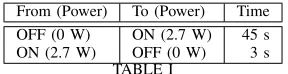
From (Power) To (Power) Time OFF (0 W) ON (2.7 W) 45 s ON (2.7 W) OFF (0 W) 3 s
TABLE I
TIME REQUIRED TO SWITCH FROM THEONSTATE TO THEOFFSTATE (AND VICE-VERSA)IN ALINKSYSWRT54GL.
In [3], authors demonstrate the feasibility and potential savings of RoD for 802.11 WLANs with “Survey, Evaluate, Adapt, and Repeat” (SEAR), a RoD framework based on heuristics that opportunistically powers on and off APs while maintaining coverage and user performance. In contrast to this experimental-driven approach, in [4] authors present the first analytical model for RoD, focusing on the case of “clusters” of APs (i.e., devices with overlapping coverage areas) and analyzing the impact of the strategy used to (de)activate on parameters such as the energy savings and the switch-off rate of the devices. In [5], authors extend the work of [4] to analyze the case when APs do not completely overlap their coverage areas, to understand the trade-offs when e.g. (re)associating clients from one AP to another AP in order to power down the former.
In both analytical works [4], [5], as well as in a recent follow-up analysis [9], among other simplifying assumptions, authors neglect the time required to power on an AP. However, in [3] it is reported that typical start-up times range between 12 and 35 seconds. To confirm these results, we perform an exper-imental characterization of the power consumed by a Linksys WRT54GL router running OpenWRT 10.03.1, which is a very popular wireless router that has been widely deployed, also measuring the average time required to power it on (i.e., the device starts broadcasting the SSID) and to power it off (i.e., no SSID is broadcasted). The results are provided in Table I. As our results confirm, these times are far from negligible, in particular when compared against inter-arrivals and/or service times. In this work we revisit this assumption and assess its impact on performance.
times. Our analysis is validated by extensive event-driven simulations, which confirm the validity of the model for a variety of scenarios.
Finally, in order to implement this vision, we propose and develop the OFTEN framework (Open Flow framework for Traffic Engineering in mobile Networks with energy aware-ness). We envision a centralised controller that (a)periodically performs TE optimisations based on a given set of policies. By using a common API for all technologies, this controller issues commands that are oblivious to the technologies underneath. Furthermore, the controller does not only serve to manage the mobile network infrastructure but can also reach mobile terminals and even trigger device-to-device communications between them. The goals of this work are aligned with some of the efforts currently being done at the Wireless and Mobile
Working Group of the ONF,1 where extensions to OpenFlow
for mobile network architectures are being studied.
To the best of our knowledge, this is the first attempt to implement a working prototype of OpenFlow that provides all these features and can be used in real networks. Indeed, while there have been several approaches proposed to manage heterogeneous mobile networks, they all suffer from one or more of the following limitations: ( ) they propose the general framework but do not fully specify and implement the un-derlying architecture [6]; ( ) they centralise the configuration but work at a much coarser time-scales [7]; and ( ) they do not seamlessly integrate different wireless technologies nor manage end-terminals in an integrated manner [8].
II. PERFORMANCEANALYSIS
Our system is a simplified version of the cluster model
analyzed in [4], consisting of two identical APs serving the same area. One of the APs is always on, in order to maintain the WLAN coverage, while the other AP is opportunistically powered on (off) as users arrive (leave) the system. However, in contrast to the model in [4], powering on the second AP
takes units of time; during this time, the second AP is
not available and arriving requests are served by the first AP.
Each AP consumes units of power h four users no AP
is deactivated. Only when the limit is reached, the
second AP is switched off and only one AP remains active.
This example corresponds to a hysteresis of .
We characterize the performance of the system with the following figures:
The average power consumed by the infrastructure
The average time spent in the system by a user .
The probability that a user is not allowed into the system
because of reaching the hard limit of users, i.e., the
blocking probability .
The rate at which the second AP is powered on/off , which is another key variable of interest as it can affect the lifetime of the equipment.
The focus of the work is first to model the impact of on these variables, then to understand the different trade-offs
1Open Networking Foundation: http://opennetworking.org/
two APs
A
B
C
Ton
Nh+1 Nl
one AP second AP
booting up
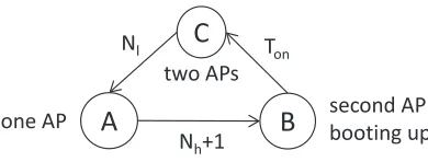
Fig. 2. Regenerative process to model the system.
in performance, and finally to derive the optimal configuration of an RoD scheme based on an optimization criterion.
A. Analytical model
We model our system with the regenerative process [13]
illustrated in Fig. 2. This regenerative process is formed by three stages, which depend on the status of the second AP:
Stage , in which the second AP is inactive.
Stage , in which it is being powered on but cannot serve clients yet.
Stage , in which both APs are active and serving users. Following the description of the system model, there are three transitions:
The transition , which is produced when there
are users associated with the first AP and a new user
arrives.
The transition , which is triggered by the
completion of the units of time required to power
on the second AP.
The transition , which occurs when there are
users in the system and one of them leaves.
We note that, in case there are or fewer users when the
transition happens (i.e., a number of users left while
the second AP was switching on), we will consider that the
system traverses state with a zero sojourn time, and then
transition to state .
In the following, we first describe how to compute the performance figures of the complete system, based on per-stage variables, and then present a model for the dynamics of the system, based on a Markov chain model for each stage. Throughout the article, we will refer with “stage” to the three states of the regenerative process illustrated in Fig. 2, and reserve the use of “state” for the description of the Markov chains. We note that this analysis of a two-AP scenario is exact as long as the assumptions on the arrival and departure processes, and the (re)association times hold.
B. Computing the overall performance figures
The average duration of a complete cycle of the
regen-erative process can be computed as
(1)
where is the average sojourn time of stage .
Note that, in our scenario, we have by definition that
, while the computation of and will be performed
4
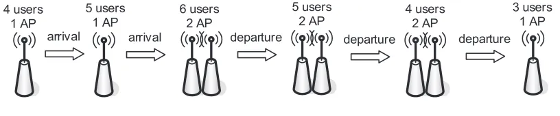
4 users1 AP
departure 3 users
1 AP departure
5 users 2 AP arrival
5 users
1 AP 6 users2 AP
arrival departure
4 users 2 AP
Fig. 1. Example of the powering on/off process for and .
Based on the , the average power consumed by the
network is
(2)
To compute the other performance figures, we need to obtain the expected amount of time that there are users in the system
during the duration of a cycle, . Similarly to (1), this value
can be expressed as
(3)
where is the average amount of time that there are users
in the system during the sojourn time of stage . With the
values of and , the probability that there are users in
the system is given by
(4)
Based on the , the blocking probability is equal to the
probability that there are users in the system, i.e.,
(5)
while the average time spent by a user in the system is
given by Little’s formula:
(6)
where corresponds to the average number of users in the
system, which is computed as
(7)
Finally, the derivation of the deactivation rate of the second
AP is almost immediate, given that it correspond to the
in-verse of a complete power on–power off cycle, i.e., the average duration of a cycle of the regenerative process. Therefore, it can be computed as
(8)
With the above, we can compute the performance figures of
the system with (2), (5), (6), and (8), given the times and
. We next describe how to compute these by modeling the dynamics of each stage of the regenerative process.
1 Nh+1 2K
0
…
…
µ µ µ µ µ
ʄ ʄ ʄ
ʄ ʄ
Nh Nh+1
0
µ µ
ʄ
ʄ ʄ
1
µ
ʄ
…
Nl Nl+1 2K
2µ 2µ 2µ
ʄ ʄ
2K-1
2µ
ʄ
…
(a) CTMCA
(b) CTMCB
(c) CTMCC
Fig. 3. CTMCs representing the different stages of the regenerative process.
C. Modeling each stage of the regenerative process
The three stages of the regenerative process can be mod-eled with three different Continuous-Time Markov Chains (CTMCs), illustrated in Fig. 3. In all the chains, the state models the number of users being served by the system, each chain having a different number of states:
CTMCAmodels the system when only one AP is powered
on, and therefore its number of states ranges from
(empty system) to (the system transitions to the
next stage).
CTMCB models the system during the units of time
it takes for the second AP to power, and therefore it can
serve between and the maximum number of users .
CTMCCmodels the system when the two APs are serving
users, and therefore ranges between and (the
system transitions to stage A).
We next analyze each of these CTMCs separately, starting
1) CTMCB: This case is illustrated in Fig. 3b, where users
arrive at a rate and are served at a rate . Our aim is to
compute the expected total time the CTMC spends in each
state during the interval . If we define as the
probability that a CTMC is in state at time , the expected
total time spent in that state during the interval is
d (9)
and based on this, we can compute , which
is required to derive the performance figures of the system as explained in the previous section.
To compute , we must solve the differential equation
d
d Q (10)
where andQare the vector of state probabilities and the
generator matrix of the CTMC, respectively.
For CTMCBwe have that
and
Q
with the elements of this matrix being
for and
for for and for
and for
and
in any other case
(11)
We also need the set of initial conditions to solve
(10). Given that stage starts when there are users in the
system and a new arrival happens, we have that for
in any other case
With these, we can solve the system specified by (10) and
compute with (9) as explained above.2 Note that we can
also obtain , which is required to compute the set of
initial conditions for both the next stage and stage , as
explained next.
2) CTMCC: This case is illustrated in Fig. 3c, with the
departure rate being as both APs are serving users. In
contrast to the previous chain, CTMCChas an absorbing state,
namely, . When the system reaches this number of users,
the second AP is powered off and the system transitions to stage .
As in the previous case, we need to compute the expected total time the chain spends in each state during the sojourn
2Instead of solving (10) and then computing (9), and can be efficiently evaluated for a given value using theuniformization
method.
time . These values correspond to thetime until absorption
spent in each of the non-absorbing states of CTMCC, which are
defined as for the set of states .
The times before absorption can be computed as [14]
(12) where
and
Q
with
for for and for
and for
and
in any other case
(13)
The initial conditions are determined by the
distri-bution of the state probabilities at the end of stage B, i.e.,
: if there are less than users in the system,
the second AP is immediately powered off and the system transitions to stage A; otherwise, the number of users at the end of stage B corresponds to the number of users at the beginning of stage C.
Following the above, we have that for
in any other case
Therefore, the system will spend zero sojourn time at stage
C with probability .
Once (12) is solved, the sojourn time of state can be
computed as
(14)
and for and 0
else-where.
3) CTMCA: This case, illustrated in Fig. 3a, is also modeled
with a CTMC with an absorbing state, namely, .
This state triggers the activation of the second AP, which corresponds to the transition to stage .
The times before absorption can be computed also with (12), where now we have
and
with
for and
for and for
and for
and
in any other case
(15)
Similarly to the case of CTMCC, the set of initial conditions
is determined by the status of the system at the end of
stage B: in case there were less than users once the second
AP is available, the system will transition directly to stage A, i.e.,
for (16)
otherwise, the transition to stage A will happen through state , i.e.,
for (17)
and correspondingly for any other state.
Finally, the sojourn time of state is computed as
(18)
and for and 0 elsewhere.
III. IMPACT OF ON PERFORMANCE
To analyze the impact of on the performance, we
assume a system in which up to users are allowed,
W, and arrivals/s and s, which
corresponds to an average load of approx. 50%.3We consider
four different activation policies:
: no hysteresis and the activation threshold lower than the maximum number of user per AP ( ).
: no hysteresis and the activation threshold
set to .
and : a hysteresis of two users and an
activation threshold set to .
and : a hysteresis of three users and an
activation threshold equal to .
When presenting the results, we depict with lines the values from our analytical model and with points the results of a discrete event simulator, where each point represents the average of ten simulation runs, each run consisting on more
than user departures (we do not represent the
95%-confidence intervals as their relative size is well below 1%).
3These service times can emulate a scenario where a user downloads e.g. 20 MB using 802.11g, assuming an effective throughput of approximately 15 Mbps.
22 24 26 28 30 32 34 36 38 40
0 5 10 15 20 25 30 35 40
Ts
(s)
Ton
Nh = 5, Nl = 5 Nh = 4, Nl = 4 Nh = 5, Nl = 2 Nh = 4, Nl = 2
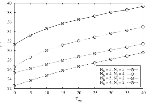
Fig. 4. Impact of the activation time on the total delay .
A. Total delay
We first analyze, for the four considered policies listed
above, the impact of on the total delay , with the
results shown in Fig. 4. There are several observations that can be drawn from the figure. First, the results from the model coincide with the simulations values for all consid-ered configurations (we obtained the same accuracy for other configurations of the load, omitted for space reasons), which confirms the validity of our analysis. Second, the results also
confirm that has a non-negligible impact on performance,
as it increases delay figures by 25–35% as compared to the case of zero start-up times. Finally, the policy more reluctant
to power on the second AP (i.e., ) results
in the largest delays for all values of , while the policy
more eager to power on the second AP (i.e., )
results in the smallest delay values.
B. Power consumed
We next analyze the impact of on the total power
consumed by the network with the four considered policies, with the results shown in Fig. 5. First, as in the previous case,
it is clear that has significant impact on the performance
w.r.t. this variable as well, as it increases power consumption by up to 20%. In addition to the above, which confirms the
quantitative impact of on performance, we note that
non-zero start-up times introduce qualitatively different results.
For instance, when , the less consuming scheme is
(as somehow expected, given the previous
results about the total delay ); however, when s,
the less consuming policy becomes . We
also note that the policy that resulted in the smallest delays
( ) has the largest power consumption only
for . More specifically, there is a trade-off between
delay performance and power consumption for , i.e.,
less consuming strategies lead to the largest delays; however,
when s, this trade-off disappears partially under some
3.8 4 4.2 4.4 4.6 4.8 5 5.2
0 10 20 30 40 50
Power (W)
Ton (s)
Nh = 5, Nl = 5
Nh = 4, Nl = 4 Nh = 5, Nl = 2
Nh = 4, Nl = 2
Fig. 5. Impact of the activation time on the power consumed .
0 0.005 0.01 0.015 0.02 0.025
0 5 10 15 20 25 30 35 40 pB
Ton(s) Nh = 5, Nl = 5
Nh = 4, Nl = 4
Nh = 5, Nl = 2
Nh = 4, Nl = 2
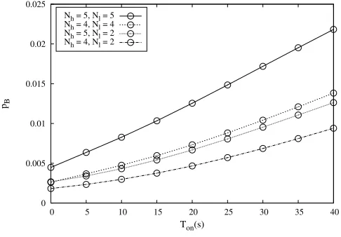
Fig. 6. Impact of the activation time on the blocking probability
next section). In this way, a strategy designed for can
be outperformed by other policies when (indeed, for
s it is outperformed by two strategies).
C. Blocking probability
Concerning the results on the probability that a user is
not allowed into the system, because the maximum capacity has been reached, they are presented in Fig. 6. The observed behavior in this case is somehow expected, given
the results on presented in Fig. 4, with the relative order of
the different activation policies being the same: the higher the delays (because the second AP is powered off for relatively longer periods of time), the higher the probability that a user cannot be admitted into the system.
D. Activation rate
Finally, we analyze the impact of on the rate at which
the second AP is powered on and off , with the results being illustrated in Fig. 7. As (somehow) expected, the results show that, in general, the longer it takes the AP to boot, the less
0 0.2 0.4 0.6 0.8 1 1.2
0 10 20 30 40 50 60
ω
(cycles/min)
Ton (s)
Nh = 5, Nl = 5 Nh = 4, Nl = 4 Nh = 5, Nl = 2 Nh = 4, Nl = 2
Fig. 7. Impact of the activation time on the activation rate
frequently it will go through the process of activation and deactivation. The figure also shows that those policies with
more hysteresis (i.e., ) are less sensitive to , the
reason being that the hysteresis increases the average sojourn
times of stages and , thus decreasing the influence of the
term in (8).
IV. ON THE TRADE-OFFS IN ARODSCHEME
Building on the previous results, in this section we analyze the different trade-offs that appear in a network that imple-ments a resource on demand scheme. More specifically, in the previous section we have seen that, depending on the
and configuration, and the value of , the performance
in terms of , , and changes both qualitatively and
qualitatively. Now we want to further explore these changes, considering also different values of the system load .
Throughout this section we will focus our findings on the most illustrative trade-offs, namely:
1) Total delay ( ) vs. power consumption ( ). This trade-off serves to represent the cost in terms of power consumption for a given gain in terms of performance, e.g., how many watts costs a given reduction in seconds. 2) Power consumption ( ) vs. activation rate ( ). This trade-off illustrates that the resource consumption has two dimensions that must be carefully considered when configuring the RoD scheme, since a decrease of the power consumption may lead to an undesirable increase
of the activation rate of the second AP.4
A. Impact of
We start our analysis with the impact of on the two
considered trade-offs. To this aim, we build on the results
from the previous section (i.e., ), and depict them in
Figs. 8 and 9, where each point corresponds to a pair of values
20 25 30 35 40 45
3.5 4 4.5 5 5.5
Ts
(s)
Power (W) Nh = 5, Nl = 5
Nh = 4, Nl = 4 Nh = 5, Nl = 2 Nh = 4, Nl = 2
Ton = 0
Ton = 60
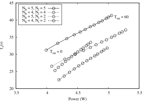
Fig. 8. Impact of the activation time on the vs. trade-off.
2 3 4 5 6 7 8
0 0.2 0.4 0.6 0.8 1 1.2
Power (W)
ω (cycles/min)
Nh = 5, Nl = 5
Nh = 4, Nl = 4
Nh = 5, Nl = 2
Nh = 4, Nl = 2
Ton = 0
Ton = 60
Fig. 9. Impact of the activation time on the vs. trade-off.
( for Fig. 8, and for Fig. 9) for a different value
of .5
On the one hand, Fig. 8 illustrates that, as already showed
in the previous section, the longer the value of , the worse
the performance of the system both in terms of and ,
and that different configurations result in different
performance figures, both quantitatively and qualitatively. The
figure also shows another effect of non-zero , namely, that
there are some configurations worse than others under all
circumstances. Indeed, while for the case of , if one
configuration results in a lower delay than other it also results in a larger power consumption, this is no longer true when
. For instance, when s, the configurations
and obtain worse figures ofboth
and than the other two configurations.
On the other hand, Fig. 9 reveals one “positive” aspect of
a longer : given that it takes longer to complete a cycle of
the regenerative model, the power consumption increases but
5Given the tight matching between analytical and simulation values, from now we will only represent the values corresponding to the analysis.
5 10 15 20 25 30 35 40 45 50
3 3.5 4 4.5 5 5.5 6 6.5 7
Ts
(s)
Power (W)
Nh = 5, Nl = 5 Nh = 4, Nl = 4
Nh = 5, Nl = 2 Nh = 4, Nl = 2 ρ = 0.05
ρ = 0.95
Fig. 10. Impact of the load on the vs. trade-off.
the activation rate decreases, which could help to extend the
lifetime of the second AP.6
B. Impact of
We next analyze how the trade-offs varies for different
values of the network load . To this aim, we set equal to
30 s and plot the two considered trade-offs for values ranging between 0.05 and 0.95 in steps of 0.05, with the results being
depicted in Figs. 10 and 11. For the case of the vs.
trade-off (Fig. 10), we can derive the following main results: When the load is very low, there is very little difference between the (de)activation policies, as only one AP is on almost all the time.
When the load is very high, though, there are non-negligible differences in terms of power (approx. 4%) and, in particular, delay (approx. 30%) between the best and worst performing case. In all cases, the power consumption is very close to 7 W, hinting that the second AP is on most of the time, either booting (stage B) or activated (stage C). The difference in delay performance
depends on the value of : the smaller this value, the
longer the system stays in stage C, thus providing users with better service.
Like for the case of , seen in the previous section,
there are qualitatively variations in the vs. trade-off
when changes, as the lines corresponding to different
configurations not only change their slope but also might cross each other.
Given a value, a configuration without hysteresis
( ) obtains a poorer performance both in terms
of and than the configuration with hysteresis
( ) forallthe values of .
We next analyze how the vs. trade-off varies with
, which is illustrated in Fig. 11 and shows a very-different behavior as compared with the case of the variation with
2 3 4 5 6 7 8
0 0.1 0.2 0.3 0.4 0.5 0.6 0.7 0.8 0.9
Power (W)
ω (cycles/min)
Nh = 5, Nl = 5 Nh = 4, Nl = 4 Nh = 5, Nl = 2 Nh = 4, Nl = 2
ρ = 0.95
ρ = 0.05
Fig. 11. Impact of the load on the vs. trade-off.
. Based on the figure, we can derive the following main conclusions:
Again, for small values, there are little differences
between configurations, with being very close to the
use of only one AP and being close to 0.
As increases, performance worsens for both variables,
i.e., there is an increase of the power consumption and the activation rate, the former already seen in the previous figure, while the later being caused by the crossing of the
threshold due to the larger load.
However, once a certain threshold is crossed, power
consumption keeps increasing but the activation rate decreases: this is because, the higher the load, the less
likely the threshold will be reached, and therefore the
system will increase the amount of time with both APs active, which results in a smaller .
Like in the previous case, strategies without hysteresis obtain worse figures than those with hysteresis, since the total power is similar for both types of RoD schemes but the activation rate is much higher when no hysteresis is employed.
V. OPTIMAL CONFIGURATION OF ARODSCHEME
Our model not only serves to analyze the trade-offs in a WLAN implementing a RoD scheme, but also can be used to derive the optimal configuration of its parameters (namely,
and ) for a given scenario (in terms of and ), as we
illustrate next. We note that there are many different algorithms and configuration criteria that could be used to configure the WLAN, and therefore that our proposal only serves to illustrate one approach.
A. Optimization Algorithm
Our optimization criterion is as follows. For our 2-AP setting, the best performance in terms of delay for any value is the one provided when both APs are always active.
We denote this minimum average delay as . Then, we
assume that the network administrator is willing to trade-off
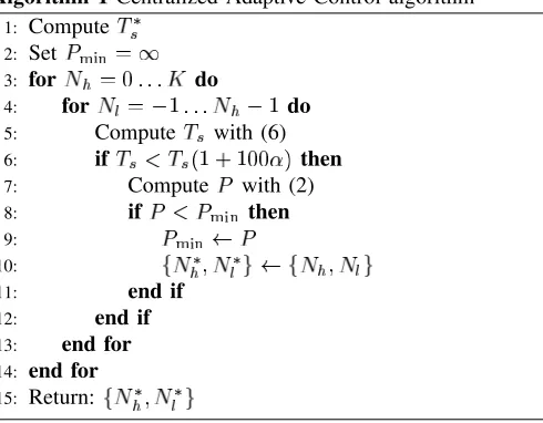
Algorithm 1 Centralized Adaptive Control algorithm
1: Compute
2: Set
3: for do
4: for do
5: Compute with (6)
6: if then
7: Compute with (2)
8: if then
9: 10:
11: end if 12: end if 13: end for 14: end for
15: Return:
an increase of this average delay by e.g. % in exchange
for a better power consumption by means of a RoD scheme.
To this aim, we sweep on all possible values of and
, and select that configuration with the minimum power
consumption (denoted as ) among all the ones with an
average delay smaller than . We denote this
configuration as .
We sumarize the operation of this scheme in Algorithm 1, whose computational complexity is relatively small (i.e., it consists on two sweeps over a small number of possible con-figurations). We note that the sweep includes the configuration
with and , i.e., the case of the two APs
always on, and therefore the algorithm will always provide at least this configuration as a result.
B. Results
Fig. 12 shows the optimal configuration for (top)
and s (bottom). In both cases, when the load is low
( ), the most efficient strategy is to use large values
of and , since the probability that the system reaches a
high number of users is very small. These values are almost the same when there is no start-up time and when it is
s. As the load increases, the values of and decrease
to ensure that the total delay does not exceeds the imposed
threshold. In this case, when is 30 s, higher values of
hysteresis (and therefore lower values of ) are required to
decrease the activation rate of the system and minimize the
time spent in stage B. Additionally, the value of is also
lower to ensure that not many users are in the system when the second AP is being powered on.
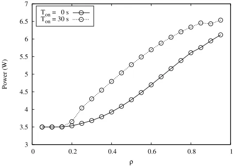
If we compare the power consumption of the optimal
strategies for and s (Fig. 13), we can
see that this is identical when (since the values of
and are almost the same in both cases). For , the
power consumption when s is always higher due to
the use of lower values of and that increases the time
0 1 2 3 4 5 6
0 0.2 0.4 0.6 0.8 1
Ton = 0 s
N
Nh Nl
0 1 2 3 4 5 6
0 0.2 0.4 0.6 0.8 1
Ton = 30 s
ρ
Fig. 12. Optimal configuration of and vs. with and s.
3 3.5 4 4.5 5 5.5 6 6.5 7
0 0.2 0.4 0.6 0.8 1
Power (W)
ρ
Ton = 0 s
Ton = 30 s
Fig. 13. Power consumption with , and .
VI. AN ARCHITECTURE FORRODSCHEME
In this section, we introduce the OFTEN framework (Open Flow framework for Traffic Engineering in mobile Networks with energy awareness). Our approach is based-on a cen-tralised controller that (a)periodically performs TE optimisa-tions based on a given set of policies. By using a common API for all technologies, this controller issues commands that are oblivious to the technologies underneath. Furthermore, the controller does not only serve to manage the mobile network infrastructure but can also reach mobile terminals and even trigger device-to-device communications between them.
A. Architectural elements
We propose the architecture illustrated in Fig. 14, which consists of a number of technology-agnostic elements plus some technology-specific modules. We start with the former: The first element is the database containing the current
network vision, i.e., thenodesof the network, the active
linksconnecting them, the potential links that can be used and their capacity as well as the traffic demand.
Based on this network vision, theoptimisermodule runs
(a)periodically (e.g., every 5 minutes or after a major change in network conditions) to obtain the configuration that maximises performance, according to a set of given policies that trade-off energy consumption and perfor-mance.
The configuration resulting from the optimiser module
is passed to thecontrollervia thenorthboundinterface;
this interface is not shown in Fig. 14 and depends on the specific OpenFlow controller chosen (we leave it outside the scope of our architecture).
Finally, the controller implements this configuration
through OpenFlow++, a technology-agnostic interface
that extends the OpenFlow protocol (OFPT) to support the required functionality for mobile networks (described in the following sections).
One key feature of the proposed architecture is the ability of the upper layer modules described above to operate on a technology-agnostic manner, which allows to ( ) manage the entire heterogenous network in an integrated way, allowing for a joint optimisation of all the technologies; and ( ) easily adapt network operation to new requirements/objectives, by simply modifying the technology-agnostic modules. This functionality is enabled by the following lower layer modules, which are technology-specific:
A technology dispatcher, which is responsible to re-direct the OpenFlow++ primitives to appropriate technology-specific module.
Technology-specific mapping modules, which convert
the OpenFlow primitives into the primitives of the cor-responding technology and viceversa; among others, this includes the setting of new configurations and update the network vision.
Another key feature is that the architecture can be ex-tended to support new technologies in a non-disruptive way: to enable the use of a new technology, we only need to design the specific mapping module and a minor extension to the Dispatcher to identify when a command is from/to that specific technology. We note that, because of this centralised management of all technologies in the network, the controller might suffer from scalability issues, a general concern in SDN scenarios. To ease this burden, one possible solution would be the definition of hierarchical areas [17], [18].
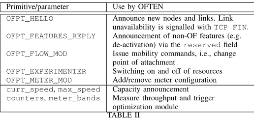
We next describe the technology-agnostic operation of the upper modules and how the OpenFlow++ interface is used and extended to support this vision (we summarise in Table II the required extensions to OpenFlow), while the technology-specific operation is described in the next section.
OpenFlow ++
802.11 Network
vision
LTE D2D
Controller
Optimiser agnostic Technology
802.11 LTE D2D
Technology
specific
Policies
OFPT
Technology dispatcher Mapping modules
Fig. 14. Open Flow-based SDN architecture for heterogeneous networks.
Primitive/parameter Use by OFTEN
OFPT_HELLO Announce new nodes and links. Link unavailability is signalled withTCP FIN.
OFPT_FEATURES_REPLY Announcement of non-OF features (e.g. de-activation) via thereservedfield
OFPT_FLOW_MOD Issue mobility commands, i.e., change point of attachment
OFPT_EXPERIMENTER Switching on and off of resources
OFPT_METER_MOD Add/remove meter configuration
curr_speed,max_speed Capacity announcement
counters,meter_bands Measure throughput and trigger optimization module
TABLE II
EXTENSIONS TOOPENFLOW INTRODUCED BYOFTEN.
map the actual physical network, like e.g. the one illustrated in Fig. 15 (top), into an abstract vision (bottom). While the physical network is composed of wired links in the backhaul, relatively stable links from mobile terminals to cell towers, higher capacity but more dynamic connections to 802.11 Access Points, potential device-to-device links, etc., in the abstract vision there are nodes and links, each with a different capacity, that can be reconfigured and switched on and off as required by the optimiser.
The proposed architecture is flexible to accommodate differ-ent TE mechanisms for the optimiser, depending on the com-putational resources availability, complexity of the network, and periodicity/timeliness of the operation of the optimisation (see Section IV.C for a description of the mechanism used in our implementation). Furthermore, the optimisation of the net-work does not have to be changed whenever a new technology is introduced, and only requires mapping the features of the
new technology to our abstractions.7
The mapping between the actual network and the abstract one is made in the technology dispatcher module, which performs the association between the mapping modules and the OpenFlow++ interface. This interface is the central element of the architecture that supports the following functionality with technology-independent primitives: ( ) the maintenance
7Of course, to achieve this it is critical that our abstraction is general enough to cover the functionality provided by the new technology, as otherwise the optimiser would need to be adapted to the novel functionality provided.
LTE Physical Network
Controller vision
Fig. 15. Physical network (top) and abstract vision (bottom). Grey circles denote nodes in power-saving mode, dotted lines represent available links, and solid lines represent used links.
of the information in the database, including changes to link capacities, reachability, etc., ( ) the control of the forwarding tables, and ( ) the (de)activation of resources. We next describe the OpenFlow commands upon which we rely, as well as the extensions required, to support these features.
2) Maintaining the network vision: The first challenge is to maintain the list of nodes that compose the network, which in our case appear and disappear more frequently than in “traditional” (wired) networks, due to users’ mobility and wireless propagation. For the case of nodes connected to the network, i.e., APs or eNBs, they just have to establish a
connection to the default OpenFlow transport protocol 6653
via TLS or TCP, and then perform the usual OFPT_HELLO
exchange. For those nodes that can be (de)activated, we need to extend the database to announce this feature, which we do
via the reserved field in the OFPT_FEATURES_REPLY
message.
For the case of nodes that are one or more hops away from the wired infrastructure, we do not require them to implement any (major) modification and, in particular, to support OpenFlow. However, as they have to appear as nodes in our vision, we require that the PoAs act on the behalf of the terminals, and register them with the controller (following the standard procedure) whenever they detect there is a new node or a new candidate link. When no link towards a terminal is
available, the connection is terminated via e.g. a TCP FIN
message. Thus, in order to keep the list of nodes available in the network, our architecture does not need to introduce changes to the OpenFlow specification, but only to ensure that the database of (de)registered nodes is updated when required. Similarly, in order to announce the capacity of the links that connect two or more nodes, we can rely on the struc-tures already defined by the OpenFlow specification, i.e., the
e.g. WLAN interference, a node moves away from the eNB), the node responsible for a link needs to modify the value of the corresponding parameters.
Finally, the usage of the links carrying data can be easily
tracked with per-flow counters. By periodically polling
these counters with read operations, the database can identify which links are becoming congested and which ones are being under-occupied and could support more traffic. This can then trigger the corresponding optimisation. We note that an alternative implementation could be based on the use of per-flowmeters; indeed, by specifyingmeter bands, we can trigger an action when certain thresholds are passed.
3) Installing a new configuration: For wired links, the set-ting of forwarding paths does not require to modify the default OpenFlow operation. With our abstraction, a wireless terminal can be considered as a node with a number of ports but only one active forwarding entry at a time, which corresponds to the selected point of attachment. In this way, changing the point of attachment only requires modifying a flow entry via the OFPT_FLOW_MODmessage, e.g. to change of the Access Point the node is associated with, or the use of the cellular link. As we describe next, the Technology Dispatcher decides the technology specific module that handles the commands and triggers the protocol-specific operations to implement the change. As in the previous case, there is not need to specify new OpenFlow primitives.
4) Switching on/off resources: Energy-efficient operation of a network requires the ability to power on and off resources as required [19]. Accordingly, our architecture has been de-signed to provide such support. For the corresponding set of operations, we cannot rely on or extend the default OpenFlow primitives, and therefore we need to specify new primitives. To do this, we rely on the “experimenter” symmetric messages (OFPT_EXPERIMENTER), which are used for those nodes that upon registration announced that they supported deactiva-tion, in addition to the time it takes to switch between states (so the the controller can preemptively activate resources) and the corresponding power consumption (to duly optimase energy consumption).
Following the above, we extend the OpenFlow set of
primitives with a pair of commands, switch_on and
switch_off, to power on and off (respectively) a given node. As we will describe in our testbed, these primitives can be used even when nodes do not support a sleep state, but are connected to e.g. a switched rack power distribution units (PDU), which can be remotely controlled via a network connection.
B. Mapping to technologies
The architecture enables an integrated traffic management of a heterogeneous mobile network, through the use of the Open-Flow++ primitives. We next describe how these primitives are mapped back-and-forth into technology-specific functionality thanks to the technology dispatcher, which acts as a relay of the messages between the OpenFlow++ API and the modules
doing the mapping.In nuce, we require the ability to:
Detect when new nodes and links are available, including the potential points of attachment to the network. Estimate the available capacity of the wireless links. Change the point of attachment of a terminal without disrupting the traffic served.
In what follows, we describe how the above is supported by the dispatcher and the current wireless technologies, by just introducing minor extensions to their operation.
1) Technology dispatcher: New nodes or available links are announced in a technology-specific manner to this module (as detailed next), which then performs the translation to the OpenFlow++ API. With this module, a mobile terminal detected by a set of access points and an eNB (i.e., multiple announcements) is registered only once as a node, but with a set of candidate links towards existing nodes. Given that wired nodes may support different deactivation techniques (e.g., wake-on-LAN, switched power distribution units), this module needs to be aware of the specific technique supported in order to issue the corresponding commands when needed. The capacity of the wireless links is computed by each technology as described next, and then passed via the OpenFlow++ API using the parameters described above.
Changing the default forwarding table of a terminal corre-sponds to performing a handover, which can be intra- or inter-technology. The former is handled within each technology using its own mechanisms, while for the latter we rely on the 3GPP support for multiple radio access networks (RANs), including those that are non-cellular. The mobile 3GPP archi-tecture centralises the support of inter-RAN handovers on the cellular network (more specifically, on a set of network entities that may act as control and data plane anchors for the different handover scenarios). This is based on the assumption of full cellular coverage.
2) 802.11 mapping: In Wi-Fi networks there are at least three mechanisms to detect when a link towards a mobile
terminal is available: ( ) the probe request messages
the mobile periodically sends on different channels to detect known or new Access Points (APs), which can also trigger the presence of a new node that is duly reported to the technology dispatcher; ( ) passive scanning mechanisms; and
( ) theNeighbour Report message exchange from the
recent 802.11k amendment, already supported by new devices such as e.g. iPhones, which is used by mobile terminals to learn about APs in the surroundings, and by APs to gather measurements about the quality of the channel towards other APs, which are then reported to the network.
The estimation of the capacity of a link is supported by these measurements, building on e.g. the usual mappings of signal quality to maximum throughput, which are reported to the network vision database. In case a group of nodes contend in a WLAN, the AP can derive the achievable capacity thanks
to the use of thelinearised capacitymodel proposed in [20],
access into a simple linear-based model.8
Changing the point of attachment of a Wi-Fi node while providing a seamless experience results is very challenging, given that in 802.11 ( ) the mobile terminal typically selects its “best” point of attachment, and ( ) the signalling for carrier-grade operation is relatively complex. Still, thanks to the recent 802.11v and 802.11r amendments, this can be achieved with minor disruption of the service (this is validated by our prototype of Section VII). Fig. 16 illustrates a simplified version of the signalling occurring on the access network. Next, we describe how these interactions support the changing of the point of attachment when triggered by the OpenFlow command.
Following Fig. 16, when a terminal powers on, it authenti-cates and associates with the best AP (i.e., AP1), and performs the Neighbour Report exchange to learn about the APs in the vicinity belonging to the same network. During these operations, the APs that overhear the node activity report on the different links available to the mobile terminal, and update the database accordingly (among these, AP2 in the Figure). Assuming at some point that the optimiser decides that it
is better if the mobile node (MN) associates with AP2, the
controller issues aOFPT_FLOW_MODprimitive to change the
(only) default forwarding entry ofMN, from nodeAP1to node
AP2. This primitive is processed by the 802.11 module with
the controller, which issues a command to AP1 to trigger the
802.11vBSS Transition Requestmessage, so the MN
associates with AP2. Thanks to the use of 802.11r, this re-association is noticeably shorter than the original one. As we will see in the next section, the controller can duly issue other OpenFlow primitives to minimise the impact on performance.
3) Cellular mapping: We next describe the guidelines to implement a technology-specific module similar to the one described above for the case of cellular networks. While 3GPP-based networks involve more complex procedures, they also tend to favor a centralised control and estimation of resources, and therefore we expect that the design of this module is simpler than in the Wi-Fi case. However, given that cellular networks are designed for large deployments, one key difference with Wi-Fi is on maintaining user location.
If we focus on packet switched communications in a cellular network the list of active users within a cell is available at the Mobility Management Entity (MME), while the inactive users are less accurately located.
The above challenges the implementation of infrastructure-on-demand schemes, as a group of inactive users could sud-denly change to be active in a certain geographical area, and an aggressive energy-saving policy might have powered off too many Base Stations to promptly react to the demand. Except for this, cellular networks readily provide the means to support the requirements of the extended OpenFlow interface: active UEs periodically report the quality of the channel
8Note that the proposed linearised capacity model can also be used to abstract the capacity of any technology, including OFDM, CDMA, etc.
towards other Base Stations, and network-initiated handovers are supported.
4) Device to device mapping: Our architecture also sup-ports device-to-device communications, where mobile nodes opportunistically share wireless links for a better performance. However, in contrast to the previous cases, this paradigm requires introducing modifications to the mobile terminals. To that aim, we have adapted our SOLOR framework [21], which builds on Wi-Fi Direct to opportunistically create D2D groups, to communicate with the technology dispatcher to announce link availability and support the set-up and release of this links. Given that SOLOR is a decentralised mechanism, the adaptation consists basically on centralising the control of the modules.
VII. PROOF OF CONCEPT
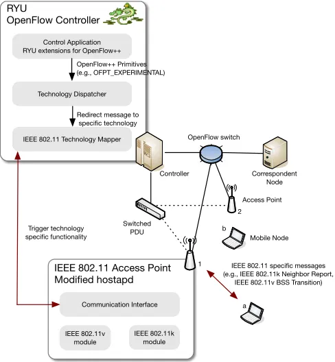
To validate the feasibility of our approach, we have pro-totyped our architecture in a small testbed that includes the technology specific modules for Wi-Fi. The testbed, deployed in an office setting, is depicted in Fig. 17 and consists of one controller, an OpenFlow switch, two APs, two MNs, a correspondent node (CN) to support traffic generation, and a switched PDU to support the (de)activation of APs via HTTP requests.
OpenFlow switch
Switched PDU
Controller Correspondent Node
Access Point
Mobile Node
1 2
a b RYU
OpenFlow Controller
Control Application RYU extensions for OpenFlow++
Technology Dispatcher
IEEE 802.11 Technology Mapper OpenFlow++ Primitives (e.g., OFPT_EXPERIMENTAL)
Redirect message to specific technology
IEEE 802.11 Access Point Modified hostapd
Communication Interface
IEEE 802.11v module
IEEE 802.11k module Trigger technology
specific functionality
IEEE 802.11 specific messages (e.g., IEEE 802.11k Neighbor Report,
IEEE 802.11v BSS Transition)
Fig. 17. Deployed testbed and implemented modules and interfaces.
A. Implementing seamless NIHO
Authentication Authentication Association request Assocation response
IEEE 802.1x/RADIUS Signaling
BSS Transition Request (to AP2) BSS Transition Response
Reassociation request (Fast BSS transition) Neighbor Report Request
Neighbor Report Response
Data exchange Data exchange
...
IEEE802.11k
IEEE 802.11v
IEEE 802.11r
The controller knows the MN is associated to AP1
OFPT_EXP. (Get list of APs) Trigger IEEE 802.11k Neighbor Report Request
Return IEEE 802.11k Neighbor Report Response Information
OFPT_FLOW_MOD (change MN PoA) Trigger IEEE 802.11v BSS Transition Request to AP2
Confirmation of Handover
OFPT_FLOW_MOD (response) OFPT_EXP. (Get list of APs) Technology
Dispatcher IEEE 802.11
Mapper Controller
Technology specific Technology agnostic
RADIUS AP2
Reassociation response (Fast BSS transition) AP1
MN/STA
Fig. 16. Simplified handover operation.
change the point of attachment of a MN: (1) activate at the
switch bicastingof traffic between the CN port and the ports
the APs are connected to; (2) issue the 802.11v BSS Tran-sition Request; (3) wait until the handover is completed, and inform the controller accordingly; and (4) stop the bicasting of traffic at the switch and re-configure the forwarding tables accordingly.
B. Software setup
The controller is a desktop machine running Linux and
the Ryu SDN framework,9 which we extend to support the
proposedOpenFlow++API, and two Python libraries: one to
map theswitch_on/offcommands to the switched PDU,
and another one for the 802.11-specific mechanisms. The
controller also runs a MySQLdatabase10 to keep the network
status. Our controller uses a variation of the TE algorithm that we designed in Section V-A, using the configuration
and . Other TE schemes could be supported, based
on, e.g., flow management policies or traffic measurement requirements (see [22] for a recent survey).
The APs are small PCs running Linux and extended to sup-port the required functionality as follows. We have modified
the widely used hostapd demon11 to set up a connection
with the 802.11 module at the controller, so that the AP can report changes in the network conditions (which are updated to the database) and can set up new configurations. When the
9http://osrg.github.io/ryu/ 10http://www.mysql.com 11http://w1.fi/hostapd/
controller issues a change on the default forwarding path of a node, the 802.11 module translates this primitive to an 802.11k request to perform channel measurements (so that the mobile updates the list of available APs) and an 802.11v command to change the point of attachment. An overview of the developed software modules and interfaces is depicted in Fig. 17.
The CN is a regular desktop machine, while the MNs
are small PCs, like the switch, which runs OpenVSwitch.
Finally, we set up an additional desktop machine, not shown
in the picture, running the FreeRADIUS server12 to enable
the use of WPA2-enterprise as required by Wi-Fi Passpoint.
C. Supporting infrastructure on demand
To validate that the controller activates resources as traffic requirements vary, we perform the following experiment. We first generate a TCP flow between the CN and node , which
is associated with AP , while AP is inactive. At s,
we generate another TCP flow between the CN and node , which saturates the capacity of the link. Thanks to periodic measurements, the controller decides that more resources are
required, and switches on AP 2 since threshold has been
reached. Once this AP is available, it notifies the controller, which then immediately issues a handover trigger to node
that associates with the new AP at s.
D. Experimental validation
The results of this experiment are depicted in Fig. 18, where we plot the per-flow throughput (bottom) and the total
put (top) as measured by the Wireshark tool. According to the figure, the first TCP flow achieves at first about 20 Mbps, but when the second flow appears, its throughput its reduced to 5 Mbps, while the former gets about 15 Mbps (with some variations due to contention). Once this has been moved to AP 2, the flow from node gets again about 20 Mbps, while the flow from node gets about 20 Mbps as well.
0 5 10 15 20 25 30 35 40 45
0 10 20 30 40 50 60 70
0 1 2 3 4 5 6 7 8 9 Throughput (Mb/s) Power (W) Total Throughput Total Power 0 5 10 15 20 25 30 35 40 45
0 10 20 30 40 50 60 70
Time (s)
MN1 MN2
Fig. 18. Validation of the proof of concept.
We also represent in Fig. 18 the estimated energy consump-tion of the infrastructure, following the model of [23]. As compared with the case of both APs on, our solution reduces energy consumption by 18%, an improvement that comes at the cost of an increased delay, mainly because the time it takes to power-up the AP. Following the results reported in [19], we estimate that our framework could reduce energy consumption by 30–40% in a campus-wide deployment (note that our experiment corresponds to an “upper bound” in terms of performance reduction, as there is always wireless activity).
VIII. CONCLUSIONS
In this work we have presented an analytical model for the case of a simple RoD system, which takes into account the time required to power on an AP. The accuracy of the model has been validated via simulations, and results have showed that, even for the simple scenario considered, the time required to start-up an AP has a dramatic impact on performance. Indeed, this time alters both the quantitative and qualitative results as compared to the case of zero start-up time. We have also obtained the optimal configuration of a simple RoD scheme taking into account the start-up time, finding that this time modifies the optimal parameters of the RoD system. As a consequence, we believe that the start-up time should be taken into account when designing infrastructure on demand policies in real-life deployments.
We have also proposed a novel SDN architecture to support traffic engineering in mobile networks. Our OpenFlow-based architecture facilitates the support for heterogeneous tech-nologies by making use of abstractions, and enables the use of infrastructure-on-demand schemes via novel primitives to
switch on/off devices as required. The validity of our approach has been demonstrated for the case of 802.11 through a simple prototype.
REFERENCES
[1] W. Sun, O. Lee, Y. Shin, S. Kim, C. Yang, H. Kim, and S. Choi, “Wi-Fi Could Be Much More,”Communications Magazine, IEEE, vol. 52, no. 11, pp. 22–28, November 2014.
[2] P. Serrano, A. de la Oliva, P. Patras, V. Mancuso, and A. Banchs, “Green-ing wireless communications: Status and future directions,” Computer Communications, vol. 35, no. 14, pp. 1651 – 1661, 2012.
[3] A. Jardosh, K. Papagiannaki, E. Belding, K. Almeroth, G. Iannaccone, and B. Vinnakota, “Green WLANs: On-demand WLAN infrastructures,”
Mobile Networks and Applications, vol. 14, no. 6, pp. 798–814, 2009. [4] M. A. Marsan, L. Chiaraviglio, D. Ciullo, and M. Meo, “A simple
analytical model for the energy-efficient activation of access points in dense wlans,” inProceedings of e-Energy ’10. New York, NY, USA: ACM, 2010, pp. 159–168.
[5] A. P. C. da Silva, M. Meo, and M. A. Marsan, “Energy-performance trade-off in dense wlans: A queuing study,”Computer Networks, vol. 56, no. 10, pp. 2522 – 2537, 2012.
[6] C. Bernardos, A. de la Oliva, P. Serrano, A. Banchs, L. Contreras, H. Jin, and J. Zuniga, “An architecture for software defined wireless networking,”Wireless Communications, IEEE, vol. 21, no. 3, pp. 52– 61, June 2014.
[7] Y. Yiakoumis, M. Bansal, A. Covington, J. van Reijendam, S. Katti, and N. McKeown, “BeHop: A Testbed for Dense WiFi Networks,” in Proceedings of the 9th ACM International Workshop on Wireless Network Testbeds, Experimental Evaluation and Characterization, ser. WiNTECH ’14. New York, NY, USA: ACM, 2014, pp. 1–8. [8] L. Suresh, J. Schulz-Zander, R. Merz, A. Feldmann, and T. Vazao,
“Towards Programmable Enterprise WLANS with Odin,” inProceedings of the First Workshop on Hot Topics in Software Defined Networks, ser. HotSDN ’12. New York, NY, USA: ACM, 2012, pp. 115–120. [9] M. A. Marsan and M. Meo, “Queueing systems to study the energy
consumption of a campus WLAN,” Computer Networks, vol. 66, pp. 82–93, 2014.
[10] P. Serrano, A. Garcia-Saavedra, G. Bianchi, A. Banchs, and A. Azcorra, “Per-frame energy consumption in 802.11 devices and its implication on modeling and design,”Networking, IEEE/ACM Transactions on, vol. PP, no. 99, pp. 1–1, 2014.
[11] M. Papadopouli, H. Shen, and M. Spanakis, “Modeling client arrivals at access points in wireless campus-wide networks,” in Local and Metropolitan Area Networks, 2005. LANMAN 2005. The 14th IEEE Workshop on, 2005, pp. 6 pp.–6.
[12] G. R. Hiertz, D. Denteneer, L. Stibor, Y. Zang, X. P. Costa, and B. Walke, “The IEEE 802.11 Universe,”Comm. Mag., vol. 48, no. 1, pp. 62–70, Jan. 2010.
[13] J. Medhi,Stochastic Models in Queueing Theory. Academic Press, 2002.
[14] G. Bolch, S. Greiner, H. de Meer, and K. S. Trivedi,Queueing Networks and Markov Chains. Wiley-Interscience, 2006.
[15] Cisco, “Cisco Visual Networking Index: Forecast and Methodology, 2013-2018,” Cisco, Tech. Rep., june 2014. [Online]. Available: http://www.cisco.com/en/US/solutions/collateral/ ns341/ns525/ns537/ns705/ns827/white paper c11-481360.pdf [16] N. McKeown, T. Anderson, H. Balakrishnan, G. Parulkar, L. Peterson,
J. Rexford, S. Shenker, and J. Turner, “OpenFlow: Enabling Innovation in Campus Networks,” SIGCOMM Comput. Commun. Rev., vol. 38, no. 2, pp. 69–74, Mar. 2008.
[17] X. Li, P. Djukic, and H. Zhang, “Zoning for hierarchical network optimization in software defined networks,” inNetwork Operations and Management Symposium (NOMS), 2014 IEEE, May 2014, pp. 1–8. [18] X. Li and H. Zhang, “Creating logical zones for hierarchical traffic
engineering optimization in sdn-empowered 5g,” inProceedings of the International Conference on Computing, Networking and Communica-tion (ICNC), 2015, 2015.
[20] A. De La Oliva, A. Banchs, and P. Serrano, “Throughput and energy-aware routing for 802.11 based mesh networks,”Comput. Commun., vol. 35, no. 12, pp. 1433–1446, Jul. 2012.
[21] A. Garcia-Saavedra, B. Rengarajan, P. Serrano, D. Camps-Mur, and X. Costa-Perez, “SOLOR: Self-Optimizing WLANs With Legacy-Compatible Opportunistic Relays,” Networking, IEEE/ACM Transac-tions on, vol. PP, no. 99, pp. 1–1, 2014.
[22] I. F. Akyildiz, A. Lee, P. Wang, M. Luo, and W. Chou, “A roadmap for traffic engineering in sdn-openflow networks,”Computer Networks, vol. 71, no. 0, pp. 1 – 30, 2014.