Type of the Paper (Article)
ARIMA-M: A New Model for Daily Water
Consumption Prediction, Based on the
Autoregressive Integrated Moving Average Model
and the Markov Chain Error Correction
Hongyan Du 1,*, Zhihua Zhao 2, Huifeng Xue 3
1 China Aerospace Academy of System Scientific and Engineering, Beijing, China; [email protected] 2 Xi'an University of Technology, Xi’an, China; [email protected]
3 China Aerospace Academy of System Scientific and Engineering, Beijing, China; [email protected] * Correspondence: [email protected];
Abstract: Water resource is considered as a significant factor in development of regional environment and society. Water consumption prediction can provide important decision basis for the regional water supply scheduling optimisations. According to the periodicity and randomness nature of the daily water consumption data, a Markov modified autoregressive moving average (ARIMA) model is proposed in this study. The proposed model, combined with the Markov chain, can correct the prediction error, reduce the continuous superposition of prediction error, and improve the prediction accuracy of future daily water consumption data. The daily water consumption data of different monitoring points are used to verify the effectiveness of the model, and the future water consumption is predicted, in the study area. The results show that the proposed algorithm can effectively reduce the prediction error compared to the ARIMA.
Keywords: water resource management; water consumption prediction; Markov chain; autoregressive moving average model; error correction
1. Introduction
Water resources are considered as an important key factor for regional sustainable development, in both developing and developed countries. With the development of urbanization and the improvement of people's living standard, the demand for water supply is increasing, and the shortage of water resources is becoming more and more serious. A crisis of water scarcity occurs in many parts of the world. With the expansion of the scope and scale of the urban water supply system, the complexity of the water supply has been significantly increased. The decision-making for the water supply is only based on the experience and judgment of the current water demand, which causes difficulty in predictability of water supply, leading to excessive water supply. In addition, the excessive water supply increases the pressure on the water supply network, which increases the risk of leakage and burst of water pipes. Therefore, the analysis of urban water supply and demand is of great significance for prediction of the urban water demand. Firstly, the water supply demand forecast can be used to ensure the demand of water supply and water pressure during various periods to improve the service quality of water supply enterprises. Secondly, since urban water needs to be pressurised and transported by the pump station, the prediction of water supply can guide the optimal operation of the pump station. Hence, the utilization of stored energy in the water supply system improves, significantly, which saves the energy costs, while ensuring safe and stable water supply. In addition, through the forecast of water consumption, the water transported by users in different regions can be reasonably distributed, which provides a basis for the distribution of water resources in water plants and reduces the dispatching cost.
Regression analysis and exponential smoothing analysis are considered as the main traditional methods for water consumption prediction. In the regression analysis, a large number of historical data is required for statistical analysis to establish regression equations between the dependent variables and independent variables. Yasar et al. [1] established a multivariate nonlinear regression model of the monthly average water cost, total population, atmospheric temperature, relative humidity, rainfall, sunshine time, wind speed, air pressure, and water supply to predict the water supply for the Turkish city of Adana. Mays et al. [2] established a logarithmic regression model between the medium and long-term water consumption and water price, population, per capita income of residents, annual rainfall, and other related factors. The model was applied to the medium and long-term water consumption prediction of Texas State, in the United States.
Brekke et al. [3] adopted the stepwise regression method to introduce the water-related variables into the model, one by one for urban water supply prediction, which shortened the time of water consumption trend analysis and demand analysis. Zhang Yajun et al. [4] used multiple linear regression analysis to investigate the influencing factors of urban domestic water demand, such as population, output value of tertiary industry, and per capita living area, and a prediction equation was introduced, based on their results. This method, which is based on regression analysis, provide a poor data fitting ability and are suitable for the prediction of the annual water consumption data, with small random fluctuation. Therefore, it is not suitable for the daily water consumption prediction, with large fluctuation and complex influencing factors. Bennett et al. [5] used the urban water consumption prediction model, based on artificial neural network, and used demographic, socio-economic, and water appliance stock information as an input to predict the future water consumption. Liu Hongbo et al. [6] made a use of the fast optimization ability of artificial fish swarm algorithm to optimize the threshold and weight of BP neural network, overcame its limitation of local minimum, and applied it to the prediction of urban daily water consumption data. Mouatadid and adamowski [7] proposed a water consumption prediction method using a limit learning machine neural network. Having a strong nonlinear approximation ability, the artificial neural network can be used in data prediction and other fields [8]. However, for the prediction of random daily water consumption data, the model itself has some disadvantages, including the complexity of the model, the slow convergence rate, and the large training delay. Therefore, it is difficult to obtain the seasonal and periodic characteristics of water consumption data. Moreover, the model is difficult to update in real time, which reduces the prediction accuracy.
ARIMA (autoregressive integrated moving average) is a combination of autoregressive and moving average models and the prediction value is determined through the analysis of time series stability and pattern recognition. ARIMA model uses mathematical model, which is determined by autoregressive parameter p, moving average term q, and difference number d, and approximately describes the random sequence of the predicted object over time. ARIMA regards time series data as a random process. Through analysing the correlation of time series data to find the rules of data, the model can effectively describe the dynamic and continuous characteristics of time series data. ARIMA model has the advantages of fast modelling and prediction, and is widely used in the prediction and modelling of time series data. Current literature review suggests ARIMA can be used to forecast the short-term water consumption of day, month and quarter [9-12]. However, due to the random and volatility of water consumption data, the ARIMA model is inevitable to have large errors in the prediction of non-linear non-stationary time series data, with certain trend and periodicity. In addition, the process of data acquisition is tedious, which involves many links, such as acquisition, transmission, storage, and exchange. However, the integrity of the obtained data cannot be guaranteed, which greatly limits the accuracy of ARIMA model prediction.
2. Water Data pre-processing
The data pre-processing procedure includes uploading the data through the sensor of the regional data monitoring point, and then gathering the data to the data processing server, to form the data set within a certain period of time. However, due to the failure of data collection point, noise and other factors, it is easy to have data value missing, large, small and other abnormal data, which greatly affects the effectiveness of data processing. Therefore, effective identification and data processing are required for further data analysis.
For the analysis of the collected water consumption data, the identifiable data abnormal features includes data missing or zero, data mutation of zero, or a large data mutation, and so on. The above abnormal data features, zero value and missing value can be directly tested and judged. The 3σ
criterion (i.e. the pauta criterion) can be used to judge whether the mutation data is abnormally large or small. Assuming that the sample data approximately obey the normal distribution, the data contains random errors, and the error region is determined according to the probability. Furthermore, the error beyond the region is considered as gross error, and the data within the gross error range is regarded as the abnormal value. If σ is the standard deviation and 𝜇 is the mean value, the probability of data distribution in (𝜇 − 3𝜎, 𝜇 + 3𝜎) is 0.9973, and the data beyond this range is the abnormal value point, where σ and μ are the standard deviation and mean value, calculated from the data set after eliminating the zero value and missing value in the water consumption data. After obtaining the abnormal data value, the data needs to be recovered to obtain the normal range. Subsequently, the mean filling method is used to calculate the mean value of the data set to remove the outliers, which include the zero value, missing value, abnormal large value and abnormal small value, which were previously identified using the above detection method.
Although even after the abnormal value detection and processing, the water consumption data monitoring process inevitably produces errors and noises. The use of many noise data for water consumption prediction greatly affects the data prediction, which requires further data abnormal value processing to remove data noise.
Empirical Mode decomposition (EMD) is a time-frequency analysis method, which can decompose time-series data into multiple intrinsic mode function (IMF) components, where, each component represents a certain local feature of data. The EMD has been widely used in signal de-noising, fault diagnosis, image processing, and other aspects. Using the data decomposed by the EMD, it is easy to produce mode aliasing, and different time-scale features in the IMF allow an efficient data processing. Wu et al. [13] proposed the ensemble empirical mode decomposition (EEMD) method. During the decomposition process, white noise is introduced according to a certain signal-to-noise ratio, and the influence of white noise is reduced through the set average method, which has the advantage of anti-aliasing. The EEMD method is used to remove the noise in the historical water consumption data. The water consumption data processed by outliers are decomposed by the EEMD to obtain N-component, including n-1 IMF component and 1 residual term
rn. The decomposed data are arranged, according to the frequency from high to low, afterwards, the highest frequency component is removed, and the residual component is summed to obtain the new data, as the de-noised data.
3. Prediction of water consumption based on Markov chain modification
This section may be divided by subheadings. It should provide a concise and precise description of the experimental results, their interpretation as well as the experimental conclusions that can be drawn.
3.1. Prediction model based on ARIMA
The ARIMA model is widely used to forecast non-stationary time series data. It can be used to forecast the trend of daily water consumption data. In model of ARIMA (p,d,q), AR is autoregressive, p is the number of regression terms, MA is the moving average, q is the number of moving average terms, and d is the difference time to make the data a stationary series. Firstly, the non-stationary historical data xt is processed by the d difference to develop the stable historical data yt, fitted to the ARMA(p, q) model to predict the consumption, and then the original data xt is obtained by d times
contrast difference. The ARMA model is expressed as follows:
𝑦𝑡= 𝑐 + 𝜙1𝑦𝑡−1+ ⋯ + 𝜙𝑝𝑦𝑡−𝑝+ 𝜀𝑡+ 𝜃1𝜀𝑡−1+ ⋯ + 𝜃𝑞𝜀𝑡−𝑞 (1)
Where 𝜙1, ⋯ , 𝜙𝑝 and 𝜃1, ⋯ , 𝜃𝑞 are constant,𝜀𝑡 is a white noise sequence, then the time series 𝑦𝑡 follows the (p, q) order autoregressive moving average model, which is recorded as ARMA (p, q).
When the original data sequence is non-stationary, firstly, the data is processed by d-th difference to obtain the stationary sequence; subsequently, the corresponding ARMA time series model is established for analysis of the stationary time series. The Auto Correlation Function (ACF) and the Partial Auto Correlation Function (PACF) are analysed. If the PACF is p-order truncated and the ACF is tailed, the AR(p) model can be established, accordingly. If the PACF is tailed and the ACF is q-order truncated, then the MA(q) model can be established. If the PACF and ACF are all tailed, the ARMA model is established. Subsequently, the ARMA (p, d, q) model is established for the time series of d-order difference processing. Since the judgment of tailing and truncation is of certain subjective, therefore, the model order can be determined according to the AIC and BIC (Bayesian information criterion) criteria, and the parameters p, q of the model can be obtained.
The regression coefficient, moving average coefficient, and white noise variance of the ARIMA(p, d, q) are estimated by least square method and moment estimate method, and parameter of 𝜙̂1, ⋯ , 𝜙̂𝑝 ,𝜃̂1, ⋯ , 𝜃̂𝑝 are obtained. Afterwards, the hypothesis test is carried out to determine whether the residual sequence is a white noise sequence. The presence of white noise data sequence confirms the efficiency of the model. On this basis, the model that passed the test can be used for prediction purposes. Table 1 demonstrates the prediction model flow based on the ARIMA.
Table 1. Flow of data forecast based on ARIMA model.
Algorithm1: Forecast method of ARIMA
A1.1
Stability treatment: The training set of original sequence is tested for stationarity. If the data sequence is non-stationary, the difference operation is carried out to determine the difference order d, to obtain the stationary state.
A1.2 Model selection: The parameters p, q of the ARIMA model are determined. According to the BIC criterion, the p and q values, that minimize the BIC value, are selected.
A1.3 Model test: Whether the residual data sequence after fitting by the selected model is white noise. If the residual is white noise, the model is valid.
A1.4 Forecast future data: The valid ARIMA (p, d, q) model is used to predict the data in the next few days.
3.2. Markov chain theory
Markov model can be represented by the triples {S、π、P}, in which S represents the state space of the random process and the finite data set of the random process. π is the probability vector of the selected initial state time, and P is the probability transfer matrix. The probability transfer matrix can be obtained by frequency estimation probability method, or by minimising the squared sum error of the probability vector about the probability vector of current state and the theoretical state. Setting the state value of the random process as: S={𝑆1, 𝑆2, ⋯ , 𝑆𝑛}, the probability transfer characteristic of Markov chain can be determined by the conditional probability, that is, the probability P,
𝑃{𝑋𝑚+𝑘 = 𝑆𝑗|𝑋𝑚= 𝑆𝑖} of the state Sj after k-time processing, when the variable X is in state Si on the time m.
Whether the data series can be predicted by Markov model requires χ2 detection. Let 𝑓
𝑖𝑗 be the
number of state i transitions to state j, and 𝑃𝑖𝑗 be the probability of state i transitions to state j. The
statistic χ2 is expressed as equation (2), where, 𝑃
•𝑗 satisfies equation (3).
χ2= 2 ∑𝑚𝑖=1∑𝑚𝑗=1𝑓𝑖𝑗|𝑙𝑔 𝑃𝑖𝑗
𝑃•𝑗| (2)
𝑃•𝑗=
∑𝑚𝑖=1𝑓𝑖𝑗
∑𝑚𝑖=1∑𝑚𝑗=1𝑓𝑖𝑗 (3)
If the data sequence accords with 𝜒2> 𝜒
𝛼2((𝑚 − 1)2), then Markov model can be used to predict the future trend of data.
If the transition probability of Markov chain from state 𝑆𝑖 to 𝑆𝑗 in one step is 𝑃𝑖𝑗 (𝑘)
, then the matrix of state transition probability in one step is as follows:
𝑃(1)= [
𝑃11 ⋯ 𝑃1𝑛
⋮ ⋱ ⋮
𝑃𝑛1 ⋯ 𝑃𝑛𝑛
] (4)
If the random process is in the i-th state at the current time, and the number of times it transfers to the j-th state at the next time is 𝑓𝑖𝑗, then 𝑓𝑖=∑ 𝑓𝑖𝑗. Using the method of frequency estimation probability, 𝑃𝑖𝑗 of state i transfers to state j is as follows:
𝑃𝑖𝑗 = 𝑓𝑖𝑗
∑𝑁𝑗=1𝑓𝑖𝑗 = 𝑃{𝑋 = 𝑆𝑗|𝑋 = 𝑆𝑖} (5)
Let 𝜋0 denote the initial vector of the stochastic process at time t, and the parameters
𝑝1, 𝑝2, ⋯ , 𝑝𝑛 denote the probability of each state at that time. Then the initial state vector is expressed as 𝜋0=(𝑝1, 𝑝2, ⋯ , 𝑝𝑛), and the probability vector of the random process at t=m is 𝜋𝑚= 𝜋0𝑃𝑚. When the value of m is large enough, the probability vector will tend to a stable value, which is expressed as Y = ∑ 𝜋𝑚∗ 𝑆𝑖. According to the characteristics of Markov process, the future state of stochastic process can be predicted by its historical state. The predicted value 𝐷𝑡+1 is expressed as formula (6) which is the inner product of the state vector 𝑋𝑡+1 and the average value of each state, where 𝑋𝑡+1=
(𝑥𝑡+1,1, 𝑥𝑡+1,2, ⋯ , 𝑥𝑡+1,𝑖 ⋯ , 𝑥𝑡+1,𝑁), if the state is in i then value of 𝑥𝑡+1,𝑖 in the matrix is 1, others value is set to zero.
𝐷𝑡+1= 𝑋𝑡+1𝐸𝑖 =∑𝑁𝑖=1𝑥𝑡+1,𝑖𝐸𝑖 (6)
3.3. Modifying ARIMA water consumption forecast based on Markov chain
Markov chain can be used to predict the trend of data, and the predicted value Y of test data set can be modified by ARIMA to improve the accuracy of water consumption prediction. In this study, firstly, the future trend value of water consumption is predicted, subsequently, the water consumption data obtained from the prediction model is increased by a certain error value in proportion as the corrected water consumption data.
consumption data, the data distribution law is unclear. In order to evenly divide the data sequence into several states, this study proposes to use the method of K-means algorithm on state division.
Let yt+n be the water consumption data at the time of t+n predicted by the ARIMA model, 𝐷̅̅̅̅𝑡𝑒
be the average predicted value based on Markov chain, and 𝑦̅̅̅̅𝑡𝑒 be the average predicted value of the ARIMA model. As the error value of the ARIMA prediction increases gradually, in the predicted value of the time t+n in future, the correction coefficient ft+n is used to correct the error value. Since the error value of the ARIMA prediction in the future is the cumulative error, one by one, therefore, the value of the correction factor is increased gradually, hence formula (8) is adopted so as to improve the prediction accuracy. Then, the modified predicted water consumption data 𝑦̂𝑡+𝑛 at the time of
t+n is expressed as formula (7).
𝑦̂ = 𝑦𝑡+n 𝑡+n∗ 𝐷𝑡𝑒 ̅̅̅̅̅
𝑦𝑡𝑒
̅̅̅̅̅∗ 𝑓𝑡+n (7)
𝑓𝑡+n= (1 − 𝐷𝑡𝑒 ̅̅̅̅̅
𝑦𝑡𝑒
̅̅̅̅̅) 1
𝑛−1 (8)
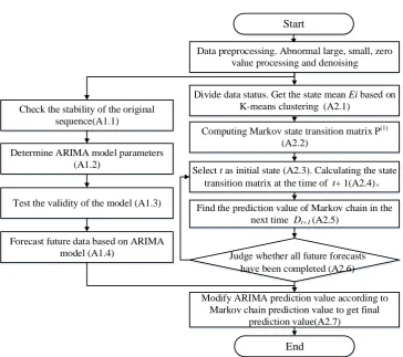
The daily water consumption prediction process based on the modified ARIMA prediction of Markov chain is demonstrated in figure 1, and the specific process is presented as algorithm 2, in Table 2.
Table 2. Algorithm of data forecast based on the Markov chain modified ARIMA model
Algorithm2: The proposed Markov chain modified ARIMA prediction
A2.1
The water consumption data series 𝐷𝑟 is divided into N states. The k-means clustering algorithm is used to cluster the data sequence, and the states of each value in the sequences, the partition of N states and the mean value Eiof state i are obtained.
A2.2
One step state transition matrix P(1) is calculated. According to the change of state in the sequence,
the state transition frequency 𝑓𝑖𝑗 is obtained, and then the transition probability 𝑝𝑖𝑗 of each state is obtained according to the formula (5).
A2.3 Select the time t as the initial state, and get the initial state vector 𝑋𝑡= (𝑥𝑡,1, 𝑥𝑡,2, ⋯ , 𝑥𝑡,𝑁). The data of the day before the forecast date is taken as the initial state.
A2.4
Calculate the state vector 𝑋𝑡+1 of water consumption to be predicted at the next time. Let 𝑥𝑡+1,𝑖 represent the probability of state i at time t+1, then the state vector at time t+1 is the product of state vector at time t and transfer matrix, 𝑋𝑡+1= 𝑋𝑡𝑃(1)
A2.5 The prediction value 𝐷𝑡+1 of future time based on Markov chain is calculated, which is expressed as formula (6).
A2.6 Repeat steps A2.3-2.6 to find the predicted water consumption of Markov chain at each time to be predicted.
A2.7 The prediction value of water consumption data at the time of t+n is obtained based on the Markov chain prediction value and the ARIMA prediction value by formula (7).
Figure 1. Flow chart of water consumption forecast based on Markov chain correction
4. Data analysis
The effectiveness of the proposed algorithm is verified by examples. The daily water intake data of some water monitoring points in Guangdong Province from 2016 to 2017 were selected for the experiment. The daily water consumption data from January to December 2016 was used to build the model, and the data from January 2017 was used to test the validity of the model.
4.1. Data pre-processing
The abnormal value in the daily water consumption data, such as the noise, zero value, abnormally large, or abnormally small value, may easily cause the error in the prediction model. Therefore, it is necessary to pre-process the data to remove the noise, abnormal large value, and other abnormalities. First, the abnormal large value of water consumption data was removed, based on the pauta criterion, and the mean value was used to fill the abnormal value. For the noise data, the mode decomposition method was used to remove the high frequency data component as the noise.
Figure 2 and figure 3 represent the original data and outliers processed data of the two monitoring points, respectively. Figure 4 and figure 5 demonstrate the outliers processed and de-noised data of two monitoring points, respectively.
Start
Divide data status. Get the state mean Ei based on K-means clustering (A2.1)
Computing Markov state transition matrix P(1) (A2.2)
Select t as initial state (A2.3). Calculating the state transition matrix at the time of t+ 1(A2.4)。
Find the prediction value of Markov chain in the next time Dt+1 (A2.5)
Judge whether all future forecasts have been completed (A2.6)
Modify ARIMA prediction value according to Markov chain prediction value to get final
prediction value(A2.7)
Data preprocessing. Abnormal large, small, zero value processing and denoising
End
Check the stability of the original sequence(A1.1)
Determine ARIMA model parameters (A1.2)
Test the validity of the model (A1.3)
Figure 2. The original data and data after removing outliers of monitoring point 1
Figure 3. The original data and data after removing outliers of monitoring point 2
Figure 5. Data after removing outliers and after de-noising of the monitoring point 2
4.2. Model validation
Firstly, the ARIMA analysis was performed on data 1 of the monitoring point. The water consumption data X1 of the monitoring point 1 fluctuates within a wide range. To eliminate the
fluctuation trend of its time series, data sequence of X1 is differentially processed and data sequence
of DX1 is obtained. As it can be seen from figure 6 the sequence after the first-order difference
fluctuates steadily, around the mean value. Figure 7 displays the autocorrelation diagram after the first-order difference of the water consumption sequence. It can be seen from the figure that the autocorrelation coefficient is greater than zero for a long time, indicating that the presence of a strong property between the sequences. The stationary state of the ADF unit root test sequence was selected (see Table 3.). The p-value of the unit root test is less than 0.05, suggesting the sequence after the first difference is a stationary sequence.
Figure 7. Autocorrelation chart of water consumption difference at the monitoring point 1
Table 3. The unit root test results of the water consumption data difference at monitoring point 1
ADF Critical value P value test 1% 5% 10%
-6.99 -3.45 -2.87 -2.57 7.72E-10
Table 4. The white noise test results of the water consumption data difference at monitoring point 1
Stat 5% 312.49 6.26E-70
The ARIMA model is fitted on the first-order stationary white noise sequence. The relative optimal model identification method is used to calculate the BIC information of all combinations of ARIMA (p, 1, q) at p, q less than or equal to 5. The model parameter with the minimum BIC information is selected and the BIC matrix bic_mat is as follows:
[
6808.99 6334.83 𝑁𝑎𝑁 𝑁𝑎𝑁 𝑁𝑎𝑁
6092.91 𝑁𝑎𝑁 𝑁𝑎𝑁 𝑁𝑎𝑁 𝑁𝑎𝑁
5376.16 5247.25 5214.20
5184.98 5180.17 5185.55
5178.98 5184.73 5190.27 5184.70 NaN NaN 𝑁𝑎𝑁 5189.91 5193.39 ]
(9)
When p value is 2 and q value is 2, the minimum BIC value is 5178.98. Then the sequence was fitted and analysed with model of ARIMA (2,1,2). The p value of white noise test around the residual is 0.93, which is a white noise, therefore the model is valid.
with model of ARIMA (2,1,2). The white noise test p value of the residual is 0.90, which is white noise, thus the model passes the test and is valid.
Figure 8. The original and first-order difference of total water consumption at monitoring point 2
Figure 9. Autocorrelation chart of water consumption difference at monitoring point 2
Table 5. The unit root test results of water consumption data difference at monitoring point 2
ADF Critical value P value test 1% 5% 10%
-8.18 -3.45 -2.87 -2.57 8.06E-13
Table 6. The white noise test results of water consumption data difference at monitoring point 2
Stat 5% 316.44 8.62E-71
Firstly, based on the Markov model, the training data is counted, and the state transition matrix and the one-step state transition value under each state are obtained. Subsequently, the future data prediction value is obtained as the future data trend. Then, the modified values are calculated, based on the prediction results of the Markov model.
In the prediction based on the Markov chain, the state of data sequence is set to 5, and K-means algorithm is used to divide the state of data sequence. The cluster diagram of water consumption of monitoring point 1 and 2 are demonstrated in Figure 10 and Figure 11 respectively. The cluster centre points of monitoring point 1 are the vector of: [127561.19 86415.6 120963.62 109515.03 139121.21].
Figure 10. Data clustering of monitoring point 1
Figure 11. Data clustering of monitoring point 2
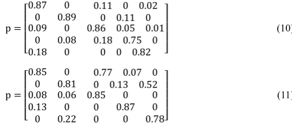
The Markov chain 1-step state probability matrix of daily water consumption data at monitoring point 1 and point 2 are presented in the following formula, respectively, as follows:
p =
[
0.87 0 0.11 0 0.02
0 0.89 0 0.11 0
0.09 0 0.18
0 0.08
0
0.86 0.05 0.01 0.18 0.75 0
0 0 0.82 ]
(10)
p =
[
0.85 0 0.77 0.07 0
0 0.81 0 0.13 0.52
0.08 0.13 0
0.06 0 0.22
0.85 0 0
0 0.87
0 0 0 0.78]
(11)
Given the significance level 𝛼 = 0.01, χ0.012 ((5 − 1)2) =32 can be obtained by looking up the table. According to equation (2) and
If the water consumption data of monitoring point 1 on that day is known, the state vector is set as P0 = [0, 0, 0, 0, 1], according to the water consumption data, then the state vector of the next day is P1=𝑃0 × 𝑃(1). According to equation
(6), the predicted value is [127114.01 88890.54 121126.54 109786.08 137019.38]. In the same way, the prediction value of the next n days is calculated, accordingly, based on the method of the modified ARIMA using Markov, that is, combining the predicted value of Markov chain to modify the predicted result of the ARIMA in proportion.
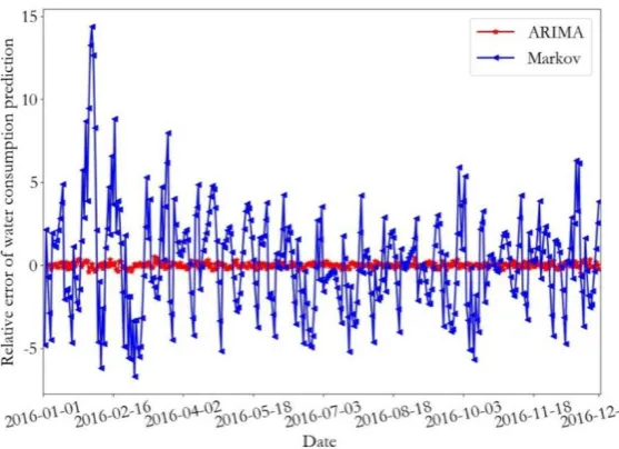
To test the prediction performance of the proposed model, the following prediction algorithms are compared and analysed, which includes the ARIMA prediction, the Markov prediction, and the data prediction method based on the modified ARIMA using Markov (ARIMA-M).
In order to measure the stability and adaptability of the prediction model, root mean square error (RMSE) and coefficient of determination (R2), and the relative prediction error (RE) are selected as the evaluation indexes. The RMSE reflects the difference between the original value and the estimated value. The smaller the value is, the closer the predicted value is to the real value, and the better the prediction effect is. The R2 can represent the whole fitting degree of the prediction model. The closer the R2 is to 1, the better the fitting degree of the prediction value to the observation value is, and the better the prediction performance of the model is. The RE is the ratio of absolute error to the real value. The relative error reflects the reliability of the prediction. If the true real value and the predicted value of data r are Ti and Yi, respectively, N is the number of predicted samples, and the
average value of all data values is 𝑇̅𝑖, then RMSE can be calculated through equation (12) , and R2 and RE can be expressed by equation (13) and (14) respectively.
𝑅𝑀𝑆𝐸 = √1
𝑁∑ (𝑇𝑖− 𝑌𝑖) 2 𝑁
𝑖=1 (12)
𝑅2= 1 −∑𝑁𝑖=1(𝑇𝑖−𝑌𝑖)2
∑𝑁𝑖=1(𝑇𝑖−𝑇̅ )𝑖2
(13)
𝑅𝐸 = ∑ (𝑇𝑖−𝑌𝑖)
𝑇𝑖
𝑁
𝑖=1 ×
1
𝑁× 100 (14)
Figure 12. Prediction results from the training data, at monitoring point 1
Figure 13. The relative error of the training data, at monitoring point 1
Figure 14. The relative error of the training data, at monitoring point 2
Table 7 and 8 show the prediction error of the ARIMA and the Markov model, on the training data set for monitoring point 1 and 2, respectively. According to the prediction data of monitoring point, the relative error (RE) of the ARIMA prediction is less than 0.2, and coefficient of determination R2 is close to 1, therefore, the training data set can be better fitted by this model. The training data mean square error, coefficient of determination, and relative error rate of the Markov model are much larger than those of the ARIMA model. The relative errors of the Markov model for monitoring point 1 and monitoring point 2 are about 13 and 18 times of the ARIMA, respectively. Therefore, the ARIMA model provides good fitting results for the training data, and the relative error RE of the Markov prediction is less than 2.5%, which can meet the requirements of the daily water consumption data prediction.
Table 7. Prediction error of the training set, at monitoring point 1
RMSE R2 RE ARIMA 275.17 0.9994 0.19 Markov 3919.08 0.90 2.47
Table 8. Prediction error of the training set, at monitoring point 2
RMSE R2 RE ARIMA 300.93 0.9996 0.13 Markov 5628.25 0.89 2.34
Therefore, the ARIMA and Markov combined data prediction model (ARIMA_M) can be used for the daily water consumption data prediction. The ARIMA model can fit the training data, with high prediction accuracy. The Markov model can predict the trend of water consumption data, based on the training data of water consumption.
Based on the training set of daily water consumption, the ARIMA and Markov prediction models can be obtained by training. The ARIMA and the proposed ARIMA-M correction algorithm are used to predict the data of 20 days from January 1 to January 20, 2017, to verify the validity of the model.
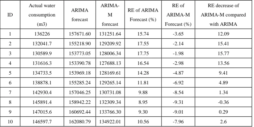
Table 9. Forecast value of monitoring point 1, during the next 10 days
ID
Actual water consumption
(m3)
ARIMA forecast
ARIMA-M forecast
RE of ARIMA Forecast (%)
RE of ARIMA-M Forecast (%)
RE decrease of ARIMA-M compared
with ARIMA 1 136226 157671.60 131251.64 15.74 -3.65 12.09 2 132041.7 155218.90 129209.92 17.55 -2.14 15.41 3 130589.9 153773.05 128006.34 17.75 -1.98 15.77 4 131616.3 153390.78 127688.13 16.54 -2.98 13.56 5 134733.5 153969.18 128169.61 14.28 -4.87 9.41 6 138878.1 155285.24 129265.14 11.81 -6.92 4.89 7 142930.4 157046.25 130731.08 9.88 -8.54 1.34 8 145891.4 158942.22 132309.34 8.95 -9.31 -0.36 9 147015.6 160692.44 133766.30 9.30 -9.01 0.29 10 146597.7 162080.79 134922.01 10.56 -7.96 2.6
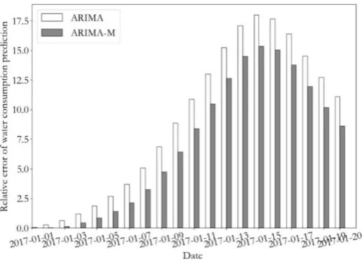
Figure 16 represents the total water consumption change and the relative error curve of monitoring point 2, during the next 20 days. Figure 17 shows the prediction error curve of water consumption of monitoring point 2, during the next 20 days using the ARIMA and ARIMA-M algorithm. It can be seen from the figure that the predicted value of the test data using the ARIMA-M model is closer to the real value, and the prediction error is lower.
Figure 17. The relative error of total water consumption prediction, at monitoring point 2 The prediction error of the ARIMA and the proposed ARIMA-M model in the overall test set of monitoring points 1 and 2 are presented in table 10 and 11, respectively. It can be observed from the table that compared to the training data, the prediction error of the test data is greatly increased. At monitoring point 1, the RMSE reaches to 14085, the R2 value is only -0.04, and relative error reaches to 8.07. Using the ARIMA-M, RMSE of the predicted value of test set is decreased by 25%, R2 is increased by more than 10 times, and relative error is decreased by 24.4%, in comparison with the traditional ARIMA. For monitoring point 2, compared to the ARIMA, RMSE of predicted value on ARIMA-M test set and the relative error are reduced by 18.4% and 13%, respectively.
Table 10. Prediction error of test set for monitoring point 1
RMSE R2 RE ARIMA 14085.60 -0.04 8.07 ARIMA-M 10569.32 0.42 6.10
Table 11. Prediction error of test set for monitoring point 2
RMSE R2 RE ARIMA 18388.74 -3.04 8.07 ARIMA-M 15003.34 -1.69 7.02
According to the above analysis, the ARIMA model can provide a better fit for the changes of daily water consumption data of monitoring points, while, the Markov can predict the trend of daily water consumption data within a certain error range. However, due to the randomness nature of the water consumption data, the prediction accuracy of the above model for the unknown data decreases, and the proposed ARIMA-M model can be used (1) to correct the deviation of the future daily water consumption prediction data, (2) to reduce the over fitting of the ARIMA model on the training data set, (3) to improve the prediction accuracy of the data, and (4) to provide data support for the decision makers, based on daily water consumption data prediction value.
5. Discussion
trend of the data, the ARIMA model was modified, which corrected the great error, caused by error superposition, and improved the accuracy of data prediction. This study analyses the actual daily water consumption data, on data monitoring point, and proposes a method based on the Markov correction prediction error, which can effectively improve the prediction accuracy of the future daily water consumption data of monitoring point.
For future research, the seasonal characteristics of water consumption data can be analysed, with the aim of further improvement in the prediction accuracy. In addition, the adaptability of the model to the annual water consumption data requires further exploration.
Author Contributions: Conceptualization, Hongyan Du, and Zhihua Zhao; methodology, Hongyan Du.; software, Hongyan Du; validation, Hongyan Du; formal analysis, Hongyan Du; investigation, Hongyan Du; resources, Hongyan Du; data curation, Hongyan Du; writing—original draft preparation, Hongyan Du; writing—review and editing, Hongyan Du; visualization, Hongyan Du; supervision, Hongyan Du; project administration, Hongyan Du; funding acquisition, Huifeng Xue. All authors have read and agreed to the published version of the manuscript.
Funding: This research was funded by the National Natural Science Foundation of China and Science, grant number U1501235 and the Science and Technology Program of Guangdong Province, grant number 2016B010127005.
Conflicts of Interest: The authors declare no conflict of interest. The funders had no role in the design of the study; in the collection, analyses, or interpretation of data; in the writing of the manuscript, or in the decision to publish the results.
References
1. Yasar A; Bilgili M; Simsek E. Water Demand Forecasting Based on Stepwise Multiple Nonlinear Regression Analysis. Arabian Journal for Science and Engineering 2012, 37, 2333-2341.
2. Mays LW. Water demand forecasting: McGraw-Hill, 1992.
3. Brekke L; Larsen MD; Ausburn M et al. Suburban Water Demand Modeling Using Stepwise Regression. J. - Am. Water Works Assoc. 2002, 94, 65-75.
4. Zhang Y; Liu Q; Feng C. Application of multiple linear regression analysis in predicting urban water demand in Beijing. Water supply and drainage. 2003, 29, 26-29.
5. Bennett C; Stewart RA; Beal CD. ANN-based residential water end-use demand forecasting model. Expert Syst. Appl. 2013, 40, 1014-1023.
6. Liu H; Zheng B; Jiang B. Prediction method of urban hourly water consumption based on artificial fish swarm neural network. Journal of Tianjin University (Science and Technology). 2015, 48, 373-378.
7. Mouatadid S; Adamowski J. Using extreme learning machines for short-term urban water demand forecasting. Urban Water J. 2016, 14, 630-638.
8. Donkor EA, Mazzuchi TA, Soyer R, et al. Urban Water Demand Forecasting: Review of Methods and Models. J. Water Resour. Plann. Manage. 2014, 140, 146-159.
9. Box G; Jenkins GM. Holden-Day Series in Time Series Analysis. Holden-Day San Francisco: CA, USA, 1976. 10. Shvartser L, Shamir U, Feldman M. Forecasting Hourly Water Demands by Pattern Recognition Approach.
J. Water Resour. Plann. Manage.1993, 119, 611-627.
11. Mombeni HA; Rezaei S; Nadarajah S, et al. Estimation of Water Demand in Iran Based on SARIMA Models. Environmental Modeling & Assessment. 2013, 18, 559-565.
12. Zhao L, Zhang J, Chen T. Application of product season ARIMA model to the forecast of urban water supply. Journal of Water Resources and Water Engineering. 2011, 22, 58-62.
13. Wu Z, Huang NE. A study of the characteristics of white noise using the empirical mode decomposition method. Proceedings of the Royal Society of London, Series A: Mathematical, Physical and Engineering Sciences. 2004, 460, 1597-1611.