A genetic algorithm Bayesian network approach for the analysis of metabolomics and spectroscopic data: application to the rapid detection of Bacillus spores and identification of Bacillus species

approach for the analysis of metabolomics 

and spectroscopic data: application to the 

rapid detection of Bacillus spores and 

identification of Bacillus species

Correa, E and Goodacre, R

http://dx.doi.org/10.1186/1471­2105­12­33

Title

A genetic algorithm­Bayesian network approach for the analysis of 

metabolomics and spectroscopic data: application to the rapid detection of 

Bacillus spores and identification of Bacillus species

Authors

Correa, E and Goodacre, R

Type

Article

URL

This version is available at: http://usir.salford.ac.uk/41380/

Published Date

2011

USIR is a digital collection of the research output of the University of Salford. Where copyright 

permits, full text material held in the repository is made freely available online and can be read, 

downloaded and copied for non­commercial private study or research purposes. Please check the 

manuscript for any further copyright restrictions.

For more information, including our policy and submission procedure, please

M E T H O D O L O G Y A R T I C L E

Open Access

A genetic algorithm-Bayesian network approach

for the analysis of metabolomics and

spectroscopic data: application to the rapid

identification of Bacillus spores and classification

of Bacillus species

Elon Correa

, Royston Goodacre

Abstract

Background:The rapid identification ofBacillusspores and bacterial identification are paramount because of their implications in food poisoning, pathogenesis and their use as potential biowarfare agents. Many automated analytical techniques such as Curie-point pyrolysis mass spectrometry (Py-MS) have been used to identify bacterial spores giving use to large amounts of analytical data. This high number of features makes interpretation of the data extremely difficult We analysed Py-MS data from 36 different strains of aerobic endospore-forming bacteria encompassing seven different species. These bacteria were grown axenically on nutrient agar and vegetative biomass and spores were analyzed by Curie-point Py-MS.

Results:We develop a novel genetic algorithm-Bayesian network algorithm that accurately identifies sand selects a small subset of key relevant mass spectra (biomarkers) to be further analysed. Once identified, this subset of relevant biomarkers was then used to identifyBacillusspores successfully and to identifyBacillus species via a Bayesian network model specifically built for this reduced set of features.

Conclusions:This final compact Bayesian network classification model is parsimonious, computationally fast to run and its graphical visualization allows easy interpretation of the probabilistic relationships among selected

biomarkers. In addition, we compare the features selected by the genetic algorithm-Bayesian network approach with the features selected by partial least squares-discriminant analysis (PLS-DA). The classification accuracy results show that the set of features selected by the GA-BN is far superior to PLS-DA.

Background

Bacillus and Clostridiumspecies can adapt to rapidly

changing environments and starvation by developing spores. An endospore is a dormant non-reproductive structure produced by these Gram-positive bacteria and is a survival mechanism adapted to spending a long per-iod of time in hostile conditions. The sporulation

pro-cess in Bacillusspecies causes singular molecular and

cellular changes in the cell which are not seen in the vegetative state [1]. One of these changes is the

biosynthesis of calcium dipicolinate, which is found in sporulated cells but not in the vegetative ones.

Members of the genusBacillus are widely distributed

in the environment and because their spores are so resistant their control is of considerable importance in the food manufacture [2]. Some of these bacteria are

pathogenic including B. cereusand B. subtilis which

cause food poisoning. The most notorious member of

this genus is B. anthracis, which is the causal agent of

anthrax, and the rapid identification of spores and bac-terial identification are paramount because of its impor-tance as a potential biological warfare agent [3] and in bioterrorism [4]. Thus there is a need to have a generic

* Correspondence: [email protected] 1

School of Chemistry, The University of Manchester, 131 Princess Street, Manchester, M1 7ND, UK

Full list of author information is available at the end of the article

characterisation method that allows rapid identification of spores and typing of bacteria.

Many automated analytical techniques such as Raman spectroscopy [5], liquid and gas chromatography [6,7] and Curie-point pyrolysis mass spectrometry (Py-MS) [8-10] have been used to identify bacterial spores. All of these methods rely on chemometric analyses of the data and the question arises as to how robust these mathe-matical models are. However, the vast majority of

mod-elling approaches are considered“black boxes” as they

do not readily allow the specific association between input analytical data and output classification to be revealed.

These types of data analysis involve a large number of features to be analysed, such as several mass spectra. This high number of features makes interpretation of the data extremely difficult Therefore, we start our data analysis by reducing data dimensionality. This data reduction step selects a small subset of key relevant masses to be further analysed and discards the less important ones. This feature selection procedure uses Bayesian network learning methods coupled with genetic algorithms to identify bacterial spores and clas-sifyBacillusspecies.

A Bayesian network (BN) is basically a graphical model of a probability distribution over a set of variables of a given problem domain [11,12]. This graphical model provides a compact and intuitive representation of the relationships among variables of a given problem domain. Nodes on the graph represent variables from

the problem (e.g.,m/zintensities) and an arrow linking

two nodes indicates a statistical correlation between them. This statistical correlation falls broadly into one

of the two categories: (a) “positive correlation”indicates

that the values of both variables increase or decrease

together, and (b)“negative correlation” indicates that as

one variable increases, the other decreases, orvice versa.

The network structure of a BN encodes probabilistic dependencies among domain variables and a joint prob-ability distribution quantities the strength of these dependencies [13]. The resulting graphical model or network has two main uses. (1) Visualization of prob-abilistic relationships: the graphical model provides direct and accurate information about the underlying

interactions among variables of interest, m/zintensities

in our case, and (2) Inference: the Bayesian network is intrinsically an inference model and can be used to pre-dict outputs or to classify new samples.

We use statistical and data mining algorithms to iden-tify Bacillusspores automatically from their Curie-point pyrolysis mass spectrometry data. This process extends the data mining analysis to a two step hierarchical-based classification that further identifies the bacilli into one of their respective species. First, the data dimensionality

is reduced by a feature selection process using genetic algorithms (GA) and BNs in parallel. Subsequently, once that the relevant variables are identified, a classification model using only BN is built based on the reduced data set, and this process undergoes full validation. Next a statistical analysis of the interactions among variables and classes and variables and variables is performed using the built Bayesian network model. As this

com-bined process identifies probabilisticbiomarkers in the

data set it is possible to develop predictive, testable models that allow inference of biological properties of the bacilli. The computer code for the GA-BN algorithm developed on this work was written in R programming language [14] ver. 2.9.2 and is freely available, together

with theBacillusdata set, on request to the

correspond-ing author.

Methods

TheBacillusdata set

The work uses theBacillusPy-MS data set reported in

[8] and described as an additional file (see Additional file 1). Unlike most data sets which concentrate on a

single or only a handful of Bacillusspecies, this data set

investigates 36 different strains of aerobic endospore-forming bacteria encompassing seven different species:

Bacillus amyloliquefaciens, Bacillus cereus, Bacillus licheniformis, Bacillus megaterium, Bacillus subtilis (including Bacillus niger and Bacillus globigii), Bacillus sphaericus, and Brevibacillus laterosporus. These bac-teria were grown axenically on nutrient agar as detailed in [8,15] and vegetative biomass and spores were ana-lyzed in triplicates by Curie-point Py-MS. The data set

contains 216 Bacillus samples; 108 are vegetative and

108 are sporulated. For a more detailed explanation of this data set see [8]. A phylogenetic tree of the type

strains of theBacillusspecies studied in this paper can

be found in [16].

Data analysis

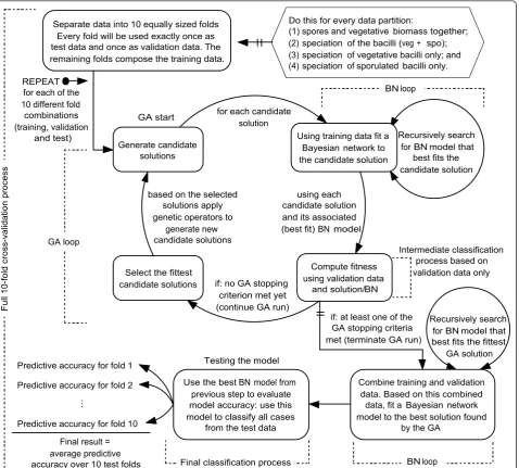
The overall work flow for the data analysis is shown in Figure 1 and involved a two stage process. The input data sets for the data analysis contained the full Py-MS

spectra, 150 m/zintensities. The data were normalised

as a percentage of the total ion count to remove the

influence of sample sizeper se.

Stage 1 employed a genetic algorithm for feature

selection with classification of (a) either spores versus

searches for an optimal feature subset tailored to a particular algorithm, such as a Bayesian network. For more information on wrapper and other feature selec-tion approaches see [17].

Stage 2involved the fitting of a new Bayesian network model to the best GA solution found on the previous stage. The built BN model is then used to determine

probabilistic relationships between the m/z intensities

selected by the GA and the classification (sporulation status or speciation). This two step process and model validation are detailed below.

Genetic algorithms (GAs)

A GA is an optimization procedure that evolves a popu-lation of candidate solutions to solve an objective func-tion [18]. A GA repeatedly applies operators based on natural selection and genetic recombination to the can-didate solutions. In a standard GA the initial solutions are randomly generated using a uniform distribution. The candidate solutions are called chromosomes. The chromosomes are usually represented by fixed-length strings over a finite alphabet. The term fitness is used to describe the quality of a candidate solution. The fitness

Testing the model

...

Predictive accuracy for fold 10

Intermediate classification process based on validation data only

Recursively search for BN model that best fits the fittest

GA solution

Final result = average predictive accuracy over 10 test folds

if: at least one of the GA stopping criteria met (terminate GA run) GA start

based on the selected solutions apply genetic operators to

generate new candidate solutions

if: no GA stopping criterion met yet (continue GA run)

using each candidate solution and its associated (best fit) BN model

Recursively search for BN model that

best fits the candidate solution for each candidate

solution

Compute fitness using validation data

and solution/BN Select the fittest

candidate solutions

Using training data fit a Bayesian network to the candidate solution

Combine training and validation data. Based on this combined data, fit a Bayesian network model to the best solution found

by the GA Use the best BN model from

previous step to evaluate model accuracy: use this model to classify all cases

from the test data

BN loop

Final classification process BN loop

GA loop

Full

10-fold cross-validation process

Separate data into 10 equally sized folds Every fold will be used exactly once as test data and once as validation data. The remaining folds compose the training data.

Predictive accuracy for fold 1

Generate candidate solutions

Predictive accuracy for fold 2

Do this for every data partition:

(1) spores and vegetative biomass together; (2) speciation of the bacilli (veg + spo); (3) speciation of vegetative bacilli only; and (4) speciation of sporulated bacilli only.

for each of the 10 different fold combinations (training, validation

and test) REPEAT

is a measurement of how well the chromosome solves the objective function. The fitness associated with a chromosome is used to select probabilistically which chromosomes from the population will recombine and possibly generate new solutions. A genetic operator called crossover is applied to create two new chromo-somes (progeny) from a pair of selected chromochromo-somes called parents. The crossover consists of swapping ran-dom subsets of the genetic material from both parents. Because of the selective pressure applied on the popula-tion through a number of generapopula-tions, the overall trend is towards higher-fitness chromosomes. Mutations are used to help preserve diversity in the population by introducing random changes into the chromosomes. Both crossover and mutation are usually applied with user-defined probabilities, and in general, the probability of crossover is much larger than the probability of mutation. For more details on genetic algorithms see [19-21]. The design of our genetic algorithm is as fol-lows. We employed a binary chromosome with 150 bits,

one for eachm/z variable. A gene value of 1 indicates

that the corresponding m/z variable is selected and a value of 0 indicates that it is not selected. A population size of 200 candidate solutions was used, with a cross-over and mutation probabilities of 0.75 and 0.033, respectively. During the test phase of the GA these para-meters generated the best results; but we make no claim that they are optimal parameter values. Setting the para-meters of a GA is not a trivial task and GA parameter optimization is a topic for future investigation. The objective function that we employed was to maximize classification accuracy. The fitness of a candidate solu-tion was assessed as the classificasolu-tion accuracy, on a validation set, achieved by the BN model built for the candidate solution being assessed. As each candidate

solution represents a different subset of features (m/z

intensities), the BN model built for a particular solution is a classification model based solely on the features pre-sent on that solution, e.i., the features that correspond to the genes whose value is equal to 1 inside the chro-mosome, Figure 1. The stopping criteria used were: (1) maximum of 200 generations are performed on a single GA run, (2) a solution whose classification model (BN) produces 100% of predictive accuracy is found, or (3) when all the 200 solutions in the population converge to a single solution.

Bayesian networks (BNs)

A BN is a graphical map of the probabilistic relation-ships among variables of a given problem domain [22]. The graphical representation of a BN is a directed

acyc-lic graph. A directed acycacyc-lic graphGis an ordered pair

G=(V; E) where V is a set whose elements are called

vertices or nodes and E is a set whose elements are

called directed edges, arcs, or arrows. The graphG

con-tains no directed cycles; for any vertexυÎV, there is no

directed path that starts and ends on υ. An example of

a Bayesian network is as follows. This is a modified

ver-sion of the so-called “Asia”problem found in [23].

Sup-pose that a doctor is treating a patient who has been suffering from shortness of breath, called dyspnoea. The doctor knows that diseases such as tuberculosis, bron-chitis and lung cancer are possible causes of this. The doctor also knows that other relevant information includes whether the patient is a smoker, which increases the chances of lung cancer and bronchitis, and what sort of air pollution the patient has been exposed to. A positive X-ray would indicate either tuberculosis or lung cancer. The set of variables for this problem and their possible values are shown in an additional file (see Additional file 2) together with a Bayesian network representing this problem. The network structure, also known as network topology, shows how variables

corre-late to each other. More formally, let X= {X1,X2,..., Xn}

be a multivariate random variable whose componentsXi

are also random variables. A corresponding lower-case

letter xidenotes an assignment of state or value to the

random variable. Xi Parents (Xi) represents the set of

nodes that have a directed edge pointing toXi.

Consider a BN containing n nodes, X1 toXn, taken

in that order. A particular value of X = {X1,X2,..., Xn}

in the joint probability distribution is represented by

p(X) =p(X1 =x1, X2 =x2, ..., Xn =xn), or more

com-pactly,p(x1, x2, ...,xn). The chain rule of probability

the-ory allows the factorization of joint probabilities, therefore:

p p x p x x p x x x

p x x x

n n

i i

i

( ) ( ) ( | )... ( | ,..., ) ( | ,..., )

X 









As the structure of a BN implies that the value of a particular node is conditional only on the values of its parent nodes, Equation 1 is reduced to:

p p Xi Parents Xi

i

( )X 



Learning the structure of a BN is an NP-hard problem [24,25]. Many algorithms developed to this end use a scoring metric and a search procedure. The scoring

metric evaluates the“goodness-of-fit” of a structure to

algorithm adds to the current network the edge that most increases the score of the new resulting network. The search stops when no other edge addition improves the score of the network. Additional file 3 shows the pseudocode of a generic greedy search algorithm for learning Bayesian network structures. In this paper, we use an unconventional scoring metric to evaluate the

goodness-of-fit” (score) of a network structure to the

data. The scoring metric adopted is specific to our clas-sification task and is computed as follows. The entire data set is divided into mutually exclusive training and

test sets, see “Model validation” for more details. The

training set is further divided into two mutually exclu-sive parts - training and validation sets. The first part (training set) is used to compute the probabilities for the Bayesian network. The second part is used as the validation set. During the search for the best possible network structure only the validation set is used to compute predictive accuracy and the measurement (quality) of the predictive accuracy achieved is used as the scoring metric for the Bayesian network model pro-posed. The higher the predictive accuracy value, the bet-ter the BN model fits the data. Once the best GA solution is found, at the end of the GA run, the valida-tion set and the training set are merged and this merged data (i.e., the entire original training set) is used to com-pute the probabilities for a new BN fitting to this data. Using this newly built BN model the predicted accuracy, for that combination of folds, is then computed on the previously untouched test set. The results reported in this paper are the average predictive accuracy over 10 entirely distinct test folds.

To summarize, the Bayesian network is used both in parallel to the GA and sequentially after each complete

GA run is performed as shown in Figure 1. First, the

parallel GA-BN usage. For each new GA solution the

following procedure is repeated. Solution Sk is

gener-ated. A Bayesian network modelBkis built based only

on the features (m/z variables) that are selected inSk

and using the training set to compute probabilities. The

model Bk is then used to predict the samples on the

validation set and the predictive accuracy produced by

Bk becomes the fitness value of solutionSk, i.e., fitness

value of Sk = predictive accuracy resulting from model

Bk. At the end of the GA run, the solution with the

highest fitness value Sbest is retained. Second, the

sequential BN usage after the complete GA-BN run.

A new Bayesian networkBbestis built based onSbestbut

this time using the combined data, training set + valida-tion set, for computavalida-tion of probabilities. The predictive

accuracy ofBbestis then evaluated on a third, previously

untouched fold, the test set. This result is then added to the computation of the average accuracy over the

10-fold cross-validation. The process is repeated for each of the 10 folds.

Feature selection

Many data mining applications involve the task of build-ing a model. The goal of such a model is to classify data records according to a set of common features. Feature selection, also known as variable or attribute selection, is the technique of selecting a subset of relevant vari-ables for building robust and accurate learning models. In the present work, feature selection using GA is used to reduce data dimensionality before a classification model is built. The reduction of the number of variables speeds up model building and improves model stability and interpretability. In addition, we independently applied a partial least squares-discriminant analysis [26,27] (DA) algorithm for feature selection. PLS-DA is a particular case of partial least squares regression where the dependent variable, or response, is a binary or a dummy variable. We use the PLS-DA implementation

form the R package “Classification and Regression

Training” (Caret) ver. 4.31 written by Max Kuhn [28].

The importance of every variable for the prediction model is measured by their variable importance for pro-jection (VIP) coefficient. Variables with large VIP, larger than 1, are the most relevant ones for the model and contribute more for class discrimination.

Model validation

examples in the validation set. When the run of the GA algorithm is completed, the training set (8 folds) and the validation set (1 fold) are merged into a full, bigger training set. This full merged training set is used to re-compute the probabilities for a new BN fitted to the best solution (subset of features) returned by the GA. The new Bayesian network is then used to classify examples in the test set (the 10th fold), which was never accessed before during the run of the genetic algorithm. The reasons for having separate validation and test sets are that in a classification model the goal is to measure predictive accuracy (generalization ability) on a test set unseen during training. Hence, the test set cannot be used by the GA, and is reserved just to compute the predictive accuracy associated with the Bayesian net-work built with the best set of variables selected at the end of the GA run.

Results and Discussion

Discriminating between different physiological states

First, a GA was used for the variable selection phase as detailed above. Thirty independent runs of the genetic algorithm were performed. Each individual run included a 10-fold cross-validation, therefore 300 randomly gen-erated folds were analyzed overall. All variables that appeared in 70% or more of the final GA solutions were selected, and this included 17, out of the 150 variables:

m/z 58,m/z 59, m/z 60,m/z 63, m/z 64,m/z 65, m/z

70,m/z76,m/z77, m/z79,m/z84,m/z90,m/z92,m/

z99,m/z105, m/z132 andm/z154. We chose a cutoff

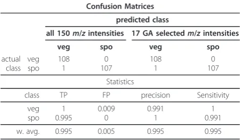
percentage of 70% for two main reasons: (1) to simplify the interpretation of the Bayesian network model by limiting the number of variables used to build the model, and (2) to concentrate the analysis only on the most relevant features from the data. After this variable selection two classification models were built using Bayesian networks. The first BN model is built using all 150 variables available; the second BN model is built

using only the 17 GA-selected variables. Table 1 shows the confusion matrices for both classification models and the statistics related to those matrices. TP and FP are the numbers of true positives and false positives respectively.

The results in Table 1 show an identical predictive accuracy for the classifications with either all 150 vari-ables or the reduced data (17 GA selected varivari-ables). In practice the classification model using only 17 variables should be favoured because it is less computationally expensive to run, more parsimonious [30], and also sim-pler to interpret. Whilst the variable selection and classi-fication model shows the most relevant variables for the

identification of Bacillus spores, it does not give any

information about how these variables correlate to the classes or indeed to each other. Therefore, we use

prin-cipal component analysis (PCA) to detect groups ofm/z

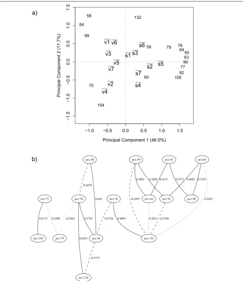
intensities that strongly correlate to each other and observe their relationships to the physiological state of the bacilli. Figure 2(a) shows the biplot for the average PC scores value of the 14 classes and overlaid on this

plot are them/z intensities from the PC loadings matrix.

The PC scores plot in Figure 2(a) shows a clear

separation between the vegetative ( )v and sporulated

(s) bacilli in the first PC which accounts for 46% of the

total explained variance. Them/zintensities that appear

to the right of the vertical dotted line that divides the graph have a strong correlation with the sporulated phy-siological state and the intensities to the left of that line are strongly correlated to the vegetative state. The

proximity of v1 and v6 on the graph indicates that in

their vegetative stateB. amyloliquefaciensandB. subtilis

are very closely related and this reflects the known tax-onomy of these two species [16]; these are also closely

related to the taxonomically similar B. licheniformis

(v3). This is also seen in the spores of these bacteria.

This suggests that despite choosingm/zthat can

discri-minate between spores and vegetative cells some infor-mation on the different species is still present. This is

also true for B. cereus (v2) and B. megaterium (v4)

that also co-cluster and are taxonomically similar [16].

To examine the interactions among the m/zintensities

further we have developed a powerful probabilistic model based on Bayesian networks. Contrary to intui-tion, the direction of the arrows in a Bayesian network does not necessarily imply a cause-effect relationship between the variables; that is to say a Bayesian network

is not a “causal network”. Thus to eliminate possible

confusion we have intentionally omitted the arrow heads from our BN graphs. Figure 2(b) shows the BN

describing the association of the 17 selectedm/z

intensi-ties, and as detailed above this was fully validated using

Table 1 Vegetative and sporulated classes: confusion matrices and summary statistics, w. avg. = weighted average

Confusion Matrices

predicted class

all 150m/zintensities 17 GA selectedm/zintensities

veg spo veg spo

actual class

veg spo

108 1

0 107

108 1

0 107

Statistics

class TP FP precision Sensitivity

veg spo

1 0.995

0.009 0

0.991 1

1 0.991

−1.0 −0.5 0.0 0.5 1.0 1.5

−

1.5

−

1.0

−

0.5

0.0

0.5

1.0

1.

5

Principal Component 1 (46.0%)

Pr

incipal Component 2 (11.7%)

v1

v2

v3

v4

v5

v6

v7

s1

s2

s3

s4

s5

s6

s7

59

60

63 64

65

70

76

77 79 84

90

92 99

105 132

154

m/z 77

m/z 105 0.8173

m/z 79 0.2498

m/z 65

m/z 92

0.6683

m/z 132

0.2432 m/z 90

0.3102

-0.2704 m/z 58

m/z 84 0.663 m/z 70

-0.3678

m/z 154 -0.2737 0.3767

0.6451 -0.2483

m/z 76

-0.2726 0.4983

m/z 63

0.4713

m/z 64 0.4151

0.2631 m/z 59

0.2849

-0.2697 0.3862

a)

b)

10-fold cross-validation. Solid lines indicate a positive correlation between nodes, dashed lines indicate nega-tive correlation and the thickness of the line indicates the strength of the correlation. Therefore the thicker the line is the stronger the correlation. The number beside the line shows the partial correlation coefficient for that correlation. A partial correlation estimates the correla-tion between two nodes when the effect of all other nodes in the model is held constant, and this process

avoids finding variables (m/z) that are not directly

cor-related to each other [31].

The network Figure 2(b) shows the correlation among

the m/z intensities. The strongest correlation on the

network is a positive correlation betweenm/z 105 and

m/z 77. m/z 105 is a pyridine ketonium ion known to

arise from DPA [8] and Beverlyet al., Havey et al. and

Opitz have suggested thatm/z77 results from the

elec-tron ionization fragmentation pathway via loss of CO

fromm/z 105 [32-34]. As thesem/z are highly

corre-lated in the BN and appear closer to the sporucorre-lated classes on Figure 2(a), the results indicate that for

sporulated bacilli them/z 105 andm/z 77 intensities are

noticeably higher than for the vegetative case.

In order to generate a rule for differentiating spores from vegetative cells we also applied a classification and regression trees algorithm (CART) implemented accord-ing to the methods described in [35] and written in R programming language [14]. The classification tree pro-cedure creates a tree-based classification model which classifies cases into groups. The procedure provides vali-dation tools for exploratory and confirmatory classifica-tion analysis. The CART algorithm produced a

classification tree containing only four biomarkers,m/z

63,m/z77,m/z84 andm/z105, as sufficient to

discrimi-nate accurately between the physiological states of the bacilli. We then proceeded to use discriminant analysis to produce a classification equation using those four m/z intensities. To compute such equation we used the

discri-minant analysis option in the software“Statistical

Pack-age for the Social Sciences”SPSS Inc. [36] ver. 16. The

equation coefficients are canonical discriminant coeffi-cients. The resulting formula is shown in Equation 3.

f MZ( )_ h 



vegetative, if 0,

spore, otherwise. (3)

where h= 3.523 m/z 63+ 4.193m/z 77 - 1.007 m/z

84 -0.347m/z105 -0.961, and MZ= (m/z63, m/z 77,

m/z 84 ;m/z 105). This equation successfully classifies

100% of the cases from the Bacillusdata set correctly.

Thus we have understood some of the relationships between the variables, confirmed that DPA and its pro-duct ions in Electron Impact Mass Spectrometry (EI-MS) are excellent biomarkers for spores and have a

very parsimonious model where only 4 of the original 150 ions are used to describe the solution adequately.

Discriminating between species

For this analysis the species are considered as classes

(n= 7). In order to ascertain whether there was any

dif-ference in classifications based on physiology, we per-formed these experiments using three different partitions of the mass spectral data. The first partition uses all the 216 bacilli collectively, vegetative + sporu-lated. The second partition uses only vegetative cells and the third one uses only sporulated cells. Experi-ments on the second and third partitions expect that one has already differentiated between the two physiol-ogy states (as illustrated above) and would work like a hierarchical classification were the physiological state of the cases is known and only the species have to be predicted.

The variable selection GA-classifier was applied to each of the three partitions of the data and produced the subsets of variables shown in the Venn diagram Figure 3.

The diagram, Figure 3, shows that for the data set

containing the 216 bacilli, labelled BOTH, 22m/z

inten-sities have been selected as relevant to discriminate

between the differentBacillus species, whereas for the

data set containing only vegetative cells and the data set containing only sporulated cells, 25 and 39 variables were selected respectively It is also clear that some ions

(m/z57, 67, 74, 89, 104 and 136) were used by all

classi-fiers irrespective of data partitioning.

Species as classes: all bacilli

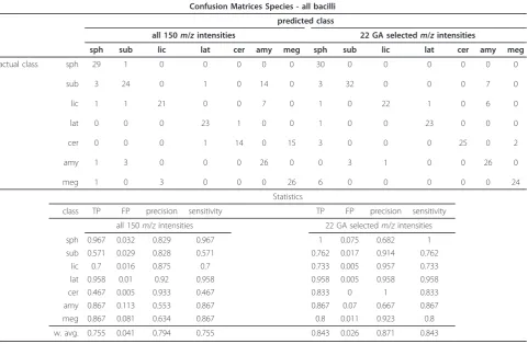
These experiments were aimed at classifying all the 216 Py-MS spectra from the bacilli into one of the seven possible species. Table 2 shows the confusion matrix for

this classification when all 150m/zions were employed

as well as the statistics related to these classifications. This table also details the results after GA variable selection down to the 22 ions highlighted in Figure 3. It is clear from the summary statistics (Table 2) that pre-diction was improved when only these 22 GA selected ions were used again highlighting the power of the fea-ture selection performed by the GA-Bayesian network algorithm (GA-BN).

Figure 4(a) shows the PC scores biplot for the average value of the classes and the associated PC loadings plot

which shows the influence of the m/z intensities

selected. This figure shows the classes and their

rela-tionship with them/z intensities. The intensitiesm/z 89,

m/z 136 andm/z65, for instance, are good

discrimina-tors for the speciesB. sphaericus ( )5s when theBacillus

is sporulated but not as good when this species is in

to ( )1s and of (3v) to ( )3s on the graph suggests that bacilli belonging to those respective species remain rela-tively similar regardless of their physiological state.

The Bayesian network model built on the 22 GA selected variables is shown in Figure 4(b). Interpretation of these relationships is difficult given the molecular nature of the ions in Py-MS (molecular ions are very rarely seen, rather complex pyrolysate and fragments thereof are detected but remain unidentified).

Despite this limitation of the data, rather than the BN, we see two separate sub-networks for species clas-sifying when both spores and vegetative cells are included in the BN analysis. These relationships are

not directly related to the differences between spores and vegetative cells, nor are these probabilistic rela-tionships among variables wholly mirrored in PC scores (Figure 4(a)), and we see a mixture of selected ions from the different areas of PCA. For example,

whilst m/z 89, 136, 65 are highly positively correlated

in both the BN and PCA the BN extends this network

via a negative correlation to m/z 108 and m/z 57

which are located diagonally opposite in the PC

load-ings plot, but not m/z 70 which is not used in the BN

at all. In addition, despite m/z 52 and 53 close

rela-tionship in PCA these are found to be separated in the BN. Thus this suggests that additional information

SPO VEG

BOTH

m/z 55, m/z 62

m/z 63, m/z 64

m/z 71, m/z 72

m/z 77, m/z 82

m/z 86, m/z 90

m/z 93, m/z 102

m/z 105, m/z 117

m/z 119, m/z 120

m/z 121

m/z 122

m/z 126

m/z 132

m/z 140

m/z 51

m/z 58

m/z 60

m/z 61

m/z 75

m/z 94

m/z 100

m/z 131

m/z 154

m/z 112

m/z 129

m/z 52

m/z 59

m/z 65

m/z 68

m/z 69, m/z 108

m/z 147, m/z 156

m/z 53

m/z 70

m/z 97

m/z 101

m/z 113

m/z 157

m/z 57

m/z 67

m/z 74

m/z 89

m/z 104

m/z 136

m/z 73

m/z 83

m/z 91, m/z 92

could be generated from the BN when compared to PC loadings plots, and this will be an area of future work using ions of known origin.

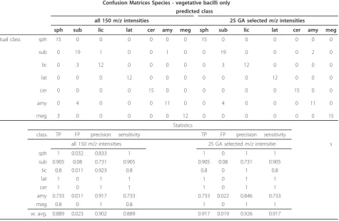
Species as classes: vegetative cells only

These experiments classified 108 mass spectra from the vegetative bacilli into one of the 7 possible species stu-died. Table 3 shows the confusion matrix for this classi-fication as well as the statistics related to this classification for both the full Py-MS spectrum and for the 25 ions selected using GA, and in this case the data reduction has not led to a significant improvement in classification.

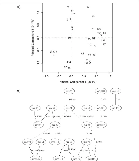
Figure 5(a) shows the PC scores biplot for the average

value of the classes and the associated m/z intensities

located in the PC loadings. This biplot was generated based on the 25 GA selected variables for this configura-tion of the data set and shows the locaconfigura-tions of the

spe-cies classes and their relationship with the m/z

intensities. These relationships mirror very well the expected taxonomy of these bacilli as 4 groups are seen: (1)B. subtilis, B. amyloliquefaciensandB. licheniformis, (2)B.cereusand B. megaterim, (3) B. sphaericusand (4)

B.laterosporus, and highlights that reduction of the data

has not comprised the known relationships between these bacteria.

The Bayesian network model built on the 25 GA selected variables is shown in Figure 5(b).

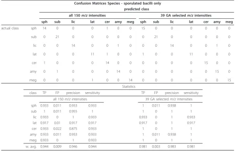
Species as classes: spores only

These experiments classified the Py-MS data from 108 sporulated bacilli into one of the 7 possible species stu-died. Table 4 shows the confusion matrix for these classifi-cations as well as the statistics related to this classification for both the full Py-MS spectra and the 39 GA selected ions. In contrast to the model made from the vegetative cells, the reduced ions for the spores shows an improve-ment in the predictive ability for this model, which is encouraging considering that previous studies have

sug-gested that the phenotype ofBacillusspecies on

sporula-tion, as measured using Py-MS, becomes more similar and hence one would expect the predictions for spores to be worse than for vegetative cells [37].

Figure 6(a) shows the PC score biplot based on the 39 GA selected variables for the average value of the classes

and the correspondingm/zintensities from the PC

load-ings matrix are also shown. In contrast to the same ana-lysis from the vegetative cells, the taxonomic

Table 2 Species: classification results for all bacilli (including vegetative and sporulated cases)

Confusion Matrices Species - all bacilli

predicted class

all 150m/zintensities 22 GA selectedm/zintensities

sph sub lic lat cer amy meg sph sub lic lat cer amy meg

actual class sph

sub lic lat cer amy meg 29 3 1 0 0 1 1 1 24 1 0 0 3 0 0 0 21 0 0 0 3 0 1 0 23 1 0 0 0 0 0 1 14 0 0 0 14 7 0 0 26 0 0 0 0 0 15 0 26 30 3 1 1 3 0 6 0 32 0 0 0 3 0 0 0 22 0 0 1 0 0 0 1 23 0 0 0 0 0 0 0 25 0 0 0 7 6 0 0 26 0 0 0 0 0 2 0 24 Statistics

class TP FP precision sensitivity TP FP precision sensitivity

all 150m/zintensities 22 GA selectedm/zintensities

sph 0.967 0.032 0.829 0.967 1 0.075 0.682 1

sub 0.571 0.029 0.828 0.571 0.762 0.017 0.914 0.762

lic 0.7 0.016 0.875 0.7 0.733 0.005 0.957 0.733

lat 0.958 0.01 0.92 0.958 0.958 0.005 0.958 0.958

cer 0.467 0.005 0.933 0.467 0.833 0 1 0.833

amy 0.867 0.113 0.553 0.867 0.867 0.07 0.667 0.867

meg 0.867 0.081 0.634 0.867 0.8 0.011 0.923 0.8

w. avg. 0.755 0.041 0.794 0.755 0.843 0.026 0.871 0.843

−1.0 −0.5 0.0 0.5 1.0 1.5

−

1.5

−

1.0

−

0.5

0.0

0.5

1.0

Principal Component 1 (24.3%)

Pr

incipal Component 2 (23.3%)

1v

2v

3v

4v

5v

6v

7v

1s

2s

3s

4s

_5s

6s

7s

52 53

57

59

65 67

68 69

70 74

89

97

101 104

108

112

113 ₁₂₉

136

147

156 157

m/z 156

m/z 157 0.711

m/z 53

m/z 97

0.6195

m/z 67 0.424

m/z 129 0.3157

m/z 68

m/z 69 0.4943

m/z 65

m/z 136

0.4751 m/z 89 0.2865

m/z 57

-0.2852

m/z 74 0.4425

m/z 112 -0.2931

m/z 113 0.4408 0.3159

m/z 101

0.3825

m/z 147 0.3486

0.3408

m/z 108

0.3713 0.3377 -0.3483

m/z 52

-0.2978

-0.338

a)

b)

Figure 4Species all bacilli. (a) principal component analysis discriminating among species (all bacilli). v = vegetative, s = sporulated, ₁

relationship between these bacilli whilst evident is more

diffuse; that is to say there is overlap betweenB.

lateros-porus ( )7 and theB. subtilislike cluster ( , , )1 3 6 . Fig-ure 6(a) raises some other interesting observations. First,

there is a suggestion that the cluster formed bym/z77,

m/z 105 andm/z122 could be related to the

fragmenta-tion pathway of benzoic acid as reported by [34,38].

Sec-ond,m/z77 and 105 are DPA related mass spectra [32]

and their proximity toB. cereuson the PCA plot could

indicate that B. cereushas a higher level of DPA than

the other 6 Bacillusspecies studied in this work. This

idea, however, seems to be contradictory. While some

studies such as [39] suggest that B. cereushas in fact a

high DPA level, higher than for B. megaterium, for

instance, other studies such as [40,41] indicate the con-trary. Although our PCA plot does seem to suggest that

B. cereus has a high DPA level (agreeing with [39]), clo-ser inspection of the data set tells a slightly different

story. It reveals that the average values form/z 77 and

m/z105 are higher forB. megateriumandB.sphaericus

than they are for B. cereus (agreeing with [40,41]).

Therefore, the reason why m/z77 and 105 are closer to

B. cereus on the PCA plot may be due to the fact that

B. cereus falls in-between B. megaterium and B.

sphaericus on the plot. The Bayesian network model

built on these 39 ions is shown in Figure 6(b) where the

strong correlation involving m/z 77,m/z 105 and m/z

122 is also highlighted.

GA-Bayesian network vs. PLS-DA

To assess the power of the proposed GA-BN method as a feature selection technique we compare it to PLS-DA. Using exactly the same partitions of the data set assessed by the GA-BN algorithm, we applied PLS-DA to identify the most relevant features in each of those partitions. We then computed the new classification results based on those features selected by PLS-DA. Table 5 reports the following classification results: (1) the weighted true positive rate, (2) the total number of variables selected, and (3) the percentage of variables selected by PLS-DA that have also been selected by

GA-BN, described as “overlap”. The true positive rates from

Table 5 show that variables selected by GA-BN separate the classes more accurately than the variables selected by PLS-DA, in all cases. In particular, the results suggest that as the number of classes increases, from 2 for phy-siological state to 7 to the other cases, the classification accuracy obtained by PLS-DA decreases noticeably. For

Table 3 Species: classification results for vegetative bacilli only

Confusion Matrices Species - vegetative bacilli only predicted class

all 150m/zintensities 25 GA selectedm/zintensities

sph sub lic lat cer amy meg sph sub lic lat cer amy meg

actual class sph

sub lic lat cer amy meg 15 0 0 0 0 0 3 0 19 3 0 0 4 0 0 1 12 0 0 0 0 0 0 0 12 0 0 0 0 0 0 0 15 0 0 0 1 0 0 0 11 0 0 0 0 0 0 0 12 15 0 0 0 0 0 0 0 19 3 0 0 4 0 0 0 12 0 0 0 0 0 0 0 12 0 0 0 0 0 0 0 15 0 0 0 2 0 0 0 11 0 0 0 0 0 0 0 15 Statistics

class TP FP precision sensitivity TP FP precision sensitivity

all 150m/zintensities 25 GA selectedm/zintensitie s

sph 1 0.032 0.833 1 1 0 1 1

sub 0.905 0.08 0.731 0.905 0.905 0.08 0.731 0.905

lic 0.8 0.011 0.923 0.8 0.8 0 1 0.8

lat 1 0 1 1 1 0 1 1

cer 1 0 1 1 1 0 1 1

amy 0.733 0.011 0.917 0.733 0.733 0.022 0.846 0.733

meg 0.8 0 1 0.8 1 0 1 1

w. avg. 0.889 0.023 0.902 0.889 0.917 0.019 0.926 0.917

−1.0 −0.5 0.0 0.5 1.0 1.5

−

1.0

−

0.5

0.0

0.5

1.0

Principal Component 1 (28.4%)

Pr

incipal Component 2 (24.7%)

1

2

3

4

5

6

7

51

53 57 58

60 61

67

70 73 74

75

83

89

91 92

94

97 100

101

104

113 ₁₃₁

136 154

157

m/z 94

m/z 136 0.5168

m/z 70

m/z 154 0.4899

m/z 75 0.3566 m/z 53

m/z 97

0.4512

m/z 67 0.3541

m/z 60

m/z 73 0.4085

m/z 104 -0.3966 m/z 74

0.381

m/z 91

0.4005

m/z 100

m/z 101 0.399

m/z 157 0.3526

0.3432 0.3194 m/z 57

m/z 58 0.3759

-0.3011 -0.2996

0.2876

m/z 113 0.2993

m/z 51

m/z 131 0.34

m/z 83

0.3099

a)

b)

the physiological state data partition there is a good agreement, 73.2%, between the features selected by GA-BN and PLS-DA. We expected PLS-DA to perform well on this partition of the data set because the PCA plot, Figure 2(a), suggests that this is a linearly separable sys-tem. By contrast, for the species vegetative only partition of the data set there is only a 1% agreement, and, although PLS-DA selected 41 variables more than GA-BN did, the PLS-DA model prediction accuracy was 13.0% lower.

Conclusions

In this study Py-MS data from a diverse group of

Bacillus species were analysed using a novel approach

of combining variable selection from GA with the probabilistic relationship inference from BN. This che-mometrics-fusion approach was first used for the

suc-cessful classification of spores versus vegetative

biomass and subsequently the same data were used to

identify the Bacillus species that was under analysis.

The results of the physiological classification confirm

thatm/z 105 which is a pyridine ketonium ion known

to arise from DPA [8] plays a significant part in discri-minating the spores from vegetative bacilli. Moreover,

m/z 77 was also selected which is known to be a

frag-ment ion that results from pyridine ketonium [32]. A very parsimonious rule was constructed that only used four ions and had a 100% classification rate on the validation data. Taken together this shows that the GA-BN was able to discover novel biomarkers for spores and that these were validated by the know phy-siological differences that occur during sporulation [1]. Variable selection is an important aspect of any multi-variate data analysis as it seeks to simplify a data set by reducing its dimensionality and identifying relevant underlying variables without sacrificing predictive accuracy. As a result for species classification the GA-BN significantly reduced the redundancy in the information provided by the variables actually used for

prediction from 150 m/z to between 22-39 depending

on the subset of the data analysed. As no single classi-fier works best on all given classification problems (see [42]), the present work designed a specific classifica-tion model for each particlassifica-tion of the data set analyzed.

The results show that using significantly less m/z

intensities, the classifiers obtained, on average, a better

performance than the classifiers using all 150 m/z

intensities available.

Table 4 Species: classification results for sporulated bacilli only

Confusion Matrices Species - sporulated bacilli only predicted class

all 150m/zintensities 39 GA selectedm/zintensities

sph sub lic lat cer amy meg sph sub lic lat cer amy meg

actual class sph

sub lic lat cer amy meg 14 0 0 0 1 0 0 0 21 0 0 0 1 0 0 0 14 0 0 0 0 0 0 0 11 0 0 1 1 0 0 1 14 0 0 0 0 1 0 0 14 0 0 0 0 0 0 0 14 15 0 0 1 0 0 0 0 21 0 0 0 0 0 0 0 14 0 0 0 0 0 0 0 11 0 0 0 0 0 0 0 15 0 0 0 0 1 0 0 15 0 0 0 0 0 0 0 15 Statistics

class TP FP precision sensitivity TP FP precision sensitivity

all 150m/zintensities 39 GA selectedm/zintensities

sph 0.933 0.011 0.933 0.933 1 0.011 0.938 1

sub 1 0.011 0.955 1 1 0 1 1

lic 0.933 0 1 0.933 0.933 0 1 0.933

lat 0.917 0.01 0.917 0.917 0.917 0 1 0.917

cer 0.933 0.022 0.875 0.933 1 0 1 1

amy 0.933 0.011 0.933 0.933 1 0.011 0.938 1

meg 0.933 0 1 0.933 1 0 1 1

w. avg. 0.944 0.009 0.946 0.944 0.981 0.003 0.983 0.981

−1.5 −1.0 −0.5 0.0 0.5 1.0 1.5

−

1.5

−

1.0

−

0.5

0.0

0.5

1.0

Principal Component 1 (30.2%)

Pr

incipal Component 2 (19.4%)

1

2

3

4

5

6

7

55

57

59 62

63 64

65 67

68 69 71 72

73 74

77 82 83

86

89 90

91 92 93

102 104

105

108 117

119 120 121

122 126

132

136

140 147

156

m/z 73

m/z 74 0.614

m/z 105

m/z 122 0.4579 m/z 67

0.2578

m/z 93 0.4515

m/z 119 0.4219

m/z 77

0.4245

0.3747 m/z 147

0.2943

m/z 132

m/z 156 0.3634

m/z 126

m/z 140 0.3593 m/z 72

m/z 102 -0.3492

0.3097

0.3279

m/z 89

m/z 117 0.3291

m/z 90

0.31 m/z 52

m/z 104 0.3052

m/z 121 -0.2833

m/z 120

-0.2987

m/z 55

m/z 83 0.2972

m/z 82

0.2966

0.269

0.2802

m/z 68

m/z 86 0.2761

m/z 57

0.2646

a)

b)

Taking the true positive (TP) rate as an example for analysing both spores and vegetative cells together the

prediction from using 150 m/z to just 22 increased

from 0.755 to 0.843. When only vegetative cells were

analysed the TP rate was 0.889 for all 150 m/z and

0.917 for when the 22 GA selected variables were employed. By contrast, the TP rate increased from 0.944 to an impressive 0.981 when spores were ana-lysed by Py-MS using either all 150 m/z or 39 selected ions respectively. This result indicates that not only are individual classifiers better than combining both

spores and vegetative biomass, but thatBacillus

specia-tion is better when spores are analysed. This is in con-trast to what is expected from classical physiology studies and indicates that a lot more than just the pro-duction of DPA and specific proteins is occurring. This has implication for rapid analysis as one may be able to speciate the bacilli directly without the need for cultivation. Notwithstanding our results show that a hierarchical-like, or informed, classification of the bacilli into classes has shown a higher predictive accu-racy than the classification without previous knowledge of physiological state.

The GA-BN algorithm has also outperformed a tradi-tional classification method used in chemometrics, namely PLS-DA, in all cases tested. Although GA-BN did not always select the smallest subset of features, the classification accuracy indicated that it always selected the most relevant ones when compared to PLS-DA.

Bayesian networks explore two main characteristics of the target data set: associations among variables and the strength of these associations. The graphical model out-put from the GA-BN explicitly informs one about prob-abilistic associations. A conditional probability table stores the strength of the correlations given the associa-tions displayed on the graphical model. Expert knowl-edge and statistical information can easily be introduced in BNs, as demonstrated in this study. BNs model the probability distribution of the problem domain and, therefore, can compute the predictive distribution on the outcomes of possible outputs.

In conclusion, we have developed a novel genetic algorithm-Bayesian network and demonstrated its

implementation on a well described data set comprising pyrolysis mass spectra from a wide variety of different

Bacillusspecies analysed both as vegetative cells and spores. The physiological assessment of these data reconfirmed that dipicolinic acid is a valuable biomarker for spore identification; whilst our hierarchical-informed classification structure showed excellent identification of the different species in the sporulated state, a finding that to our knowledge has not been shown before for Py-MS data.

Additional material

Additional file 1: The distribution of samples on the Bacillus data set. This table shows the distribution of samples of theBacillusPy-MS data set reported in this article.

Additional file 2: Bayesian network representing the lung cancer problem. This figure shows a Bayesian network representing the lung cancer problem: L = low, H = high, T = true, F = false, Pos = positive and Neg = negative.

Additional file 3: Pseudocode for a generic greedy search algorithm. Shows the pseudocode of a generic greedy search algorithm for learning Bayesian network structures.

Acknowledgements

EC and RG would like to thank the“Systems Biology of Microorganisms” (SysMO) project and in particular BBSRC for financial support.

Author details

1_{School of Chemistry, The University of Manchester, 131 Princess Street,} Manchester, M1 7ND, UK.2_{Manchester Centre for Integrative Systems} Biology, Manchester Interdisciplinary Biocentre, University of Manchester, 131 Princess Street, Manchester, M1 7ND, UK.

Authors’contributions

EC designed and implemented the code for the GA-BN algorithm, performed the statistical analysis of the data and drafted the manuscript. RG designed and performed the Py-MS analysis of theBacillusdata set, collected the data and collaborated with the interpretation of the results from the statistical data analysis and manuscript preparation. Both authors read and approved the final manuscript.

Received: 10 June 2010 Accepted: 26 January 2011 Published: 26 January 2011

References

1. Atrih A, Foster SJ:The role of peptidoglycan structure and structural dynamics during endospore dormancy and germination.Antonie van Leeuwenhoek1999,75(4):299-307.

2. Doyle MP, Beuchat LR, Montville TJ, (Eds):Food Microbiology: Fundamentals and FrontiersWashington DC: Amercian Society of Microbiology; 1997. 3. Barnaby W:Plague Makers: The Secret World of Biolgoical WarfareVision;

1999.

4. Inglesby TV, Henderson DA, Bartlett JG, Ascher MS, Eitzen E, Friedlander AM, Hauer J, McDade J, Osterholm MT, O’Toole T, Parker G, Perl TM, Russell PK, Tonat K:Anthrax as a Biological Weapon - medical and Public Health Management.JAMA - Journal of the American Medical Association1999, 281(18):1735-1745.

5. Ghiamati E, Manoharan R, Nelson WH, Sperry JF:UV Resonance Raman Spectra of_BacillusSpores.Applied Spectroscopy1992,46(2):357-364. 6. Tabor MW, MacGee J, Holland JW:Rapid determination of dipicolinic acid

in the spores of Clostridium species by gas-liquid chromatography.

Applied and Environmental Microbiology1976,31:25-28. Table 5 Classification results: comparison GA-Bayesian

network vs. PLS-DA

True positive rate # of variables selected

Class type GA PLS-DA GA PLS-DA Overlap

physiological state 99.5% 97.2% 17 15 73.2% species both 84.3% 73.6% 22 47 12.7% species veg. only 91.7% 78.7% 25 66 1.0% species spo. only 98.1% 75.9% 39 11 45.4%

7. Warth AD:Liquid Chromatographic Determination of Dipicolinic Acid from Bacterial Spores.Applied and Environmental Microbiology1979, 38(6):1029-1033.

8. Goodacre R, Shann B, Gilbert RJ, Timmins EM, McGovern AC, Alsberg BK, Kell DB, Logan NA:Detection of the Dipicolinic Acid Biomarker inBacillus Spores Using Curie-Point Pyrolysis Mass Spectrometry and Fourier Transform Infrared Spectroscopy.Analytical Chemistry2000,72:119-127. 9. DeLuca SJ, Sarver EW, Voorhees KJ:Direct analysis of bacterial glycerides

by Curie-point pyrolysis-mass spectrometry.Journal of Analytical and Applied Pyrolysis1992,23:1-14.

10. Snyder AP, Dworzanski JP, Tripathi A, Maswadeh WM, Wick CH:Correlation of mass spectrometry identified bacterial biomarkers from a fielded pyrolysis-gas chromatography-Ion mobility spectrometry biodetector with the microbiological gram stain classification scheme.Analytical Chemistry2004,76(21):6492-6499.

11. Jensen FV:Bayesian networks and decision graphsSpringer; 2001. 12. Neapolitan RE:Learning Bayesian networksPrentice Hall; 2003. 13. Heckerman D:A tutorial on learning with Bayesian networks.Tech rep,

Microsoft Research1995.

14. The R Project for Statistical Computing:R programming language. [http://www.r-project.org/].

15. Shute LA, Gutteridge CS, Norris JR, Berkeley RCW:Curie-point Pyrolysis Mass Spectrometry Applied to Characterization and Identification of Selected_{Bacillus Species}.Journal of General Microbiology1984,130:343-355. 16. Lopez-Diez EC, Goodacre R:Characterization of Microorganisms Using UV Resonance Raman Spectroscopy and Chemometrics.Analytical Chemistry

2004,76(3):585-591.

17. Witten IH, Frank E:Data mining: practical machine learning tools and techniques.second edition. The Morgan Kaufmann Series in Data Management Systems, Morgan Kaufmann; 2005.

18. Holland JH:Adaptation in Natural and Artificial Systems: An Introductory Analysis with Applications to Biology, Control, and Artificial IntelligenceThe MIT Press; 1992.

19. Goldberg DE:Genetic algorithms in search, optimization and machine learningAddison-Wesley; 1989.

20. Mitchell M:An introduction to genetic algorithmsMIT Press; 1998. 21. Goldberg DE:The design of innovation: lessons from and for competent

genetic algorithmsKluwer Academic; 2002.

22. Pearl J:Probabilistic reasoning in intelligent systems: networks of plausible inference.The Morgan Kaufmann series in representation and reasoningSan Mateo, CA, USA: Morgan Kaufmann; 1988.

23. Lauritzen SL, Spiegelhalter DJ:Local computations with probabilities on graphical structures and their application to expert systems.Journal of the Royal Statistics Society1988,50:157-224.

24. Bouckaert RR:Properties of Bayesian belief network learning algorithms.

Conference on Uncertainty in Artificial Intelligence UAI 1994Seattle, WA, USA: Morgan Kaufmann; 1994, 102-109.

25. Chickering DM, Geiger D, Heckerman D:Learning Bayesian networks is NP-hard.Tech rep, Microsoft Research1994.

26. Barker M, Rayens W:Partial least squares for discriminantion.Journal of Chemometrics2003,17:166-173.

27. Karp NA, Griffin JL, Lilley KS:Application of partial least squares discriminant analysis to two-dimensional difference gel studies in expression proteomics.Proteomics2005,5:81-90.

28. Kuhn M:Classification and Regression Training (Caret).R programming language package[http://cran.r-project.org/web/packages/caret/index.html]. 29. Zeng X, Martinez TR:Distribution-balanced stratified cross-validation for

accuracy estimation.Journal of Experimental and Theoretical Artificial Intelligence2000,12:1-12.

30. Seasholtz M, Kowalski B:The parsimony principle applied to multivariate calibration.Analytica Chimica Acta1993,277(2):165-177.

31. Hair JF, Black B, Babin B, Anderson RE, Tatham RL:Multivariate Data Analysis.

6 edition. Pearson Education; 2007.

32. Beverly MB, Basile F, Voorhees KJ, Hadfield TL:A Rapid Approach for the Detection of Dipicolinic Acid in Bacterial Spores Using Pyrolysis/Mass Spectrometry.Rapid Communications in Mass Spectrometry1998, 10(4):455-458.

33. Havey CD, Basile F, Mowryb C, Voorhees KJ:Evaluation of a micro-fabricated pyrolyzer for the detection ofBacillusanthracis spores.Journal of Analytical and Applied Pyrolysis2004,72:55-61.

34. Opitz J:Electron-impact ionization of benzoic acid, nicotinic acid and their n-butyl esters: An approach to regioselective proton affinities derived from ionization and appearance energy data.International Journal of Mass Spectrometry2007,265:1-14.

35. Breiman L, Friedman J, Stone CJ, Olshen R:Classification and Regression Trees.1 edition. Chapman & Hall; 1984.

36. SPSS computer program used for statistical analysis. Website http://www.spss.com/.

37. Shute LA, Gutteridge CS, Norris JR, Berkeley RCW:Reproducibility of pyrolysis mass spectrometry: effect of growth medium and instrument stability on the differentiation of selectedBacillusspecies.Journal of Applied Microbiology1988,64:79-88.

38. Sproch N, Begin KJ, Moms RJ:The Modern Student Laboratory: Chromatography: An LC/Particle Beam/MS Experiment for Undergraduates.Journal of Chemical Education1996,73(2):A33iA39. 39. Huang Ss, Chen D, Pelczar PL, Vepachedu VR, Setlow P, Li Yq:Levels of Ca2

+_{dipicolinic acid in individualbacillusspores determined using}

microfluidic Raman tweezers.The Journal of Bacteriology2007, 189(13):4681-4687.

40. Zhang P, Kong L, Setlow P, Li Yq:Characterization of wet heat inactivation of single spores of Bacillus species by dual-trap Raman spectroscopy and elastic light scattering.Applied and Environmental Microbiology2010,76(6):1796-1805.

41. Pendukar SH, Kulkarni PR:Chemical composition of bacillus spores.Food/ Nahrung1988,32(10):1003-1004.

42. Wolpert DH, Macready WG:No Free Lunch Theorems for Optimization.

IEEE Transactions on Evolutionary Computation1997,1:67-82.

doi:10.1186/1471-2105-12-33

Cite this article as:Correa and Goodacre:A genetic algorithm-Bayesian network approach for the analysis of metabolomics and spectroscopic data: application to the rapid identification of Bacillus spores and classification of Bacillus species.BMC Bioinformatics201112:33.

Submit your next manuscript to BioMed Central and take full advantage of:

• Convenient online submission

• Thorough peer review

• No space constraints or color figure charges

• Immediate publication on acceptance

• Inclusion in PubMed, CAS, Scopus and Google Scholar

• Research which is freely available for redistribution